HAL Id: hal-00749302
https://hal.inria.fr/hal-00749302
Submitted on 20 May 2016
HAL is a multi-disciplinary open access
archive for the deposit and dissemination of
sci-entific research documents, whether they are
pub-lished or not. The documents may come from
teaching and research institutions in France or
abroad, or from public or private research centers.
L’archive ouverte pluridisciplinaire HAL, est
destinée au dépôt et à la diffusion de documents
scientifiques de niveau recherche, publiés ou non,
émanant des établissements d’enseignement et de
recherche français ou étrangers, des laboratoires
publics ou privés.
Segmentation of temporal mesh sequences into rigidly
moving components
Romain Arcila, Cédric Cagniart, Franck Hétroy, Edmond Boyer, Florent
Dupont
To cite this version:
Romain Arcila, Cédric Cagniart, Franck Hétroy, Edmond Boyer, Florent Dupont. Segmentation of
temporal mesh sequences into rigidly moving components. Graphical Models, Elsevier, 2013, 75 (1),
pp.10-22. �10.1016/j.gmod.2012.10.004�. �hal-00749302�
Segmentation of temporal mesh sequences into rigidly moving components
Romain Arcilaa,b, C´edric Cagniartc,a, Franck H´etroya,∗, Edmond Boyera, Florent DupontbaLaboratoire Jean Kuntzmann, Inria & Grenoble University, France bLIRIS, CNRS & Universit´e de Lyon, France
cComputer Aided Medical Procedures & Augmented Reality (CAMPAR), Technische Universit¨at M¨unchen, Germany
Abstract
In this paper is considered the segmentation of meshes into rigid components given temporal sequences of deforming meshes. We propose a fully automatic approach that identifies model parts that consistently move rigidly over time. This approach can handle meshes independently reconstructed at each time instant. It allows therefore for sequences of meshes with varying connectivities as well as varying topology. It incrementally adapts, merges and splits segments along a sequence based on the coherence of motion information within each segment. In order to provide tools for the evaluation of the approach, we also introduce new criteria to quantify a mesh segmentation. Results on both synthetic and real data as well as comparisons are provided in the paper.
Keywords: mesh sequence, segmentation, topology, mesh matching, rigid part
1. Introduction
Temporal sequences of deforming meshes, also called mesh animations [1, 43], are widely used to represent 3D shapes evolving through time. They can be created from a single static mesh, which is deformed using standard animation techniques such as skeletal subspace deformation [25] or cloth simulation methods [15]. They can also be generated from multiple video cameras [38, 43]. In this case, meshes are usually indepen-dently estimated at each frame using 2D visual cues such as silhouettes or photometric information.
These deforming mesh sequences can be edited [21, 8], com-pressed [24], or used for deformation transfer [39, 23]. When the shape represents an articulated body, such as a human or animal character, identifying its rigid, or almost rigid, parts of-fers useful understanding for most of these applications. To re-cover the shape kinematic structure, an animation skeleton can be extracted from the deforming mesh sequence [1]. Another strategy is to segment the meshes into components that move rigidly over the sequence [22, 19, 44, 29]. In both cases, mo-tion informamo-tion is required in order to cluster mesh elements into regions with rigid motions. Most existing approaches as-sume that surface registration is available for that purpose and consider as the input a single mesh that deforms over time. In contrast, we do not make any assumptions on the input mesh sequences and we propose to match meshes and recover their rigid parts simultaneously. Consequently, our method applies to any kind of deforming mesh sequence including inconsistent mesh sequences such as provided by multi-camera systems.
∗Corresponding author.
Email addresses:[email protected] (Franck H´etroy), [email protected] (Edmond Boyer),
[email protected] (Florent Dupont)
1.1. Classification of mesh sequences
In order to distinguish between mesh sequences with or with-out temporal coherence, i.e. with or withwith-out a one-to-one cor-respondence between vertices of successive meshes, we first in-troduce the following definitions.
Definition 1.1 (Temporally coherent mesh sequence (TCMS), temporally incoherent mesh sequence (TIMS)). Let MS = {Mi = (Vi,Ei,Fi), i = 1 . . . f } be a mesh sequence: Vi is the set of vertices of the ith mesh Mi of the sequence, Ei its set of edges and Fi its set of faces. If the connectivity is constant over the whole sequence, that is to say if there is an isomor-phism between any Eiand Ej,1 ≤ i, j ≤ f , then MS is called atemporally coherent mesh sequence (TCMS). Otherwise, MS
is called atemporally incoherent mesh sequence (TIMS). Note that the definition of TCMS not only implies that the number of vertices remains constant through time, but also that there is a one-to-one correspondence between faces of any two meshes. As a consequence, topological changes (genus and number of connected components) are not possible in a TCMS. Figure 1 shows an example of a TCMS and an example of a TIMS.
1.2. Classification of mesh sequence segmentations
In contrast to single mesh segmentation that consists in grouping mesh vertices into spatial regions the segmentation of a mesh sequence can have various interpretations with respect to time and space. We propose here three different definitions. Let us first recall a formal definition of a static mesh segmenta-tion.
Definition 1.2 (Segmentation of a static mesh [33]). Let M = (V, E, F) be a 3D surface mesh. A segmentation Σ of M is the
set of sub-meshes Σ = {M1, . . . ,Mk}induced by a partition of either V or E or F into k disjoint sub-sets.
Figure 1: First row: two consecutive frames of a TCMS. Second row: two consecutive frames of a TIMS (in particular, notice the change in topology).
Definition 1.2 can be generalized in various ways to mesh sequences. For instance, the sequence itself can be partitionned into sub-sequences:
Definition 1.3 (Temporal segmentation). Let MS = {Mi,i =
1 . . . f } be a mesh sequence. A temporal segmentation Σt of MS is a set of sub-sequences Σt = {MS1, . . . ,MSk}such that
∀j ∈ [1, k], MSj = {Mij, . . . ,Mij+1−1}with i1 =1 < i2 <· · · < ik+1= f +1.
Possible applications of a temporal segmentation of a TIMS are mesh sequence decomposition into sub-sequences without topological changes or motion-based mesh sequence decompo-sition, as could be done for instance with the methods of Ya-masaki and Aizawa [45] or Tung and Matsuyama [40].
In this paper, we are interested by geometric segmentations, that is to say the spatial segmentation of each mesh of the input sequence. We propose two different definitions.
Definition 1.4 (Coherent segmentation, variable segmentation).
Let MS = {Mi,i = 1 . . . f } be a mesh sequence. A
coher-ent segmcoher-entation Σc of MS is a set of segmentations Σi =
{Mi 1, . . . ,M
i
ki}of each mesh M
iof MS , such that:
• the number k of sub-meshes is the same for all segmenta-tions: ∀i, j ∈[1, f ], ki= kj;
• there is a one-to-one correspondence between sub-meshes of any two meshes;
• the connectivity of the segmentations, that is to say the neighborhood relationships between sub-meshes, is pre-served over the sequence.
Avariable segmentation Σvof MS is a set of segmentations Σi=
{Mi 1, . . . ,M
i
ki}of each mesh M
iof MS which is not a coherent segmentation.
Note that our definition of a variable segmentation is very general. Intermediate mesh sequence segmentation definitions
can be thought of, such as a sequence of successive coherent segmentations which would differ only for a few sub-meshes.
A coherent segmentation of a mesh sequence can be thought as a segmentation of some mesh of the sequence (for instance, the first one) which is mapped to the other meshes. Coherent segmentations are usually desired for shape analysis and under-standing, when the overall structure of the shape is preserved during the deformation. However, variable segmentations can be helpful to display different information at each time step. For instance, they can be used to detect when changes in mo-tion occur (see Figure 9 (a,b,c) for an example), which is useful e.g. for animation compression or event detection with a CCTV system. In this paper, we propose a variable segmentation algo-rithm which recovers the decomposition of the motion over the sequence. For instance, two neighboring parts of the shape with different rigid motions are first put into different sub-meshes. They are later merged when they start sharing the same motion. Our algorithm can also create a coherent segmentation, which distinguishes between parts with different motion for at least a few meshes.
Please see the accompanying video for examples of coherent and variable segmentations.
1.3. Contributions
We propose an algorithm to compute a variable segmenta-tion of a mesh sequence into components that move rigidly over time (section 3). This algorithm can also create a coherent seg-mentation of the mesh sequence. It applies to any types of mesh sequences though it was originally designed for the most gen-eral case of temporally incoherent mesh sequences, with pos-sibly topology changes that occur over time. In contrast to ex-isting approaches, it does not require any prior knowledge as input. Another contribution lies in the design of error metrics to assess the results of existing mesh sequence segmentation techniques (section 5).
2. Related work
Solutions have been proposed to decompose a static mesh into meaningful regions for motion (e.g., invariant under iso-metric deformations), e.g. [10, 3, 14, 17, 20, 31, 37, 12]. How-ever and since our concern is the recovery of the rigid, or almost rigid, parts of a moving 3D shape, we focus in the following on approaches that consider deforming mesh sequence as input.
2.1. Segmentation of temporally coherent mesh sequences
Several methods have been proposed to compute motion-based coherent segmentation of temporally coherent mesh se-quences. Among them, [23, 1, 19, 44, 32, 29] segment a TCMS into rigid components. In particular, de Aguiar [1] proposes a spectral approach which relies on the fact that the distance be-tween two points is invariant under rigid transformation. In this paper, a spectral decomposition is also used (see Section 3.3.3). However, the invariant proposed by de Aguiar et al. cannot be used since mesh sequences without explicit temporal coherence are considered.
Matching
Mapping
k := k+1
Segmentation
Merging
Motion estimate Mapping
Registration Spectral clustering
Figure 2: Overall pipeline of our algorithm, at iteration k, 1 ≤ k < f . As input we have meshes Mk, together with an initial segmentation estimate Σk
est, and Mk+1.
As output we get a segmentation Σkof Mkand an initial segmentation estimate Σk+1
est of Mk+1.
2.2. Segmentation of temporally incoherent mesh sequences
To solve the problem for temporally incoherent mesh se-quences, a first strategy is to convert them to TCMS [43, 7]. While providing rich information for segmentation over time sequences, this usually requires a reference model that intro-duces an additional step in the acquisition pipeline, hence in-creasing the noise level. Moreover, the reference model usu-ally strongly constrains shape evolution to a limited domain and does not allow for topology changes.
Only a few methods directly work on TIMS. Lee et al. [22] propose a segmentation method for TIMS using an additional skeleton as input. Franco and Boyer [13] propose to track and recover motion over a TIMS at the same time, hence creating a coherent segmentation, but the number of sub-meshes must be known. Varanasi and Boyer [42] segment a few meshes of a TIMS into convex parts, then register these regions to create a coherent segmentation. Their approach does not take into ac-count the shape topology, thus the produced segmentation does not change with the topology. Tung and Matsuyama [41] handle topology changes, however their segmentation uses a learning step from training input sequences. In our work, we do not con-sider any a priori knowledge about the desired segmentation. In a previous work [2] we proposed a framework to segment a TIMS into rigid parts. As for the other works, our approach was only able to create coherent segmentations. In particular, it did not handle topology changes.
Another interesting work is Cuzzolin et al.’s method [11] that computes protrusion segmentation on point cloud sequences. This method is based on the detection of shape extremities, such as hands or legs. Our objective is different, it is to decompose it into rigidly moving parts.
3. Mesh sequence segmentation
In this section we describe our main contribution, that is a segmentation algorithm of a mesh sequence into rigidly moving components. Our algorithm takes as input a TIMS. This mesh sequence can include topology changes (genus and/or number of connected components of the meshes). It can produce either a variable or a coherent segmentation, depending on the user’s choice.
3.1. Overview
We propose an iterative scheme that clusters vertices into rigid segments along a TIMS using motion information be-tween successive meshes. For each mesh, rigid segments can be
refined by separating parts that present inconsistent motions or otherwise merged when neighboring segments present similar motion. Motion information are estimated by matching meshes at successive instants. The main features of our algorithm are:
• it is fully automatic and does not require prior knowledge on the observed shape;
• it handles arbitrary shape evolutions, including changes in topology;
• it only requires a few meshes in memory at a time. Thus, segmentation can be computed on the fly and long se-quences composed of meshes with a high number of ver-tices can be handled, see e.g. Figure 9.
The algorithm alternates between two stages at iteration
k,1 ≤ k < f (see Figure 2, f is the number of meshes in the sequence):
1. matching between 2 consecutive meshes Mkand Mk+1and computation of displacement vectors within a time win-dow;
2. segmentation of Mkand mapping to Mk+1.
Matching and segmentation algorithms are described in sec-tions 3.2 and 3.3, respectively. This algorithm produces a vari-able segmentation. In case a coherent segmentation is needed, a post-processing stage is added (Section 3.4).
Four parameters can be tuned to drive the segmentation: • the minimum segment size prevents the creation of too
small segments. It is set to 4% of the total number of vertices of the current mesh in all our experiments. We noticed that this number is sufficient to avoid the creation of small segments around articulations, that are usually not rigid;
• the maximum subdivision of a segment prevents a segment to be split into too many small segments, when the motion becomes highly non rigid. It is set to 8 segments in all of our experiments;
• the eigengap value is used to determine the allowed mo-tion variamo-tion within a segment. It thus affects the refine-ment of the segrefine-mentation (see Section 3.3.3 and Figures 10 and 12);
• the merge threshold is used to decide whether two seg-ments represent the same motion and need to be merged (see Section 3.3.2).
The notations used throughout the rest of the paper are the following:
• f: the number of meshes in the sequence;
• Mk: the kth mesh of the sequence (can be composed of
several connected components);
• M′k: the kthmesh Mkregistered to Mk+1; • nv(Mk): the number of vertices in Mk; • v(k)i : the vertex with index i in Mk;
• Ng(v(k)i ): the 1-ring neighbors of vertex v(k)i .
Note that k is always used as the index for a mesh, and i and j as the indices for vertices in a mesh.
3.2. Mesh matching
The objective of this stage is, given meshes Mkand Mk+1,k ∈ [1, f − 1], to provide a mapping from vertices v(k)i to vertices
v(k+1)j , and a possibly different mapping from vertices v(k+1)j to vertices v(k)i . This mapping is further used to propagate segment labels over the sequence. We proceed iteratively according to the following successive steps (see Figure 3): first, meshes Mk
and Mk+1 are registered (vertices v(k)
i are moved to new
loca-tions v′(k)i close to Mk+1), then displacement vectors and vertex correspondences are estimated. The following subsections de-tail these steps.
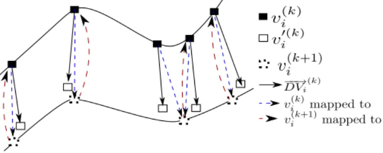
Figure 3: Matching process. Mesh Mkwith vertices v(k)
i is first registered to
mesh Mk+1with vertices v(k+1)
i , inducing new vertices v
′(k)
i . Displacement
vec-tors DVi(k)are defined thanks to this registration. Finally, mappings from Mk
to Mk+1and from Mk+1to Mkare computed.
3.2.1. Mesh registration
The matching stage of our approach aims at establishing a dense cross parametrization between pairs of successive meshes of the sequence. Among the many available algorithms for this task, we chose to favor generality by casting the problem as the registration of two sets of points and normals. This means that we exclusively use geometric cues to align the two meshes, even when photometric information is available like in the case of meshes reconstructed from multi-camera systems. Thus, our approach also handles the case of software generated mesh se-quences.
We implemented the method of Cagniart et al. [7] that itera-tively deforms the mesh Mkto fit the mesh Mk+1. This approach
decouples the dimensionality of the deformation from the com-plexity of the input geometry by arbitrarily dividing the surface into elements called patches. Each of these patches is associ-ated to a rigid frame that encodes for a local deformation with respect to the reference pose Mk. The optimization procedure
is inspired by ICP as it iteratively re-estimates point correspon-dences between the deformed mesh and the target point set and then minimizes the distance between the two point sets while penalizing non rigid deformations of a patch with respect to its neighbors. Running this algorithm in a coarse-to-fine manner by varying the radii of the patches has proven in our experi-ments to robustly converge, and to be faster than using a single patch-subdivision level.
3.2.2. Mappings and displacement vectors computation
By using the previous stage, we get the registered mesh M′k of the mesh Mk on mesh Mk+1. The displacement vector of each vertex v(k)i in Mk,0 6 i < nv(Mk) is then defined as:
DVi(k)= v′(k)i −v(k)i ,
with v′(k)i the corresponding vertex in M′k. To create a
map-ping from Mkto Mk+1, the closest vertex in Mk+1is found for each vertex v′(k)i in M′k using Euclidean distance. A mapping
from Mk+1 to Mkis also created by finding for each vertex in Mk+1 the closest vertex in M′k. Both mappings are necessary
for the subsequent stage of our algorithm (see Sections 3.3.1 and 3.3.4). Note that mesh Mk+1 is not registered to mesh Mk
to compute the second mapping. Apart from saving computa-tion time, this reduces inconsistencies between the two map-pings: in most (though not all) cases, if v(k)i is mapped to v(k+1)i , then v(k+1)i is mapped to v(k)i . Also, note that these mappings are defined on the vertex sets. Hence, topology changes are not handled here. This is done in the next stage.
Using Euclidean distance instead of geodesic one may lead to occasional mismatchs. However, error hardly accumulates thanks to our handling of topology changes, see Section 3.3.4.
3.3. Mesh segmentation
In this part the goal is to create a segmentation Σkof the mesh Mkinto rigidly moving components. The displacement vectors
over a small time window computed during the previous stage are used, as well as (if k , 1) the segmentation Σk−1 of Mk−1 mapped to Mk thanks to the bi-directional mapping between meshes Mk−1and Mk. This provides an initial segmentation es-timate Σk
est of Mk. For k = 1, the initial estimate is the trivial
segmentation of M1 into a single segment, containing all ver-tices v(1)i of M1.
We proceed in four successive steps. First, the motion of each vertex v(k)i of Mkis estimated using the displacements
vec-tors (Section 3.3.1). Then, unless a coherent segmentation is required, neighboring segments in Σk
estthat present similar
mo-tions are merged (Section 3.3.2). Then a spectral clustering ap-proach is used to refine the segmentation. This yields the seg-mentation Σkof the vertices of Mk(Section 3.3.3). Finally, Σk
is mapped onto Mk+1
, to create the initial estimate Σk+1 est of Σk+
1 (Section 3.3.4).
Our segmentation algorithm produces, by construction, con-nected segments since the atomic operations over segments are: merging neighboring segments (see Section 3.3.2) and splitting a segment into connected sub-segments (see Section 3.3.3).
3.3.1. Motion estimate
To estimate the motion of each vertex v(k)i of Mk, the
rigid transformation which maps v(k)i together with its one-ring neighborhood Ng(v(k)i ) onto M′kis computed, using Horn’s method [16]. This method estimates a 4 × 4 matrix represent-ing the best rigid transformation between 2 point clouds. A transformation matrix Ti(k) is therefore associated to each ver-tex v(k)i . With such a method however, computed estimates are noise sensitive, and slow motion is hardly detected. This is due to the fact that only the two meshes Mkand M′k are used. In
order to improve robustness of motion estimates, we propose to work on a time window. Motion is estimated from Mlto M′k
,
Mlbeing the mesh where the segment has been created, either by splitting (see Section 3.3.3) or merging (see Section 3.3.2) of previous segments, or at the beginning of the process (l = 1).
lmay be different for different vertices v(k)i of Mk. Vertex v(l)j of
Mlfrom which motion is estimated is defined using the previ-ously computed bi-directional mapping. This method allows to detect slow motion (see Figure 4), and is less sensitive to noise and matching errors. Notice that different parts of the mesh may move with different speeds, this is not a problem as long as they belong to different segments, since the size of the time window is segment-dependent.
Figure 4: Three successive meshes Mk(blue), Mk+1(purple) and Mk+2(red). Black dots correspond to vertices with null motion. Motion (black arrows) between Mkand Mk+1, then between Mk+1and Mk+2, is too slow to be detected
by our subsequent stage (Section 3.3.3). Using a larger time window [k, k + 2] allows to detect this motion.
3.3.2. Merging
In the case of a variable segmentation, neighboring segments with similar motions before are merged at each time step refin-ing the current segmentation. To this aim, the rigid transforma-tion T(k)(S ) of any segment S is estimated over all its vertices, using Horn’s method [16], as the rigid transformation Ti(k) of any vertex v(k)i and its 1-ring neighborhood has been estimated. A greedy algorithm is then used:
• starting with the segment S with the minimal residual er-ror, this segment is merged with all neighboring segments
S′ such that klog(T(k)(S )−1T(k)(S′))k < T
merge. Tmerge
is a user-defined threshold distance between the transfor-mations of neighboring segments (see Section 3.1). The
choice of this logarithm-based distance between transfor-mations is explained in next section;
• the residual error for the new segment S ∪S S′is com-puted;
• we iterate, merging the next segment with the minimal residual error with its neighbors.
We stop when no merging is possible anymore. Note that this algorithm allows to handle topology changes such as merging of connected components.
The residual error for a segment S corresponds to the mean distance, for all points v(k)i of this segment, between the point
v(k+1)i and the location of v(k)i after the computed rigid transfor-mation T(k)(S ) is applied: ResidualError(S ) = X v(k)i ∈S kv(k+1)i −T(k)(S ) ∗ v(k)i k card(S ) (1)
In our implementation, the choice of the threshold value
Tmergeis left to the user. According to our experiments, it needs
a few trials to find a suitable value. Choosing a high value merges most of the segments, while choosing a low value gen-erates many clusters. The following values have been chosen for the displayed results in Sections 4 and 5: 0.03 for the
Bal-loonand the Horse sequences (Figures 9 and 11), 0.05 for the
Dancersequence (Figure 9) and 0.2 for the Cat sequence (Fig-ure 13).
During the next step the current segmentation is refined. In order to prevent successive and useless merge and split of the same segments, we actually apply motion-based spectral clus-tering on detected pairs of segments to be merged before merg-ing them. If the clustermerg-ing results in some pairs splittmerg-ing, then these pairs are not merged.
3.3.3. Motion-based spectral clustering
Spectral clustering is a popular and effective technique to robustly partition a graph according to some criterion [28]. It has been successfully applied to static meshes (see e.g. [26, 27, 34, 36]), using the mesh vertices as the graph nodes and the mesh edges as the graph edges. The graph should be weighted with respect to the partition criterion. More precisely, edge weights represent similarity between their endpoints. In our case, these weights are related to the motion of neighboring vertices. This is in contrast to [1] where Euclidean distances between vertices are considered. In fact Euclidean distances can be preserved by non rigud transformation. Related to our approach is Brox and Malik’s motion-based segmentation algo-rithm for videos [6].
Edge weights. To compute the weights W(k)of the graph edges, the following expression is used [30]:
w(k)i, j = 1 klog(Ti(k)−1T(k)j )k2 if i , j, 0 if i = j. (2)
As demonstrated in [30], this distance is mathematically founded since it corresponds to distances on the special Eu-clidean group of rigid transformations S E(3).
Spectral clustering algorithm. Using the weighted adjacency matrix W(k), the normalized Laplacian matrix L(k)
rwis built as
fol-lows. Then the well-known Shi and Malik’s normalized spec-tral clustering algorithm [35] is used to segment the graph.
D(k)ii = X
j∈Ng(v(k)i )
wi j(k). (3)
L(k)= D(k)−W(k). (4)
L(k)rw= D(k)−1L(k)= I(k)−D(k)−1W(k). (5) Shi and Malik compute the first K eigenvectors u1, . . . ,uK of L(k)rw and store them as columns of a matrix U. The rows yi,i = 1 . . . n, of U are then clustered using the classical K-means algorithm. Clusters for the input graph correspond to clusters of the rows yi: points i such that yibelong to the same
cluster are said to belong to the same segment of the graph. This method assumes the number K of clusters to be known.
K is computed using the classical eigengap method: let λ1, λ2, . . . , λK, . . . be the eigenvalues of L(k)rwordered by
increas-ing value, the smaller K such that λK− λK−1>eigengapis cho-sen. In our implementation, the eigengap value’s choice is left to the user. In our experiments, a few trials (less than 5) were necessary to set this parameter. Two parameters are also used to prevent the creation of small segments in non-rigid areas (see Section 3.1): a minimum segment size and a maximum subdi-vision of a segment. According to our experiments, results are not very sensitive to the choice of these three parameters; the same values have been used for most of our experiments (see Section 4).
3.3.4. Mapping to Mk+1
The segmentation is computed at each time step on the cur-rent mesh Mk. Labels are then mapped onto the mesh Mk+1 using the bi-directional mapping defined in Section 3.2.2. Seg-ments are first transferred using the mapping from Mkto Mk+1. Then for all unmatched vertices in Mk+1, the mapping from Mk+1 to Mk is used. Segments which are mapped on
differ-ent connected compondiffer-ents are split, see Figure 5. This allows us to naturally handle topology changes. This segmentation of
Mk+1serves as an initial estimate for the computation of Σk+1. Note that segment splitting and merging allows to robustly handle mismatching, see Figure 6. In case a vertex v(k)i is wrongly matched to a vertex v(k+1)j , the corresponding segment is split in two. The new segment containing v(k+1)j is then likely to be merged with a neighboring segment with similar motion.
3.4. Coherent segmentation
The algorithm can be modified to generate a coherent seg-mentation instead of a variable segseg-mentation. This coherent segmentation clusters neighboring vertices that share similar rigid motion over the whole sequence. In other words, as long
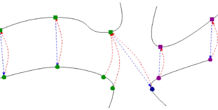
Figure 5: Splitting process. Blue and red arrows indicate the bi-directional mapping. The current segment (black squares) is split in two (green and ma-genta dots, respectively), since the three leftmost vertices and the two rightmost vertices are mapped to two different connected components.
Figure 6: Segment splitting and merging allows to robustly handle mismatch-ing. In case a vertex (rightmost green square) of Mkis mismatched to a vertex
(dark blue dot) of Mk+1, a new segment is created. This segment is then likely
to be merged with the neighboring segment (magenta dots), since they present similar motions.
as their motion differs over at least one small time window, two neighboring vertices do not belong to the same segment.
Creating a coherent segmentation is then straightforward. We only need:
• not to merge segments (step described in Section 3.3.2 is not applied);
• to map the segmentation Σf of the last mesh Mf back to
the whole sequence.
To this purpose, the bi-directional mapping described in Sec-tion 3.2.2 is simply applied in reverse order, from Mf to M1. For each pair of successive meshes (Mk,Mk+1) we first use the mapping from Mk+1 to Mk, then for all vertices of Mkwhich
are not assigned to a segment, the mapping from Mkto Mk+1is used.
4. Results
In this section we show and discuss visual results of our al-gorithm. A quantitative evaluation of these results is discussed in the next section. We first examine matching results, then seg-mentation results on difficult cases (temporally incoherent mesh sequences with topological changes, acquired from real data). We also show that our results on temporally coherent mesh se-quences are visually similar to state-of-the-art approaches.
4.1. Matching results
The vertex matching computation is an important step since our segmentation algorithm relies on it (see Figure 2). Fig-ure 7 shows the result of vertex matching between two succes-sive meshes of a TIMS. Computation time is about 30 seconds for two meshes with approximately 7000 vertices each. This outperforms the matching method proposed in [2] which takes about 13 minutes to complete computation with the same data, for a similar result. Note that outliers in the matching are not explicitly taken into account in the segmentation, however their influence is limited by the threshold on the minimum segment size (see Section 3.1) that tends to force them to merge with neighboring segments.
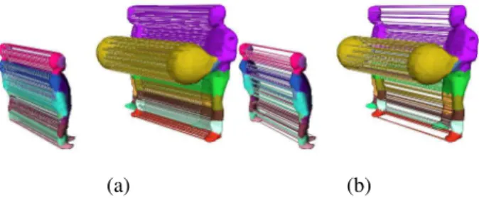
(a) (b)
Figure 7: Result of vertex matching on real data captured from video cameras. (a) Full display. (b) Partial display.
Figure 8 shows a matching result between two consecutive frames of a sequence where the vertex density differs drasti-cally. Even if vertex-to-vertex matching is less accurate than
vertex-to-face matching (that is to say, matching every vertex of Mkto the closest point of Mk+1, which can lie on an edge or inside a face), in our experiments it has proved to be sufficient for our purpose. Meanwhile, its computation is much faster.
Figure 8: Result of vertex matching between two consecutive frames of a se-quence with varying vertex density.
4.2. Segmentations of TIMS with topology changes
Figure 9 shows variable segmentations computed on two
Bal-loonand Dancer sequences. Figure 10 shows coherent segmen-tations computed on the Balloon sequence. By construction, coherent segmentations contain more segments than variable segmentations since no merging operation occurs. Parameters for both variable and coherent segmentations of the Balloon se-quence have the same values, except for the eigengap threshold that is slightly lower in the variable segmentation case (0.40 vs. 0.48 for result shown on Figure 10 (a)). According to our ex-periments, suitable parameter values for a given sequence are found in a few trials. The computation time of one mesh seg-mentation of the Dancer sequence is approximately 3 minutes with a (not optimized) Matlab implementation. Additional re-sults appear in the accompanying video. Our algorithm does not require the whole sequence in memory at a given time step k, but only previous meshes which share at least one segment with the current segmentation, in addition to the next mesh (namely, meshes from Mlto Mk+1, see Section 3.3.1). Thus, it can handle long sequences with a high number of vertices, such as the
Bal-loonsequence which contains 300 meshes with approximately 15,000 vertices each.
Timings are given in the following table. The algorithm was implemented using Matlab on a laptop with a one-core 2.13 GHz processor.
Segmentation Total computation time
Fig. 9 (a–c) 43 min 14
Fig. 9 (d–g) 76 min 48
Fig. 12 (a) 29 min 07
Fig. 12 (b) 25 min 57
Fig. 13 (a) 3 min 46
4.3. Segmentation of TCMS
Although our approach is designed for general cases, it can also handle TCMS and obtains visually similar results to previ-ous TCMS-dedicated methods, as shown in Figure 11.
Figure 12 illustrates the influence of the eigengap threshold: the higher the eigengap value, the coarser the segmentation.
(a) (b) (c)
(d) (e) (f) (g)
Figure 9: (a,b,c) Variable segmentation generated by our algorithm on the Dancer sequence [38]. First meshes are decomposed into 6 segments, then the right arm and right hand segments merge since they move the same way. Finally, this segment is split again. Note that topology changes can be handled (in the last meshes, the left arm is connected to the body). (d,e,f,g): Variable segmentation of a sequence with 15,000 vertices per mesh and topology changes. The balloon is over-segmented because its motion is highly non rigid.
(a) (b)
Figure 10: Coherent segmentation results on the Balloon sequence, obtained with two different eigengap values: (a) 0.48, (b) 0.8. Segments cluster neigh-boring vertices that share the same motion over the whole sequence.
(a) (b)
(c) (d)
Figure 11: Segmentation results on a TCMS. (a) [23]. (b) [1]. (c) [2]. (d) Our method.
(a) (b)
Figure 12: Segmentation of the Horse sequence [39] with two different eigen-gap values. (a) eigeneigen-gap = 0.7. (b) eigeneigen-gap = 0.5.
5. Evaluation
A quantitative and objective comparison of segmentation methods is an ill-posed problem since there is no common defi-nition of what an optimal segmentation should be in the general case. Segmentation evaluation has been recently addressed in the static case using ground truth (i.e. segmentations defined by humans) [5, 9]. In the mesh sequence case, none of the previ-ously cited articles in Section 2 proposes an evaluation of the obtained segmentations. We thus propose the following frame-work to evaluate a mesh sequence segmentation method.
5.1. Optimal segmentation
The optimal segmentation of a mesh sequence, be it a TCMS or a TIMS, into rigid components can be guessed when the motion and/or the kinematic structure is known. This is, for instance, the case with skeleton-based mesh animations, as created in the computer graphics industry. In this case, each mesh vertex of the sequence is attached to at least one (usually, no more than 4) joints of the animation skeleton, with given weights called skinning weights. These joints are organized in a hierarchy, which is represented by the “bones” of the skeleton that are, therefore, directed. For our evaluation, we attach each vertex to only one joint among the related joints, the furthest in the hierarchy from the root joint. If this joint is not unique, the one with the greatest skinning weight is kept. Each joint has its own motion, but several joints can move together in a rigid manner. For a given mesh, cluster joints of the animation skeleton can therefore be clustered into joint sets, each joint set representing a different motion. We now define as an optimal
segmentthe set of vertices related to joints in the same joint set. Since the motion of each joint is known, we exactly know, for each mesh of the animation, what are the optimal segments.
This definition can be applied in the general case of TIMS, provided that each vertex of each mesh can be attached to a joint. However, we only tested it in the more convenient case of a TCMS.
5.2. Error metrics
We propose the following three metrics in order to evaluate a given segmentation with respect to the previously defined opti-mal segmentation:
• Assignment Error(AE): for a given mesh, the ratio of ver-tices which are not assigned to the correct segment. This includes the case of segments which are not created, or which are wrongly created;
• Global Assignment Error(GAE): the mean AE among all
meshes of the sequence;
• Vertex Assignment Confidence(VAC): for a given vertex of a TCMS, the ratio of meshes in which the vertex is as-signed to the correct segment.
AE and GAE give a quantitative evaluation of a mesh segmen-tation and the mesh sequence segmensegmen-tation, respectively, with respect to the optimal segmentation. VAC can help to locate wrongly segmented areas.
Note that more sophisticated evaluation metrics exist to com-pare two static mesh segmentations [9]. We define AE as a sim-ple ratio for sake of simplicity, but other metrics can also be used to define global assignment errors.
5.3. Evaluation results
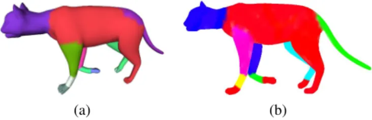
We tested our algorithm on a walking cat skeleton-based an-imation (see Figure 13 and the accompanying video). We get a variable segmentation with a AE up to 17%, in the worst case. Wrongly assigned vertices correspond to the cat skin around joints and to a wrong subdivision in cat paw, i.e. in the less rigid areas.
(a) (b)
Figure 13: Result on a skeleton-based synthetic animation. (a) Computed vari-able segmentation. (b) Optimal varivari-able segmentation, for the same mesh of the sequence.
In the case of coherent segmentations, and if matching is-sues are not taken into account, then the AE is the same for all meshes. Therefore, the GAE is equal to the AE of any mesh. For the cat sequence, the GAE is also 17%. The VAC can be 0% or 100%, and is only relevant as a relative criterion to compare vertices and find ill-segmented areas. On the cat sequence ver-tices in rigid areas (paws, tail, body) are often always assigned to the correct segment; their confidence is equal to 1. In con-trast, some vertices around joints can be assigned to the same neighboring segment in all meshes; their confidence drops to 0, see Figure 14. We also computed these metrics for the method described in [2], using the same cat sequence. The GAE reaches 42%, while the VAC can also be 0% or 100%.
6. Conclusion
In this paper we addressed the problem of 3D mesh sequence segmentation into rigidly moving components. We have pro-posed a classification of mesh sequence segmentations, together
Figure 14: Vertex Assignment Confidence results. Vertices for which VAC is 0 are colored in red, while vertices with confidence equal to 1 are in black.
with a segmentation method that takes as input a mesh se-quence, even when no explicit temporal coherence is available, and possibly with topology changes. This method produces ei-ther a coherent or a variable segmentation into rigid compo-nents depending on the user’s choice. It uses a few parameters which can be set in a few trials, according to our experiments. We have also proposed a framework for quantitative evaluations of rigid segmentation methods.
6.1. Current limitations
We are currently aware of three limitations in the proposed algorithm:
• our method clearly depends on the quality of the matching process. Important errors in matching computation may lead to wrong results;
• segmentation can slightly drift: this is due to the fact that only 2 meshes are considered when matching;
• segments which are wrongly subdivided are transferred to the following meshes, meaning that errors on an early mesh in the sequence can affect the whole segmentation. Such errors are generally due to errors in the matching process. This issue is less critical on variable segmenta-tions than on coherent segmentasegmenta-tions, since segments are merged later.
Figure 15 shows an example of these limitations. In this ex-ample, the entire left front leg of the horse at frame k was in-tentionally mismatched to the right front leg at frame k + 1, and vice-versa. Resulting erroneous segmentation at frame k + 1 is then propagated to the following frames, since no merging with the neighboring segment occurs. Fortunately, this problem sel-dom happens. As shown in our quantitative evaluations, using the matching process described in Section 3.2, vertices that are wrongly assigned to a segment are located near articulations. Vertices in rigid regions are generally correctly clustered.
Despite these limitations, our method has shown as good re-sults as current state-of-the-art methods on temporally coherent mesh sequences (see Figure 11), although it has been designed for the more difficult case of mesh sequences without temporal coherence.
(a) (b) (c)
Figure 15: Matching error and resulting coherent segmentation. (a,b) Two con-secutive frames of the Horse sequence. (c) Matching between these two frames.
6.2. Future work
Our method can be improved in various ways. As explained above, it would be interesting to improve the vertex assign-ments around articulations. Adding prior knowledge about the geometry of desired segments (e.g. cylindrical shape, or sym-metry information) would be helpful to enhance the robustness of the method. It would also be useful to reduce the number of parameters. Our algorithm handles topology changes, but our solution is not semantically satisfactory in case a new con-nected component (e.g., the shade of the balloon in the Balloon sequence) appears, since it is first attached to an existing seg-ment before being split from it.
We hope our evaluation metrics would be helpful for further work in the domain. However, a more in-depth study of the three proposed criteria need to be performed to assess their use-fulness. Finally, a user validation can also help to quantify seg-mentations produced by our algorithm.
Acknowledgments
The Balloon sequence is courtesy of Inria Grenoble [18]. The
Dancersequence is courtesy of University of Surrey [38]. The
Horsesequence is courtesy of M.I.T. [39]. The Cat sequence is courtesy of Inria Grenoble [4]. This work has been partially funded by the french National Reseach Agency (ANR) through the MADRAS 07-MDCO-015) and MORPHO (ANR-10-BLAN-0206) projects.
References
[1] de Aguiar, E., Theobalt, C., Thrun, S., Seidel, H., 2008. Automatic con-version of mesh animations into skeleton-based animations. Computer Graphics Forum (Eurographics proceedings) 27.
[2] Arcila, R., Buddha, K., H´etroy, F., Denis, F., Dupont, F., 2010. A frame-work for motion-based mesh sequence segmentation, in: Proceedings of the International Conference on Computer Graphics, Visualization and Computer Vision (WSCG).
[3] Attene, M., Falcidieno, B., Spagnuolo, M., 2006. Hierarchical mesh seg-mentation based on fitting primitives. The Visual Computer 22. [4] Aujay, G., H´etroy, F., Lazarus, F., Depraz, C., 2007. Harmonic skeleton
for realistic character animation, in: Proceedings of the Symposium on Computer Animation (SCA).
[5] Benhabiles, H., Vandeborre, J., Lavou´e, G., Daoudi, M., 2009. A framework for the objective evaluation of segmentation algorithms us-ing a ground-truth of human segmented 3D-models, in: Proceedus-ings of the IEEE International Conference on Shape Modeling and Applications (SMI).
[6] Brox, T., Malik, J., 2010. Object segmentation by long term analysis of point trajectories, in: Proceedings of the European Conference on Com-puter Vision (ECCV).
[7] Cagniart, C., Boyer, E., Ilic, S., 2010. Iterative deformable surface track-ing in multi-view setups, in: Proceedtrack-ings of the International Symposium on 3D Data Processing, Visualization and Transmission (3DPVT). [8] Cashman, T., Hormann, K., 2012. A continuous, editable representation
for deforming mesh sequences with separate signals for time, pose and shape. Computer Graphics Forum (Eurographics proceedings) 31. [9] Chen, X., Golovinskiy, A., Funkhouser, T., 2009. A benchmark for 3d
mesh segmentation. ACM Transactions on Graphics (SIGGRAPH pro-ceedings) 28.
[10] Cutzu, F., 2000. Computing 3d object parts from similarities among ob-ject views, in: Proceedings of the IEEE Conference on Computer Vision and Pattern Recognition (CVPR).
[11] Cuzzolin, F., Mateus, D., Knossow, D., Boyer, E., Horaud, R., 2008. Co-herent laplacian 3-d protrusion segmentation, in: Proceedings of the IEEE Conference on Computer Vision and Pattern Recognition (CVPR). [12] Fang, Y., Sun, M., Kim, M., Ramani, K., 2011. Heat mapping: a robust
approach toward perceptually consistent mesh segmentation, in: Proceed-ings of the IEEE Conference on Computer Vision and Pattern Recognition (CVPR).
[13] Franco, J., Boyer, E., 2011. Learning temporally consistent rigidities, in: Proceedings of the IEEE Conference on Computer Vision and Pattern Recognition (CVPR).
[14] de Goes, F., Goldenstein, S., Velho, L., 2008. A hierarchical segmen-tation of articulated bodies. Computer Graphics Forum (Symposium on Geometry Processing proceedings) 27.
[15] Goldenthal, R., Harmon, D., Fattal, R., Bercovier, M., Grinspun, E., 2007. Efficient simulation of inextensible cloth. ACM Transactions on Graphics (SIGGRAPH proceedings) 26.
[16] Horn, B., 1987. Closed-form solution of absolute orientation using unit quaternions. J. Opt. Soc. Am. A 4.
[17] Huang, Q., Wicke, M., Adams, B., Guibas, L., 2009. Shape decompo-sition using modal analysis. Computer Graphics Forum (Eurographics proceedings) 28.
[18] Inria, . Balloon sequence.http://4drepository.inrialpes.fr/. [19] Kalafatlar, E., Yemez, Y., 2010. 3d articulated shape segmentation using
motion information, in: Proceedings of the International Conference on Pattern Recognition (ICPR).
[20] Kalogerakis, E., Hertzmann, A., Singh, K., 2010. Learning 3d mesh seg-mentation and labeling. ACM Transactions on Graphics (SIGGRAPH proceedings) 29.
[21] Kircher, S., Garland, M., 2006. Editing arbitrarily deforming surface animations. ACM Transactions on Graphics (SIGGRAPH proceedings) 25.
[22] Lee, N., T.Yamasaki, Aizawa, K., 2008. Hierarchical mesh decomposi-tion and modecomposi-tion tracking for time-varying-meshes, in: Proceedings of the IEEE International Conference on Multimedia and Expo (ICME). [23] Lee, T.Y., Wang, Y.S., Chen, T.G., 2006. Segmenting a deforming mesh
into near-rigid components. The Visual Computer 22.
[24] Lengyel, J., 1999. Compression of time-dependent geometry, in: Pro-ceedings of the Symposium on Interactive 3D graphics (I3D).
[25] Lewis, J., Cordner, M., Fong, N., 2000. Pose-space deformation: a uni-fied approach to shape interpolation and skeleton-driven deformation, in: Proceedings of SIGGRAPH.
[26] Liu, R., Zhang, H., 2004. Segmentation of 3d meshes through spectral clustering, in: Proceedings of Pacific Graphics.
[27] Liu, R., Zhang, H., 2007. Mesh segmentation via spectral embedding and contour analysis. Computer Graphics Forum (Eurographics proceedings) 26.
[28] von Luxburg, U., 2007. A tutorial on spectral clustering. Statistics and Computing 17.
[29] Marras, S., Bronstein, M.M., Hormann, K., Scateni, R., Scopigno, R., 2012. Motion-based mesh segmentation using augmented silhouettes. Graphical Models .
[30] Murray, R., Sastry, S., Zexiang, L., 1994. A Mathematical Introduction to Robotic Manipulation. CRC Press, Inc.
[31] Reuter, M., 2010. Hierarchical shape segmentation and registration via topological features of laplace-beltrami eigenfunctions. International Journal of Computer Vision 89.
[32] Rosman, G., Bronstein, M.M., Bronstein, A.M., Wolf, A., Kimmel, R., 2011. Group-valued regularization framework for motion segmentation of dynamic non-rigid shapes, in: Scale Space and Variational Methods in Computer Vision.
[33] Shamir, A., 2008. A survey on mesh segmentation techniques. Computer Graphics Forum 27.
[34] Sharma, A., von Lavante, E., Horaud, R., 2010. Learning shape segmen-tation using constrained spectral clustering and probabilistic label trans-fer, in: Proceedings of the European Conference on Computer Vision (ECCV).
[35] Shi, J., Malik, J., 2000. Normalized cuts and image segmentation. IEEE Transactions on Pattern Analysis and Machine Intelligence (PAMI) 22. [36] Sidi, O., van Kaick, O., Kleiman, Y., Zhang, H., Cohen-Or, D., 2011.
Un-supervised co-segmentation of a set of shapes via descriptor-space spec-tral clustering. ACM Transactions on Graphics (SIGGRAPH Asia pro-ceedings) 30.
[37] Skraba, P., Ovsjanikov, M., Chazal, F., Guibas, L., 2010. Persistence-based segmentation of deformable shapes, in: CVPR Workshop on Non-Rigid Shape Analysis and Deformable Image Alignment.
[38] Starck, J., Hilton, A., 2007. Surface capture for performance-based ani-mation. IEEE Computer Graphics and Applications .
[39] Sumner, R., Popovi´c, J., 2004. Deformation transfer for triangle meshes. ACM Transactions on Graphics (SIGGRAPH proceedings) 23. [40] Tung, T., Matsuyama, T., 2009. Topology dictionary with markov model
for 3d video content-based skimming and description, in: Proceedings of the IEEE Conference on Computer Vision and Pattern Recognition (CVPR).
[41] Tung, T., Matsuyama, T., 2010. 3d video performance segmentation, in: Proceedings of the IEEE International Conference on Image Processing (ICIP).
[42] Varanasi, K., Boyer, E., 2010. Temporally coherent segmentation of 3d reconstructions, in: Proceedings of the International Symposium on 3D Data Processing, Visualization and Transmission (3DPVT).
[43] Vlasic, D., Baran, I., Matusik, W., Popovi´c, J., 2008. Articulated mesh animation from multi-view silhouettes. ACM Transactions on Graphics (SIGGRAPH proceedings) 27.
[44] Wuhrer, S., Brunton, A., 2010. Segmenting animated objects into near-rigid components. The Visual Computer .
[45] Yamasaki, T., Aizawa, K., 2007. Motion segmentation and retrieval for 3d video based on modified shape distribution. EURASIP Journal on Applied Signal Processing .


![Figure 9: (a,b,c) Variable segmentation generated by our algorithm on the Dancer sequence [38]](https://thumb-eu.123doks.com/thumbv2/123doknet/14460537.520366/9.892.90.817.119.543/figure-b-variable-segmentation-generated-algorithm-dancer-sequence.webp)