Acoustic signal estimation using multiple blind observations

Acoustic Signal Estimation using Multiple Blind

Observations

by

Joonsung Lee

Submitted to the Department of Electrical Engineering and Computer

Science

in partial fulfillment of the requirements for the degree of

Master of Science

at the

MASSACHUSETTS INSTITUTE OF TECHNOLOGY

January 2006

( Massachusetts Institute of Technology 2006. All rights

7/.X Hi-K '

-lUblI

...

Department of Electrical Engineering and Computer Science

Certified

by ...

...

Charles E. Rohrs

Research Scientist

Accepted by

Thesis Supervisor

Arthur C. Smith

Chairman, Department Committee on Graduate Students

OF TECHNOLOGY

JUL 10 2006

LIBRARIES

ARCHNES

--Acoustic Signal Estimation using Multiple Blind

Observations

by

Joonsung Lee

Submitted to the Department of Electrical Engineering and Computer Science

on January 31, 2006, in partial fulfillment of the requirements for the degree of

Master of Science

Abstract

This thesis proposes two algorithms for recovering an acoustic signal from multiple blind measurements made by sensors (microphones) over an acoustic channel. Unlike other algorithms that use a posteriori probabilistic models to fuse the data in this problem, the proposed algorithms use results obtained in the context of data com-munication theory. This constitutes a new approach to this sensor fusion problem. The proposed algorithms determine inverse channel filters with a predestined support (number of taps).

The Coordinated Recovery of Signals From Sensors (CROSS) algorithm is an in-direct method, which uses an estimate of the acoustic channel. Using the estimated channel coefficients from a Least-Squares (LS) channel estimation method, we pro-pose an initialization process (zero-forcing estimate) and an iteration process (MMSE estimate) to produce optimal inverse filters accounting for the room characteristics, additive noise and errors in the estimation of the parameters of the room character-istics. Using a measured room channel, we analyze the performance of the algorithm through simulations and compare its performance with the theoretical performance. Also, in this thesis, the notion of channel diversity is generalized and the Averaging Row Space Intersection (ARSI) algorithm is proposed. The ARSI algorithm is a direct method, which does not use the channel estimate.

Thesis Supervisor: Charles E. Rohrs Title: Research Scientist

Acknowledgments

First of all, I'd like to express my sincere gratitude to God and His son, my Lord Jesus Christ, who have guided me to this place, made me to meet my great supervisor, Charlie, and gave me strength and peace all the time.

To my research supervisor Charlie. You know my strengths and weaknesses. You have guided me, encouraged me, and especially you believed me that I could do this. To my academic advisor Al Oppenheim. Not only for my research, but also for my life at MIT and US, you took care of me and helped me. Your freshman seminar

helped me a lot to get to know MIT. Your comments during the group meeting

enlarged my scope of thinking.

I also want to thank all the DSPG: Zahi, Alaa, Petros, Sourav, Ross, Melanie,

Tom, Joe, Maya, Dennis, Matt, and Eric. I want to thank especially Ross who

collected data which I used for experiments and simulations, read my thesis over and over, and helped me write without missing any ideas. I want to thank Zahi for making me win almost all the squash games and your endless help.

Let me acknowledge the generous financial support of the Korea Foundation for

Advanced Studies (KFAS). I'll do my best to contribute to the society. Lastly, thank you, dad, mom, and my brothers Daesung and Hyosung. Thank you all.

Contents

1 Introduction

1.1 Blind Signal Estimation over Single-Input Multi-Output Channel

1.1.1 Signal Model: Single-Input Multi-Output (SIMO) Model

1.2 Problem Statement ... 1.3 Constraints ...

1.3.1 Linear Complexity of the Input Signal ... 1.3.2 Diversity Constraint of the Channel ...

1.4 Two General Approaches of Estimating the Input Signal ... 1.4.1 Indirect Method ...

1.4.2 Direct Method ... 1.5 Outline of the Thesis ... 1.6 Contributions of this Thesis ...

2 Background

2.1 Signal Model in a Matrix Form ... 2.1.1 Notation.

2.1.2 Equivalent Signal Models ...

2.2 Order Estimation ...

2.2.1 Naive Approach: Noiseless Case ...

2.2.2 Effective Channel Order Estimation .... 2.3 Least Squares Blind Channel Estimation Method

2.3.1 Notation. 2.3.2 Algorithm ... 13 .. 13 . . 14 . . 15 . . 16 . . 16 . . 17 . . 18 . . 19 . . 20 . . 21 . . 23 25 . . . .. . . . .25

... . .25

... . .28

... . .29

... . .30

... . .32

... . .32

... . .32

2.3.3 Performance. ...

2.4 Singular Value Decomposition (SVD) ... 3 Diversity of the Channel

3.1 Properties ...

3.2 Definition of Diversity ...

3.3 Diversity with Finite Length Signals . . .

3.4 Examples: Small Diversity ...

3.4.1 Common Zeros.

3.4.2 Filters with the Same Stop Band 3.4.3 Small leading or tailing taps .... 3.5 Effective Channel Order Revisited ...

3.6 Diversity over a Constrained Vector Space

4 Linear MMSE Signal Estimate of the Input given t

of the Channel: The CROSS Algorithm

4.1 Mean Square Error of the Input Signal Estimate . . . 4.2 Initializing The CROSS algorithm ...

4.3 IIR Estimate.

4.3.1 Error of the Fourier Domain Representation

4.3.2 Minimizing 2 in terms of G ...

4.3.3 Minimizing Total Error ... 4.3.4 Summary: IIR MMSE Estimate ...

4.4 The CROSS Algorithm - Producing an Optimal Input FIR Filters ...

4.4.1 Toeplitz Matrix Representation of the Sum of 4

4.4.2 Error in a Matrix Form ... 4.4.3 Notation.

4.4.4 Minimizing 2 + 3 in terms of g ...

4.4.5 Minimizing the Total Error .

4.4.6 Initialization: Unbiased Estimate ...

;he LS Estimate . . . . . . . .. . . . .. . . . . .. . . . . . . . 47 47 49 50 51 51 52 53 Estimate Using Convolutions . .. . . .. . . . . . . .. . . . . . . . . . . . . . . .. .. . . 54 55 55 57 59 61 61 33 34 35 35 36 37 39 39 40 43 43 44

...

...

...

...

...

...

...

...

...

4.4.7 Procedure of the CROSS Algorithm ...

5 Analysis

5.1 Simulation

...

...

5.1.1 Typical Room Channels ...

5.1.2 Artificially Generated Measured Signals ... 5.2 Least Squares Channel Estimation Method ... 5.3 The CROSS Algorithm: Inverse Channel Filters ... 5.4 Iteration ...

5.5 Remarks ...

6 Averaging Row Space Intersection

6.1 Isomorphic Relations between Input Row S

6.2 Naive Approach: Noiseless Case ... 6.3 Previous Works: Row Space Intersection

6.4 FIR Estimate.

6.4.1 Vector Spaces to be Intersected . . 6.4.2 Estimate of the Vector Space . . .

6.4.3 Averaging Row Space Intersection .

6.5 Summary: Algorithm ... 6.5.1 Overall Procedure . ...

pace and Output Row Space

6.5.2 The Estimate of the Input Row Vector Spaces,

6.5.3 MMSE Inverse Channel Filters,

fi,---Vi

,fq 7 Conclusion

A Derivation of the distribution of the Channel Estimate A.1 Notation.

A.2 Asymptotic Distribution of G ... A.3 Asymptotic Distribution of F ...

A.3.1 Distribution of Fw ... A.3.2 Distribution of Fx ... 62 63 63 64 64 66 70 . . . .... . . . 71 . . . .... . . . 73 75 75 76 77

... .

79

... .

79

... .

80

... .

81

... .

85

... .

85

... .

85

A.3.3 Distribution of the Channel Estimate . . . .... 98

A.3.4 Asymptotic Performance. ... . . 98 A.4 Asymptotic Performance in the Case of Zero-Mean White Gaussian

Input Signal ... 99

B Relevance of the Definition of the Diversity 103

B.1 Proof of the Properties . . . ... 103

List of Figures

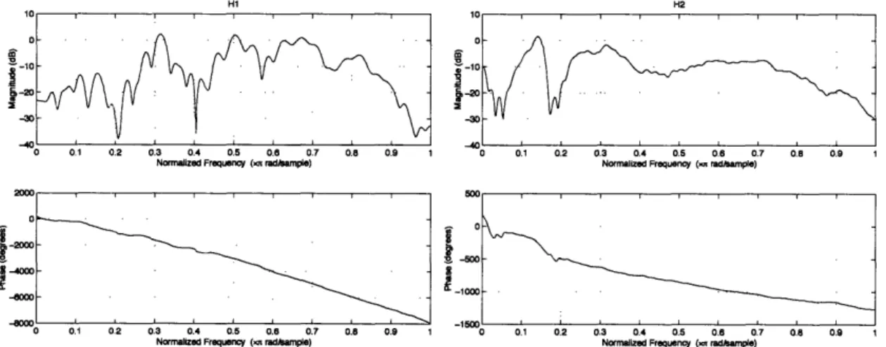
5-1 Two Typical Room Channels(Time Domain) ... 65

5-2 Two Typical Room Channels(Frequency Domain) ... 65

5-3 The Performance of the LS method ... 67

5-4 The Singular Values of TK(h) ... 68

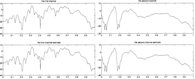
5-5 Actual Channel and Channel Estimate in Frequency Domain ... 69

5-6 The Error in the Frequency Domain ... 69

5-7 The Performance of the CROSS Algorithm with the different number of inverse channel taps ... 71

5-8 The Performance of the CROSS Algorithm: IIR Zero-Forcing vs IIR MMSE ... 71

Chapter 1

Introduction

1.1 Blind Signal Estimation over Single-Input

Multi-Output Channel

It is a common problem to attempt to recover a signal from observations made by two or more sensors. Most approaches to this problem fuse the information from the sensors through an a posteriori probabilistic model. This thesis introduces an entirely different approach to this problem by using results obtained in the context of data communication theory. These previous results are collected under the rubric

of multichannel blind identification or equalization as surveyed in [1].

Consider a case where an independently generated acoustic signal is produced and then captured by a number of microphones. The Coordinated Recovery of Signals

From Sensors (CROSS) algorithm and the Averaging Row Space Intersection (ARSI)

algorithm presented in this thesis apply well if each recorded signal can be well mod-eled by a linear time-invariant (LTI) distortion of the signal with an additive noise component. These algorithms produce estimates of the originating signal and the

characterization of each distorting LTI system. We believe the algorithms may be useful in fusing different modalities of sensors (seismic, radar, etc.) as long as the

LTI model holds and the modalities are excited from a common underlying signal. Finally, these algorithms can be used to remove the LTI distortions of multiple signals

simultaneously as long as there are more sensors than signals. Thus, it is a natural algorithm for adaptive noise cancellation. In this thesis, we discuss only a single

signal. The extension is natural.

In the data communication problem covered in previously published literature, the originating signal is under the control of the system designer and certain properties

of this signal are often assumed. Some of these properties include the use of a finite alphabet [2], whiteness [3], and known second order statistics [4]. However, these

assumptions on the originating signal are inappropriate in the sensor problems we address, and thus we are required to modify and extend the existing theory.

1.1.1 Signal Model: Single-Input Multi-Output (SIMO) Model

We measure the signal of interest using several sensors. We model the channel between the signal and sensors as FIR filters. In this model, measured signals, yl, * *, Yq, can

be written as

yi = hi * x + wi (1.1)

where, indexing of sequences has been supressed, * represents convolution of the

sequence hi[n] with the sequence x[n], and for i = 1, ... , q, the wi[n] are independent wide-sense stationary zero-mean white random processes. The wi are independent

of each other. We assume that we can model the variances of the noises, oi2. By

multiplying by the scalars, , we can normalize the variance of each noise component

into a2. We assume for simplicity of exposition that the variances of wi are all equal

to o2. We assume that the FIR filters, hi, are causal and the minimum delay is zero.

That is,

min{nlhi[n] # 0, for some i = 1, ,q) = 0. (1.2)

Let K be the order of the system, which is the maximum length of time a unit pulse input can effect some output in the system. That is,

With this SIMO FIR model, we can state the goal of blind signal or channel estimation system as the follows:

Goal of Blind Signal or Channel Estimation System

Given only the measurement signals, yl," ,yq, find an implementable algorithm that can be used to estimate the input signal x and/or the channel, hi,... , hq, which minimizes some error criteria.

1.2 Problem Statement

In this thesis, we focus on estimating the input signal. We constrain our estimate of the input signal as a linear estimate, which can be calculated by linear operations on the measured signals. The linear estimate of the input signal, x, can be written as the following:

= fi*y + + fq * yq.

(1.4)

Our goal is to determine the linear estimate of the input signal that minimizes the mean square error between the estimated and the actual signals. We can state

our problem as follows:

Problem Statement:

Given the measured signals, yl, , yq, determine inverse channel filters, fi, fq,

that minimize the mean square error,

E = E[ T2 + 1 ([n] - x[n])2] (1.5)

where the support of the input signal is [T, T2], that is, x[n] = 0 for n < T and

n > T2. In this thesis, we generally assume that the length of the support is sufficiently

performance improves as T2 - T1 increases. We let T1 = 1 and T2 = T to make the notation simple.

1.3 Constraints

Even in the absence of noise, if given only one measurement signal, we cannot

de-termine the input signal without additional prior knowledge. Even with multiple measurements and in the absence of noise, we cannot determine the input signal well if the input signal and the channel do not satisfy certain conditions. Previously pre-sented in [1], the linear complexity and channel diversity constraints are reviewed in this section. If the two constraints are satisfied, the input signal can be determined to within a constant multiplier in the absence of the noise.

For any constant c, the channel, chi,... ,chq, and the input signal, , produce

the same measured signals as the channel, h, * , hq, and the signal x. Only given the measured signals, the input signal cannot be determined better than to within a constant multiplier.

1.3.1 Linear Complexity of the Input Signal

The linear complexity of a deterministic sequence measures the number of memory locations needed to recursively regenerate the sequence using a linear constant co-efficient difference equation. As presented in [1], the linear complexity of the input

signal is defined as the smallest value of m for which there exists {ci} such that

m

x[n] = E cjx[n- j], for all n = N + m, N, 2 (1.6)

j=1

where [N1, N2] is the support of the input signal.

For example, consider the linear complexity of the following signal: x[n] = clsin(aln+

b1) + ... + cMsin(aMn + bM), which is the sum of M different sinusoids. Let xi[n] be

the one particular sinusoid: xi[n] = cisin(ain + bi). Then, x[n] = xl[n] + -. . + xM[n].

xi[n] can be represented as a linear combination of two previous samples: xi[n] =

2cos(ai)xi[n - 1] - xi[n - 2].

To determine the linear complexity of the sum of M sinusoids, let hi[n] = [n]

-2cos(ai)6[n- 1] + i[n - 2]. Then, hi * xi = 0. That is, by putting the sum of sinusoids,

x[n], into the filter hi, we can remove the corresponding sinusoid, xi[n]. Thus, the

output of a cascade connection of all the filters hl, .. , hM with input x[n] is zero.

That is, h

*

The number of taps of the cascaded system, h, * h2 *.. * hM, is 2M + 1; therefore, any sample of x[n] is a linear combination of previous 2M samples of x[n]. The linear complexity of the sum of M different sinusoids is less than or equal to 2M. In fact, we can prove that the linear complexity of the sum of M different sinusoid is 2M by mathematical induction.

This linear complexity is related to the maximum number of independent rows of the following matrix:

x[n] * x[n + k]

x[n-N] ... x[n+ k-N]

For large k, satisfying at least k > N, if the linear complexity is greater than

or equal to the number of rows, the rows of the matrix X are linearly independent

since any row cannot be expressed as a linear combination of the other rows. For

large k, satisfying at least k > N, the rank of the matrix is equal to the number of independent rows. That is, the matrix becomes a full row rank matrix.

We assume that the input signal of our consideration has large linear complexity,

m, such that m >> K in the remainder of this thesis.

1.3.2 Diversity Constraint of the Channel

Assume that the input signal has large linear complexity. The diversity constraint on the channel, h, ... , hq, developed in [1] and restated here is necessary for a solution

to within a constant multiplier. The constraint is that the transfer functions of the

channel in the z-domain (frequency domain) have no common zeros. In other words,

there is no complex number z0 such that Hi(zo), ... , H(zo) are all simultaneously

zero. The proof of necessity and the other details of the diversity constraint are shown

in [1].

In the absence of noise, the combination of the diversity constraint, which is the no common zero constraint, and the linear complexity constraint on the input is

also a sufficient condition for a solution to within a constant multiplier. That is, we

can determine the channel coefficients and input signal to within a constant factor

multiplication as long as the diversity constraint is satisfied. In Chapter 4 and 6,

we show that, in the noiseless case with the diversity and complexity constraints in place, our algorithms can determine the input signal and the channel coefficients to within a scalar multiplication.

However, in the presence of noise, the performance of the input signal estimate depends not only on the channel diversity constraint, but also on the specific values of the channel coefficients. One simple reason is that different channel coefficients

produce different signal to noise ratios (SNR) of the measured signals. Measuring the achievable performance of the input signal estimate from the measured signals in the

presence of noise is ambiguous and has not, to our knowledge, been defined yet. In

Chapter 3, we generalize the idea of the diversity constraint and define a measure of

the diversity in the presence of noise.

1.4 Two General Approaches of Estimating the

In-put Signal

Our problem statement has two sets of unknowns: the input signal and the channel

coefficients. Knowing one of them greatly simplifies the process of estimating the

other. We can estimate the input signal not only through a direct method, but also through an indirect method, which consists of estimating the channel coefficients

and then using the channel coefficients estimates to estimate the input signal. In this section, we introduce the ideas of an indirect method (CROSS Algorithm) and a direct method (ARSI Algorithm) and the differences between our algorithms and algorithms previously developed. We present the details of the CROSS Algorithm in Chapter 4 and the ARSI Algorithm in Chapter 6.

1.4.1 Indirect Method

During the last decade, the problem of blindly estimating the channel coefficients from measured signals has been studied within the context of a data communication problem by many researchers. For the sensor problem we address, we consider three of these methods developed previously: the LS(Least Squares) method [5], the SS(Signal Subspace) method [6], and the LSS(Least Squares Smoothing) method [7]. As shown in [8], if we use only two measurements, the LS and the SS methods produce the same result.

Using the channel estimate, we can estimate the input signal by equalizing the channel. If given the correct channel coefficients, MMSE (minimum mean square

error) equalizers can be determined as is done in [9]. However, we will not have

correct channel information in the presence of noise.

In Chapter 4, we present an algorithm to determine the input signal using the channel estimate from the Least-Squares channel estimation method [5]. Compared to MMSE estimate given in [9] that assumes a correct channel estimate, our algorithm determines inverse channel filters even with a flawed channel estimate. For an ideal situation, where we can use an infinite number of taps for the inverse channel filters, we derive an MMSE Infinite Impulse Response (IIR) equalizer. The IIR equalizer shows a frequency domain view, and the minimum mean square error of the input signal

estimate is derived. For a practical situation, where we can use only a finite number of taps for the inverse channel filters, we present an iterative process for MMSE

Finite Impulse Response (FIR) inverse channel filters. We initialize our process by determining the inverse channel filters' coefficients that minimize one factor of the mean square error. The initialization produces an unbiased or zero-forcing input

signal estimate. We then iterate the process of improving the signal estimate using the knowledge of the distribution of the channel estimate.

1.4.2 Direct Method

As developed in [10] and restated in Section 6.1, isomorphic relations between input

and output row spaces enable us to estimate the vector spaces generated by the rows of Toeplitz matrices of the input signal from the measured signals. We construct Toeplitz matrices of the input signal whose rows are linearly independent except for

one common row. By intersecting the row spaces of the matrices, we can estimate

the common row and, as a by-product, the intersection process itself determines the

coefficients of the inverse channel filters.

Algorithms that use these kinds of row space intersections are developed in [10]

and [11]. The algorithm given in [10] computes the union of the vector spaces that are orthogonal to the row spaces of the input signal matrix estimated by the row spaces of the measured signal matrix. The algorithm then determines the vector that is orthogonal to the union. In the noisy case, it computes the singular vector

corresponding to minimum singular value of the matrix whose rows form a basis for

the union.

The algorithm given in [11] estimates the row spaces of the input signal matrix from the measured signal and then determines the input signal estimate that mini-mizes the sum of distances between the row space of the Toeplitz matrix of the input signal estimate and the row spaces calculated from the measured signal.

The difference between our algorithm and the algorithms given in [10] and [11] is that the algorithms given in [10] and [11] compute the intersection of the row spaces to get an estimate the input signal, while we determine a vector that belongs to

one particular vector space corresponding to the inverse channel filters with a given support, which enables us to determine inverse channel filters with smaller number of

taps than the number of taps required for the other algorithms given in [10] and [11].

Also, under a fixed support of the inverse channel filters, our algorithm uses more row spaces than the other algorithms. Since our algorithm use more vector spaces for

the intersection, the error in the presence of noise is averaged and thus reduced.

1.5 Outline of the Thesis

Chapter 2 presents a review of existing literature that we use in the remainder of the thesis. The SIMO FIR signal model is rewritten as a matrix form. The idea of effective channel order in [12] is reviewed. We summarize the order estimation methods given

in [7], [13], [14], and [15]. Also, we introduce the Least Squares(LS) method [5]

for estimating a channel and present the distribution of the channel estimate. The distribution is derived in Appendix A. This derivation uses the method of [16] to produce new results for the specific problems considered in this thesis.

Chapter 3 presents the idea and the definition of diversity of the channel in a new

form that accounts for the presence of noise in the system. We define the diversity as

the minimum ratio of the energy of the measurement signal to the energy of the input

signal using the worst case input signal. We present two different way of increasing the diversity. One way involves underestimating the channel order; this sheds a new light

on the meaning of the effective channel order. The other way involves constraining the vector space in which the input signal resides.

Chapter 4 develops the Coordinated Recovery of Signals From Sensors (CROSS)

algorithm of estimating the input signal in a Minimum Mean Square Error (MMSE) sense given an estimate of the channel coefficients. Given correct channel information,

MMSE equalizers can be determined, as is done in [9]. However, in the presence of

noise, we cannot accurately determine the channel. We use the Least Squares(LS) method [5] to estimate the channel partly because we can characterize the distribution of the channel estimate. The CROSS algorithm produces inverse filters that appro-priately account for the errors in the estimate of the distorting filters and the need to directly filter the additive noise as well as the need to invert the distorting filters. We determine IIR inverse channel filters and produces a frequency domain lower bound on the mean square error of the input signal estimate. We also determine the FIR inverse channel filters that minimize the error given the number of taps and the

place-ment of taps for the inverse channel filters. In this case, the estimate of each value of the input signal is a linear combination of only a finite number of samples in the

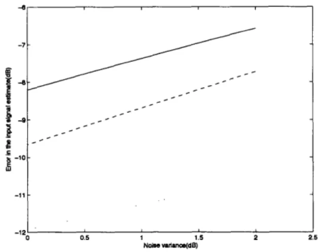
measurements. We can represent the mean square error of the input signal estimate as the sum of three error functions. We estimate the input signal using two different criteria. The first criterion minimizes only one of the three error functions, which depends only on the noise. That leads to the zero-forcing(unbiased) input signal esti-mate. This estimate is used as an initialization of the CROSS algorithm. The second criterion minimizes the entire mean square error using the previously attained initial input signal estimate and the distribution of the channel estimate. That leads to the improved input signal estimate. We can iterate the second procedure to continue to improve the signal estimate.

Chapter 5 analyzes the performance of the Least-Squares(LS) Channel Estima-tion Method and the CROSS algorithm. We implement the algorithm and perform simulations. We measure typical room audio channels by a sighted method, which estimates the channel coefficients using both the input signal and the measured sig-nals. We then artificially generate the measured signals for the simulations. For the LS method, we compare the performance of the simulation to the theoretical perfor-mance. We conclude that the channel error from the LS method is proportional to the inverse of the number of measured signal samples we use to estimate the channel and that the error is dominated by the few smallest singular value of the Toeplitz

matrix of the channel coefficients. We also perform the CROSS algorithm. We

inves-tigate the condition where the iteration process reduces the error in the input signal estimate.

Chapter 6 presents a direct method of estimating the input signal. "Direct" means that the channel coefficients are not estimated. We call this direct method the

Averaging Row Space Intersection (ARSI) method. We construct several Toeplitz matrices of the input signal that have only one row in common. Although the channel

is unknown, we can estimate the row vector space of the matrix generated from the input signal using the Toeplitz matrices of measured signals as long as the channel satisfies the diversity constraint. The performance of the estimate of the row vector

space depends on the diversity of the channel defined in Chapter 3. Since the Toeplitz matrices of the input signal have one row in common, the intersection of the row vector spaces of the Toeplitz matrices determines the common row to within a constant multiplication factor. The intersection of the estimated row vector spaces, in the noiseless case, determines and, in the noisy case, estimates the one dimensional row vector space generated by the input signal sequence. The support of the inverse channel filters determines the Toeplitz matrices of the measured signals to use. In fact, the vector of the output sequence of the inverse channel filters can be represented as a linear combination of the rows of a Toeplitz matrix of the measured signals. The other Toeplitz matrices of the measured signals are used to average the noise and decrease the mean square error. As the number of taps of the inverse channel filters

is increased, the number of row spaces to be averaged is also increased, which decreases

the mean square error.

1.6 Contributions of this Thesis

The first contribution of this thesis to apply blind equalization concepts to the prob-lem of estimating acoustic source signals as measured by multiple microphones in typical room settings. Previous approaches to this problem have fused the infor-mation from the multiple sensors through an a posteriori probabilistic model. The approach here represents a new approach to data fusion in this problem setting.

In this thesis, we generalize the notion of the channel diversity. The diversity

constraint given in [1] and restated in Section 1.3.2 only applies in the absence of

noise. We define a measure of channel diversity that accounts for the presence of noise and describes the performance of the input signal estimate. Using the newly defined diversity measure, we explain the effective channel order and generalize the blind signal estimation problem.

Compared to the MMSE estimate given in [9] that assumes correct channel es-timates, the CROSS algorithm determines the optimal inverse channel filters which accounts for the inevitable errors in the channel estimates. Also, our algorithm can

deal with deterministic input signals as well as the wide-sense stationary input signals generally assumed in the data communication theory settings.

The ARSI method uses multiple row spaces of the matrix of the input signal estimated from the measured signals. The same idea is also used in direct methods

given in [10] and [11]. However, under a fixed support of the inverse channel filters, our

algorithm, the ARSI method, uses more row spaces than the other algorithms. Since our algorithm use more vector spaces for the intersection, the error in the presence of

Chapter 2

Background

In Section 2.1, we rewrite the SIMO FIR signal model (1.1) in a matrix form. This matrix form is used in the remainder of the thesis. In Section 2.2, we introduce a

naive approach of the order estimation. We then summarize some existing order esti-mation methods. In Section 2.3, we summarize the Least Squares(LS) blind channel estimation method and the distribution of its estimates. In Section 2.4, we present a

definition of singular value decomposition (SVD) that we use in the remainder of the

thesis.

2.1 Signal Model in a Matrix Form

2.1.1

Notation

With q channels let:

Yi [n] y[n] = [yq n] win] Wq [n]

Xk[n] = [x[n] yk[n] = [y[n] Wk[n] = [w[n] Yi [n]

*-- y[n+k]]=

·

.. y[n + k]

· ' Wq[n

+ k]

h[n] = '

Toeplitz

hq[n]

+

1

x

N

+

K

+

1

block

matrix:

TN(h) is a q(N + 1) x (N + K + 1) block Toeplitz matrix:

TN (h) = h[O] h[l] ... h[K] 0 o h[O] h[l] ... h[K] ... 0 h[O] h[l] 0 h[K]

where N is an argument that determines the size of the Toeplitz matrix.

2.1.2 Equivalent Signal Models

In this section, we represent the SIMO FIR channel model (1.1) in a matrix form. We can rewrite the signal model (1.1) in a matrix form as:

(2.1) y[n] = h[O]x[n] + ... + h[K]x[n - K] + w[n].

That is,

x[n]

y[n] = [h[O] ... h[K]] +w[n] (2.2)

x[n - K]

We can increase the number of rows using the block Toeplitz matrix TN(h) to make the matrix of the channel, TN(h), have at least as many rows as columns. For safety, we choose N > K so that TN(h) is a full rank and left-invertible matrix. It

is proved in [17] that the Toeplitz matrix is left-invertible if N > K and the channel

satisfies the diversity constraint.

For any N > 0,

y[n] x[n] w[n]

[

.] = TN(h) j +

..

y[n - N] x[n- N-K] w[n- N]J

We can also increase the number of columns to make the matrix of x have more columns than rows. Then, from the assumption on the linear complexity of the input signal, all the rows of the matrix of x will be linearly independent.

For any k > 0, y[n] ... y[n + k] _x[n..] ... x[n + k]

= TN(h)

+

y[n-N] ... y[n + k-N]

x[n - N -K] ... x[n + k - N -K]

w[n-N] ... w[n+k-N]]

that is,

= TN(h) +

L

K] k[n-N]

where Xk[n] is the 1 x (k + 1) and yk[n], Wk[n] are the q x (k + 1) matrices defined previously.

2.2 Order Estimation

Many channel estimation methods such as the Least-Squares method [5] and the Subspace method [6] require knowledge of the exact channel order. Direct signal

estimation methods [10] [11] also need to know the channel order in advance. Linear prediction channel estimation methods given in [3] and [18] require only knowledge

of the upper bound of the channel order. However, in those method, the input

symbols need to be uncorrelated, which does not hold in many practical situations.

Without assuming uncorrelatedness or whiteness of the input signal, every algorithm

that we have found requires the exact knowledge of the channel order. The channel

order needs to be estimated within the channel estimation or direct signal estimation algorithms.

Generally, many channel order estimation methods have the following form: 1. Determine the possible range of the channel order

2. Construct an objective function

3. Find the channel order that maximizes or minimizes the objective function by calculating the objective function for each possible channel order in turn. The Joint Order Detection and Channel Estimation method given in [7] uses an upper bound of the order to preprocess and estimate the order and channel

simulta-neously. However, also in that method, the value of an objective function for each possible value of the channel order is also calculated.

In this section, we present a naive approach and briefly summarize the idea of the existing algorithms. We then use the estimated order to estimate the channel coefficients using the Least-Square channel estimation method.

2.2.1 Naive Approach: Noiseless Case

We pick N > K and assume that the channel diversity constraint is satisfied so that the channel matrix TN(h) has at least as many rows as columns and TN(h) is left-invertible. Assume enough linear complexity of the input and let k be a large number that makes the rows in the matrix of the input signals linearly independent and then, in the absence of noise, the rank of the matrix of the measurement signals is the same as the number of rows in the input matrix. That is,

k[n] Xk[ n]

rank

'

= rank

'

= N + K + 1.

Yk[n- N] Xk[n- N- K]

(2.5)

We can determine the order of the system by of the measurements as

K = rank

(

However, in a noisy case, rank

in the matrix. C

calculating the rank of the matrix

-N-1

= q(N + 1), the number of rows

2.2.2 Effective Channel Order Estimation

In many practical situations, a channel is characterized by having long tails of "small" impulse response terms. As presented in [14], to estimate the channel coefficients, we should use only the significant part of the channel. Otherwise, the problem of estimating the channel is ill-conditioned and the performance of channel estimation methods becomes very poor.

We summarize the effective channel order estimation methods developed. We can categorize the order estimation methods into the following two cases.

Direct Methods: Using Singular Values of the Matrix of the Measured

Signals

The order of the channel can be estimated using the singular values of the matrix

of the measured signals. Let i be the ith eigenvalue of the matrix of the measured signals,

C

These eigenvalues can be used to determine approximately the rank of the matrix so that we can determine the order from equation(2.6). Objective functions are con-structed and the rank is determined as the value of rank minimizing these functions. We present here three different objective functions used. In [13], it is assumed that the measured signals form Gaussian processes, information theoretic criteria is used,

and two approaches called AIC and MDL are used.

1 (qN-r)(k-1) qN qN-r AIC(r) = -2log _ =rN+ + 2r(2qN - r) (2.7) (qN-r)(k-1) MDL(r) = -210og

g

(

)

+ -r(2qN

2

)I

In practice, the Gaussian assumption may not hold, weakening the basis of these methods. Furthermore, AIC method tends to overestimate the channel order.

In [14], the following function called Liavas' criterion is used.

LC(r) = r-2r+l' A

<

(2.9)

Joint Methods

Unlike the previous three methods, based on the singular values of the matrix of the measured signals, the following two methods seek to determine the order and channel coefficients jointly. The method given in [7] performs joint estimation. In this method, the order of the channel is initially overestimated. Denote the overestimate as 1. Then, by Least Squares Smoothing (LSS ) [19] the column space of Tl_K(h)T is estimated and the orthogonal vector space of the column space is determined. The objective function is calculated as the the minimum singular value of the block Hankel matrix of the orthogonal vector space. The argument of the objective function is related to the size of the block Hankel matrix. The order is determined as the value minimizing the objective function.

When the channel order is correctly detected, Least Squares (LS) [5], Signal Sub-space (SS) [6], and Least Squares Smoothing (LSS) [19] perform the channel estima-tion better than the joint channel and order estimaestima-tion method.

The method given in [15] uses the channel estimate to improve the order estimate. The method overestimates the order of the channel via the AIC method and then estimates the channel using channel estimation methods such as LS [5], SS [6], and LSS [19] at the given order. In theory, a transfer function of each estimated filter is a multiple of a transfer function of the real filter and the ratio of them is the same for any filter. By extracting out the greatest common divisor, the real channel is estimated and also the effective order is calculated. However, this method can be applied only to the case of two measurements.

2.3 Least Squares Blind Channel Estimation Method

In this section, we summarize the LS channel estimation method[5] and its

perfor-mance derived based on the proof of Theorem 13.5.1 in [16].

2.3.1 Notation

yi[N- K + 1]

2.3.2 Algorithm

In the noiseless case, for any 1 < i, j < q, we can see

yi * hj = (x * hi) * hj = (x

hj) * hi = yj * hi.

Yi[N]hj = Yj[N]hi. Yi [K] Yi[K + 1] yi[N - K] ... yi [2K]

'.

yi[2K+l]

From equation (2.14), we can make a linear equation of the form:

Yh = 0 (2.15)

where Y is formed appropriately[5].

For example, for q = 2, the matrix, Y, is

Y = [Y2[N] -Y 1 [N]] (2.16)

and, for q = 3, the matrix, Y, is

Y2[N] -Y 1 [N] 0

Y = 3[N] 0 -Y[N] (2.17)

0 Y2[N] -Y 1 [N]

In the noisy case, each entry of the matrix, Y, has a signal component and a noise component. Thus, we can represent the matrix Y as the sum of two matrices Y, and Yw,. One is associated with the filtered input signal and the other is associated with the noise.

The channel coefficients satisfy

Yh = 0. (2.18)

Since we cannot separate Y, from Y, we estimate the channel as the vector that minimizes I Yhll given that I hl = 1. That is, h is given by the right singular vector associated with the minimum singular value of the matrix Y. The details are given

in [5].

2.3.3

Performance

Let hi be the estimate of hi. We assume that the input signal, x, is a determinis-tic signal and the noises, wi, are i.i.d zero-mean Gaussian random processes. The

distribution of the channel estimate using the LS method is derived in Appendix A

where we modify the proof of Theorem 13.5.1 given in [16]. The derived asymptotic distribution is

h q(K+1)-1

h= hi- + ciui (2.19)

where ci is a zero-mean Gaussian Random Variable with variance

Zq(q-1 )2(A? + )q(q-1)a2)

2 2 (2.20)

(N - 2K)A

and Ai and ui are the ith singular value and the it_{h right singular vector of the matrix}

VN -2Yx The c are independent of each other.

2.4 Singular Value Decomposition (SVD)

We use the following definition of the singular value decomposition in the remainder of the thesis. This definition is used in MATLAB function svd.

Definition of SVD

Any m x n matrix, A, can be written as

A = UV* (2.21)

where U is a unitary matrix of dimension m x m, V is a unitary matrix of dimension

n x n, and E is a m x n diagonal matrix, with nonnegative diagonal elements in

decreasing order. The matrix V* is the conjugate transpose of V.

For a real matrix A, the unitary matrices, U and V, also become real matrices, the columns of U form an orthonormal basis of Rm_{, the columns of V form an}

Chapter 3

Diversity of the Channel

In Chapter 1, we mentioned that, in the absence of noise, to have a solution to within a constant multiplier to the channel identification problem, the transfer functions of the channel should have no common zeros. This is called the channel diversity constraint. However, in the presence of noise, to our knowledge, a good measure of the performance of the input signal estimate as affected by the characteristics of the channel coefficients has not been defined yet. In this chapter, we define a measure of the diversity of the channel, D(hl, h₂,... , hq), to characterize the channel based on

the following desired properties.

3.1 Properties

1. Diversity of the identity channel is one.

D(6[n]) = 1 (3.1)

2. Diversity is zero if and only if the transfer functions of the channel have one or more common zeros.

3. As a corollary, diversity of one filter with at least two taps is zero since the

transfer function of the filter is itself the greatest common divisor of the transfer function.

D(h1) = 0 (3.3)

4. A pure delay in any channel does not change diversity.

D(hl[n], * , hi[n - k], , hq[n]) = D(hi[n], , hi[n], ... , hq[n]) (3.4)

5. For any constant c,

D(chi, ch2, ,chq) = IcID(h, h2, , hq) (3.5)

6. An additional measurement may increase and cannot decrease diversity.

D(h, ... , hq) < D(h, , hq, hq+l) (3.6)

3.2 Definition of Diversity

Property 2 says that diversity is zero if and only if the channels do not satisfy the

noise free channel diversity constraint. That is, transfer functions of the channel

have one or more common zeros. Suppose the transfer functions of the channel has a

common zero and let z = a be the common zero of Hi(z), ... , Hq(z). In other words,

Hi (a) = ... = Hq(a) = 0. In the absence of noise, the measured signals generated

by the input signal, x[n] = an, are all zeros. Thus, there is no way to determine the

component of the input signal with the form x[n] = can. Mathematically speaking, we can represent any signal as the sum of the following two signals. One signal belongs to the the vector space ca nc is a complex number} and the other signal is orthogonal to this vector space. If the transfer functions of the channel have a common zero at

z = a, then we cannot determine the component of the input signal belonging to the

One possible definition of diversity, which satisfies the desired properties, is the

minimum ratio of the energy of the measurement signal to the energy of the input signal. Intuitively, this measures the worst case amplitude response of the channel. The input signal associated with this worst case amplitude response is the most difficult signal to determine in the presence of noise. The diversity measure proposed

is:

D(hl, .

hq) _ min

.

- ({(hl

* x)[n]2

+

+ (hq

* x)[n]

_}

₍₃₇₎

X E00 -,Z- c x[] (3.7)

In Appendix B, we prove that this definition satisfies all the properties given in the previous section.

3.3 Diversity with Finite Length Signals

The definition of diversity in the previous section assumes that the length of the input signal is infinite. In practice, however, we can observe only a finite number of samples from the measurements. In this section, we reformulate the definition of diversity when only a finite number of samples are available.

Suppose that the channel is known. We measure the samples from index n - N to index n: y[n - N],... ,y[n]. From (2.3), the measurement signals satisfy the

following equation:

y[n] x[n] w[n]

.

j

=

.

+

.

(3.8)

y[n- N]] x[n- N-K] [w[n- N] Let's decompose TN(h) using singular value decomposition (SVD) as

where

U =[ul u2 ... Uq(N+l)] , (3.10)

V [v1 v2 *.. vN+K+I] . (3.11)

Each ui, vj is a column vector of length N + K + 1. Let Ai be the ith singular value, i = 1,... , N + K + 1, ordered in descending magnitude. From equations (3.8) and (3.9), we can reorganize our channel as q(N + 1) parallel channels as, for

1 < i < N+K+1,

x[n] w[n] y[n]

AiViT '

+ UiT

'

uiT

,

(3.12)

x[n- N-K] w[n- N]J y[n- N]J

for N + K + 2 < i < q(N + 1),

w[n] y[n]

uLT J = uiT n N (3.13)

w[n- N] y[n- N]

The signal to noise ratio (SNR) of the output of each parallel channel depends on the singular value of TN(h), Ai, which is the gain of each channel. The minimum singular value, AN+K+1, which is the smallest gain, determines the accuracy of the

estimate when the worst-case input signal, whose components are zero except for the component in vi direction, is applied. If AN+K+1 is small, we need to greatly amplify

the noise to estimate the component of the input signal in VN+K+lT direction.

y[n]

In the absence of noise, the minimum ratio of the magnitude of ' to

y[n- N]

x[n]

the magnitude of

j

of the channel becomes

Diversity = lim N+K+1 (TN(h))

N-oo (3.14)

In Appendix B, we prove the convergence of limN. AN+K+1 (TN(h)).

3.4 Examples: Small Diversity

In this section, we present three different kinds of channel that have small diversity.

3.4.1 Common Zeros

Let He(z) = GCD{Hi(z), ... , Hq(z)}. Let the transfer functions of the channel have one or more common zeros and thus Hc(z) is not a constant. Then, there exist

h,1' *, hq such that hi = h * h, · · , hq = h * hq. Let fK be the order of the channel

bh1," ,hq. Then, < K.

Each row of the Toeplitz matrix, TN(h), satisfies the following equation:

[o ... h h] i [K] ... ] =

[o

..-

N +

K

Then, the Toeplitz matrix, TN(h), can be written as h[O] h[l] ... h[K] 0 ... 0 h[O] h[l] ... h[K] 0 ... ... 0 h[O] h[1] ... h[K] i[o] [1] ... hi[K] 0 ...

o h[o] []

[]

[]

...

Thus, the matrix, TN(h), is not a full rank matrix:

rank(TN(h))

< N + K + 1 < N + K + 1.

If the transfer functions of the channel have one or more common zeros, since TN(h) is not full rank and then the minimum singular value of the matrix TN(h),

AN+K+1 (TN(h)), is zero. Thus, the diversity of the channel is zero.

3.4.2

Filters with the Same Stop Band

Let the filters have the same stop band: w E [wl, w2]. By that we mean the frequency

responses of the filters satisfy, for w E [wl, w2],

IHi(e)lI < E, (3.18)

where e is a small positive number.

Let:

the matrix D be the (N + K + 1) x (N + K + 1) diagonal matrix whose entries are

Dn,n = e-jWln for n = 1,--. ,N+ K+1, (3.20)

the matrix F be the (N + K + 1) points DFT matrix whose components are

=

for n =

for

1,.

. ,N+K+landm=l,...

,N+K+1,

e-J

ei

Let r[n] be a signal with support [0, N + K]. Let r be a row vector with length

N+K+1:

r = [r[0] r[1]

... r[N + K]]

-By multiplying DF to the row vector, r, we can determine the value of Fourier Transform of the signal, r[n], at frequencies w = w1 + N+K+1 for k = 0,- - , N + K.

That is,

[r[O] r[l]e-'wl ·..

r[N

= [R(ej )

Thus, the row vector of TN(h) multiplied by DF is

(3.21)

(3.22)

(3.23)

rDF =

[0 ... 0 hi[O] hi[1] ... hi[K] 0 .. O]DF =

[Hi[O]e i N+K+1 +w)m H [l]e-j(N+K+w)m Hi[N

+

where m is the number of consecutive zeros in the beginning of the the row vector.

Therefore, all the entries of TN(h)DF can be written as the frequency responses

Hi[k] multiplied by a unit norm complex number.

H1[0] Hq [0] Hl [O]e j(N+T +-1)1 Hq[O]ej( + r + ~)l H1[OJ]ej( N+ 21 1 ) (N-1) Hq [O]e j( +1 +1 )(N-1) TN(h)DF = H1i(1] Hq[1] H1[j(N+le + +1)1 Hq[l]e j( N+K+1 +.)l H1[l]e ( N+K+1 +j)(N-1) [l]e( +K+ +- 1)(N-1) Hq [1]. -RF ·,,. H [N + K] .. HqN+ +K] H1[N f K]eH l ( N+K+1+w1)1 Hi[N+K]e+ (j N--. +Wl)) ..

H[N

+

K]e

1)(N1

2

Since IHi[[0] = IHi(eiw)l < c, all the components of the first column have

magni-tude less than . Thus, the magnimagni-tude of the first column is less than /q(N + 1).

Therefore, the smallest singular value of TN(h)DF is less than /q(N + 1)E. Since all the rows of F are orthogonal to each other and they have the same norm x/N + K + 1,

VN+K+1 F is an unitary matrix. The matrix D is also unitary. Since the multiplying

by a unitary matrix does not change the singular values, the singular values of TN(h)

are the same as those of 1 T N(h)DF. Therefore, the smallest singular value of

3.4.3

Small leading or tailing taps

The minimum singular value is less than or equal to the magnitude of any column:

AN+K+1 (TN(h)) = min IITN(h)v< IITN(h)ill (3.25)

where TN(h)i is the ith column of TN(h).

Thus, the diversity of the channel is less than or equal to the magnitude of the first column and the last column:

D(h, hq) q, /h[0] 2+ +hq[O]2 (3.26)

D(hl, , h

< vhl[K]

+ hq[K]

(3.27)

Therefore, if all of the multiple measurement channel simultaneously have small leading or tailing taps, the diversity of the channel is also small.

3.5 Effective Channel Order Revisited

As given in [12], given that the input signal is white, the performance of the LS (least squares) channel estimation method[5] and SS (signal subspace) channel estimation method[6] degrade dramatically if we model not only the "large" terms in the channel

response but also some "small" ones.

As shown in the previous section, the channel that has small leading or tailing taps is one of the channels that have small diversity. We have explained here using our extended concept of diversity why modeling not only significant terms but also insignificant terms decreases the performance of the LS channel estimation method.

We show, in Appendix A, if the diversity of the channel is small, then with a white input signal and white additive noise, the performance of the LS channel estimation method become very poor. We also show that if the diversity of the channel is large, then with a white input signal and white additive noise, the error of the channel

estimate using the LS channel estimation method becomes very small.

We can increase the diversity of the channel by ignoring the insignificant part

of the channel. If we use only significant part of the channel to estimate the input

signal, the noise is not greatly amplified in the estimation process. In other words, underestimating the order increases the diversity. However, ignoring the insignificant part of the channel means that the measured signals from the insignificant part must be regarded as noise. Therefore, underestimating the the channel order increases the

noise variance. This produces an engineering tradeoff.

3.6 Diversity over a Constrained Vector Space

Symbols in the data communication problem are usually i.i.d, so the power spectral

density of the measured signals is nonzero over all frequencies. However, acoustic signals, for example, music signals, are usually low frequency signals. In this case, we

have a prior knowledge of the input signal: all the signals are the elements of a certain vector space. Also, sometimes, our interest is in estimating the input signal over a certain frequency band. In this section, we generalize our definition of the diversity and propose a new problem statement.

Define diversity over a vector subspace V as

Dv(hl,... hq)= lim min TN(h)v (3.28)

N-toovEV Vii11

In Section 3.5, we mentioned that by ignoring the insignificant part of the channel, the diversity can be increased. We can also increase the diversity by constraining our interest in estimating the input signal. For example, let the transfer functions of the channel have common zeros and He(z) = GCD{Hi(z), ..., Hq(z)}. As is shown in Section 3.4.1, the diversity D of this channel is zero. Choosing V = {vlh, * v = O}I makes the diversity Dv nonzero since the measured signals cannot be zero with nonzero input signal taken from this subspace. Estimating an input signal component

input signal over the entire signal space will greatly amplify the power of the noise. We can generalize our problem of blind signal estimation as follows:

Generalized Problem Statement:

Given the measured signals, estimate the component of the input signal on a certain vector space which minimizes the mean square error over the vector space.

Chapter 4

Linear MMSE Signal Estimate of

the Input given the LS Estimate of

the Channel: The CROSS

Algorithm

4.1 Mean Square Error of the Input Signal

Esti-mate

Using the LS channel estimation methods, we can have the estimate of the channel prior to estimating the input signal. As is written in Section 2.3.3, the asymptotic estimate h can be written in the following form:

h= -+

e

llhll

where e = i -1 C) iUi.

A coefficient, ci, is a zero-mean Gaussian random variable with variance

q(q-1) + _2_( _q(q--1) 2)

(N - 2K)A4

(4.1)

and Ai and ui are the ith singular value and the ith right singular vector of the matrix

1N Y. The ci are independent of each other.

For simplicity, we assume that I hi I = 1.

The mean square estimate error of x[n] (1.6) can be written as

= [1 T ,E ([4n] - n)2]

T

n=l

E [(f * y +

*

+ fq *

yq)[n]

- x[n]}2]

(4.3)

Let

g =f

*hi +

+ fq*hq.

(4.4)

When we estimate the channel using a large number of the samples of measured signals, we can regard our channel estimate as a function of measured signals' samples. Since, for all i = 1, ... , q and n, the noise samples, wj[n], are independent to each other, the dependence of the error of the channel estimate on any particular noise

sample is negligible. Also, if yj [n] is not the sample used to estimate the channel, wj [n]

is independent to the channel estimate. Thus, we assume that, for all i,j = 1, ... , q

and m, n, ei[m] and wj[n] are uncorrelated and we split the expected value inside the summation as

E [{(fl * Yl + - + fq * yq)[n]

- x[n]}2]

E [{(g *

x)[n]

[{(f * e +

...

+E [(fi * w + + fq * wq)[n]

_{] .}

_(4.5)

Then, the mean square error, , becomes

where 61 =

T

=

E

(f*

w

+.

+ fq*wq)[n]

,

(4.7)

=-E

T

{(

* el +

+

fq

* eq)

* x}[n]2

(4.8)

The second term, 62, can be simplified as

62 = E

[E=

=

[

E=l(E,-

fi[=f

m]wl[n - m]

+ fq[m]wq[n

m])2]

1 T n= M=

ETn=l

Elm=-

_

fi[m]

_E[wl[n

_{- m]2]}

₊

_{+ fq[m]}

_E[wq[n

_-

_m]2]

U2

If the estimate is unbiased, the expected value of the estimate should be equal to the input signal:

x = E[x] = g*x-E[(f *el +- +fq*eq)*x]+E[fi*wl+ *

= g*x (4.9)

That is, for an unbiased estimate, g = 6. This constraint is called the zero-forcing condition from its history in data communications. In this case, the first term of the

error e1 = 0.

If the estimate of the filter coefficients are correct, then e = 0, so 63 = 0.

4.2 Initializing The CROSS algorithm

In Section 4.4, we will present the MMSE FIR estimate of signal that minimizes the total error, , introduced above. To make the appropriate tradeoffs, the optimal filter