Acoustic emissions in hydraulic fracturing of Barre granite

Acoustic Emissions in Hydraulic Fracturing of Barre Granite

ARCHIVES

by

Qiuyi

JUL 02 2015

University of Toronto, 2013

IBRRIESIZ

SUBMITTED TO THE DEPARTMENT OF CIVIL AND ENVIRONMENTAL

ENGINEERING IN PARTIAL FULFILLMENT OF THE REQUIREMENTS FOR THE

DEGREE OF

MASTER OF SCIENCE IN CIVIL AND ENVIRONMENTAL ENGINEERING AT THE

MASSACHUSETTS INSTITUTE OF TECHNOLOGY

JUNE 2015

@2015 Massachusetts Institute of Technology. All Rights Reserved.

Signature

Signature of Author:

redacted

Department of Civil and Environmenta Elngi eering 20 ay, 2015

Signature redacted

Herbert H. Einstein Professor of Civil and Environmental Engineering Thesis Supervisor

Accepted by:

___________Signature

redacted

r , "eifti Nepf Donald and Martha Harleman Professor of Civil and Environmental Engiheering

Acoustic Emissions in Hydraulic Fracturing of Barre Granite

by

Qiuyi Bing Li

Submitted to the Department of Civil and Environmental Engineering on May 20, 2015 in

Partial Fulfillment of the Requirements for the Degree of Master of Science in Civil and Environmental Engineering

ABSTRACT

The purpose of this work is to observe acoustic emissions (AE) generated by laboratory scale hydraulic fracturing of Barre granite specimens with single or double flaw geometry. The scope of this work covers the experimental setup and subsequent analyses of these acoustic emissions, which in essence are elastic waves generated by displacements occurring within the rock specimen. Acoustic emissions can be analysed in a number of ways, whether individually or grouped together into events when a number of emissions arrive together. Individual emissions can be analysed for their amplitude, energy, or their frequency content while the source location and source mechanism can be inferred from events. The AE data are analysed in conjunction with water pressure, high resolution images, and high speed video taken during the experiment. Section 3 of this work outlines the selection and subsequent modification of the AE acquisition system with a specific focus on capturing AE at the end of each experiment in order to compare results to high speed video. This section describes the initial equipment selection, as well as initial experiments where it was noted that crucial data were missing around the time of the fracture event. This issue was largely resolved by modifying the system parameters as well as upgrading the PC supporting the AE acquisition cards.

Section 4 of this work describes analysis of one experiment, providing an in-depth start-to-finish account of the nature of acoustic emissions at different phases of the experiment. This section also considers all of the hydraulic fracture experiments performed at different vertical loads and specimen flaw geometries, and draws some tentative conclusions regarding hydraulic fracturing in granite.

Thesis Supervisor: Herbert H. Einstein

ACKNOWLEDGEMENTS

"It's the job that's never started as takes longest tofinish" - J.R.R. Tolkien

If I had my way, I would wake up every day at noon, sit around drinking tea and ultimately get no work done. Clearly, that has not entirely been the case. This is thanks to the people around me that motivate me to be...well... a useful human being. I would like to thank my family for having my best interest at heart all these years, my friends for putting up with me and my eccentricities, and my lab mates for our endless discussions on life, the universe, Joe coffee and DOTA 2

(occasionally rocks and fractures get brought up). Thanks of course go to Professor H.H. Einstein and to Dr. J.T. Germaine for being the fountains of knowledge and insight that they are. Finally,

I would like to thank Total S.A. for sponsoring my work, and the annoying bugger who kept poking

CONTENTS

1.3 Relation to seism ology... 14

2.0 Background...15

2.1 Term s and definitions... ₁₅

2.2 AE Analysis techniques... 22

2.2.1. Localisation... 23

2.2.2. _{Source characterisation - M om ent tensor ... 31}

2.2.3. Source characterisation - Polarity m ethod ... 42

2.3 Previous Experim ental W ork... ₄₃

2.4 Setup of Hydraulic Fracturing experiments...49

3. Equipm ent... ... 3.1 Equipm ent Selection...--- . ... ... 53

3.11. Sum m ary.. ... 53

3.1.2. Introduction...---.----.. ... . .... ... .. 53

3.1.3. Equipm ent description ... 54

3.1.4. Prelim inary calibration experim ents - April 2014... 55

3.1.5. Equipm ent selection ... 68

3.2 Calibration tests perform ed in July 2014... ₇₄

3.2.1. Steel rod tests... ₇₄

3.2.2. _{Incidence angle ... 77}

3.2.3. Steel localisation ... 80

3.2.4. _{3D sensor array... 83}

3.3 Acoustic Em ission System Issues...88

3.3.1. Observed problem s... 88

3.3.2 Attem pts to understand the problem ... 9 1 3.3.3 Solutions attem pted... 99

3.3.4 Chassis upgrade ... 105

3.3.5 PCI-2 lim itations...107

3.3.6 Further solutions ... 10

3.4 Experim ental Setup of AE Equipm ent... 109

3.4.1 Data acquisition system ... 110

3.4.3 Sensors ... ill

4-o Results ... 117

4.1. Analysis of hydraulic fracture Of 2a-30-9o-VL5-INC5-C ... 117

4.1-1. Experim ental Procedure ... 117

4.1.2. Experim ent Overview ... 118

4.1-3. Localisation ... 120

4.1-4. Energy Analysis ... 122

4.1-5. High resolution im ages ... 124

4-1.6. High Speed Video ... 125

4.1-7. W aveform s near to tim e of failure ... 128

4.1.8. Power spectrum analysis ... 129

4.1-9. P-wave velocity ... 131

4.1-10. M om ent tensor analysis ... 134

4.2. Sum m ary of all hydraulic fracture experim ents on granite ... 139

5.0 Sum m ary and Conclusion ... 145

6.o References ... 147

Appendix A: Dialogue with Dr. Pollock ... 149

Appendix B: Param etric connector ... 153

Appendix C: High speed cam era trigger ... 156

Appendix D: Localisation using the double difference m ethod ... 16o Appendix E: Data for all experim ents ... 167

2a-3o-o-VLo-INC5-B ... 167 2a-3o-o-VLo-INC5-C ... 169 2a-3o-o-VL5-INC5-A ... 171 2a-3o-o-VL5-INC5-C ... 173 2a-30-3o-VLo-INC5-C ... 175 2a-30-3o-VL5-INC5-B ... 177 2a-30-3o-VL5-INC5-C ... 179 2a-3o-6o-VLo-INC5-C ... 181 2a-3o-go-VLo-INC5-B ... 183 2a-3o-go-VL5-INC5-C ... 185 2a-30-12o-VLo-INC5-B ... 187 2a-30-12o-VL5-INC5-B ... 189 3o-VL5-INC5-B ... 191 3o-VL5-INC5-C ... 193

Appendix F: P-wave velocities ... 195

2a-30-30 -3 o-B ... 199

2a-30-30 -30 -C ... 200

Appendix H : Uniaxial Test on granite ... 202

LIST OF FIGURES

Figure 2 -Example of an acoustic emission ... ₁₅

Figure 3 - Schematic representation of acoustic emission...16

Figure 4 - (Left) AE DAQ system logic... ₁₇

Figure 5 - An exam ple of an AE event... 18

Figure 6 - Amplitude over time for all sensors ... 19

Figure 7 - Sam ple w aveform ... 21

Figure 8 - (Top) Illustration of P-wave... 22

Figure 9 - Schematic of the travel time... 23

Figure 1o - Sam ple w aveform arrival... 24

Figure 11 - Schematic of the waveforms observed ... 25

Figure 12- Illustration of AIC... ₂₇

Figure 13 - Residual values for the arrival times ... 28

Figure 14 - Illustration of double difference method... 30

Figure 15 - Schematic transverse view of a crack showing ... 32

Figure 16 - Example of a source-time function... ₃₃

Figure 17 - Moment tensor components given a unit cube... 34

Figure 18 - Schematic of a source in relation to the sensor... 35

Figure 19 - Physical representation of ratios X, Y, Z. ... 38

Figure 20 - Schematic of a penny shaped crack ... ₃₉

Figure 21 - Experimental crack geometry... ₄₀

Figure 22 - Schematic showing plane waves ... ₄₁

Figure 23 -Illustration of polarity technique... ₄₃

Figure 24 - Stress-displacement curve of (Lockner, et al. 1991)... ₄₄

Figure 25 - Localisation of AE events at different stages ...---... ₄₅

Figure 26 - (Right) Energy release at different locations ... 46

Figure 27 - Experimental setup of (Shigeishi and Ohtsu 1999)... ₄₇

Figure 28 - Results of 2D moment tensor ... 48

Figure 29 - AE close to tim e of failure. ... ₄₉

Figure 30 -a) Front and b) side view of the water pressure device...51

Figure 31 - Picture of experimental setup. .... ..---... ... 52

Figure 32 - Schematic of hydraulic fracturing experiment... 52

Figure 33 -Response from pencil lead break ... 56

Figure 34 - Response from ball drop .--..---... 57

Figure 35 -Response from ball on pin... _{...- 57}

Figure 36 - Power spectrum of ball on pin test on gypsum with Nano3o sensor... 58

Figure 37 - Power spectrum of ball on pin test on gypsum with R6i sensor ... 58

Figure 38 -Power spectrum of ball on pin test on gypsum with R3a sensor ... 58

Figure 39 -Response on granite ...-... ... 59

Figure 40 -Response on m arble... 6o Figure 41 -Response on shale ... 6o Figure 42 -Localisation accuracy on intact sample. ... ₆₁

Figure 43 - Hypothetical 3 sensor network ... 62

Figure 45 -Localisation accuracy of 2a-30-120 granite sample... 64

Figure 46 - Contour plot showing localisation error in Figure 45... 65

Figure 47- Sam ple w aveform ... 66

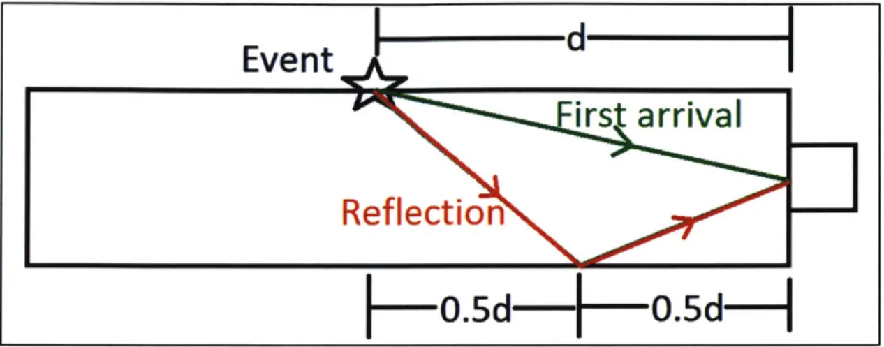
Figure 48 -Calculation for arrival of the reflection... 67

Figure 49 -First half wave of a hit... 70

Figure 50 -Frequency response curves for VS45-H (L) and VS150-M (R) sensors...71

Figure 51 -Frequency response of AE1045S sensor ... 71

Figure 52 -Micro3o (L) and Micro3oF (R) response curve ... 72

Figure 53 - Schematic showing setup for AST tests on a steel rod ... 74

Figure 54 - Waveform produced by the pulsing sensor...75

Figure 55 -Waveform detected by receiving sensor... 76

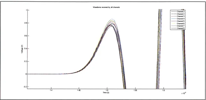
Figure 56 - Waveforms detected by all sensors ... 76

Figure 57 - Reception of AST pulse by all 8 sensors: zoomed into first arrival...77

Figure 58 -Sensor and artificial source locations for incidence angle test ... 78

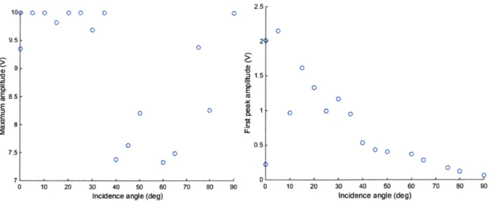
Figure 59 - (Left) Maximum waveform amplitude as a function of incidence angle. ... 79

Figure 60 - Sensor layout for second incidence angle experiment... 79

Figure 61 - Plot of time error for an AST pulse...8o Figure 62 - Localisation for the first sensor configuration...81

Figure 63 - Localisation for second sensor configuration ... 82

Figure 64 - Sensor locations for 3D localisation... 83

Figure 65 - Plan view (along x axis in Figure 64) ... 84

Figure 66 - A section view of Figure 65 along the Y axis. ... 85

Figure 67 - Schematic of experiment to determine accuracy of localization...86

Figure 68 - Planview localization of pencil lead breaks... 86

Figure 69 - Isom etric view of Figure 68 ... 87

Figure 70 -Amplitude of AE hits (dB) and water pressure (MPa) over time (s)... 89

Figure 71- Amplitude of AE hits (dB) and water pressure (MPa) over time (s) ... 90

Figure 72 - Time trace of 4 channels and pressure reading close to crack propagation ... 92

Figure 73 - Configuration of sensors and earphones... 93

Figure 74 - Effect of saturated AE hit rate, data from channel 1... 93

Figure 75 -Time between hits on 1 channel on a saturated signal... 94

Figure 76 -Average time between hits at different HLT's... 95

Figure 77 - The effect of HLT on the saturation time ... 96

Figure 78 - CPU usage of the computer under constant AE triggering ... 97

Figure 79 -Result from 4 sensors @ 1oMHz in a 4-core CPU... 98

Figure 8o -Critical time segment infeasibility of good data ... 100

Figure 81 - Event localisation from test done as per the parameters in Table 9a. ... 102

Figure 82 -Event localisation from test done as per the parameters in Table 9b. ... 103

Figure 83 - Hit amplitude over time for test corresponding to Table 9a ... 104

Figure 84 - Hit amplitude over time for test corresponding to Table 9b... 104

Figure 85 - Hits over time at 1oMHz on the new system ... 1o6 Figure 86 - Summary of CPU usage under signal saturation. ... io6 Figure 87 - a) Front and b) side view of the water pressure device...112

Figure 88 - Sensor locations ... 113

Figure 89 - Acrylic template used to position the sensors...114

Figure 90 - Sensor markings used to guide sensor bonding locations... 114

Figure 91 - Picture of the hot glue fillet ... 116

Figure 92 - Schematic showing the bonding materials ... 116

Figure 93 - Schematic illustrating the timing of high speed video...-156

Figure 94 - Example of a sampled trigger voltage drop off curve. ... 157

Figure 96 - _{The upper part of Figure 95 is shown here. ... 159}

Figure 97 - The upper part of Figure 96 is shown here. ... 159

Figure 98 - Timing of vertical load and water pressure application. ... 118

Figure 99 - a) Water pressure, AE hits, as well as events...119

Figure 100 - Localisation of events... 121

Figure 101 - Semilog plot of AE energy as a function of water pressure. ... 122

Figure 102 - Semilog plot showing the AE energy of individual hits...123

Figure 103 - Analysis of high resolution photos ... 124

Figure 104 - Left image shows the high speed frame ... 126

Figure 105 - _{Schematic images showing extent of white patching ... 127}

Figure 106 - Waveform trace on channel 4...128

Figure 107 - Same trace as in Figure 1o6, with y-axis reduced ... 129

Figure 1o8 - Waveform trace from points G to H in Figure 106 ... 129

Figure 109 - _{(Left) Power spectrum of the high amplitude waveform ... 130}

Figure 110 - P-wave velocity evolution ... 132

Figure 111 - _{P-wave velocity measurement ray paths ... 133}

Figure 112 - _{Effect of confining pressure and saturation...133}

Figure 113 -Moment tensor decomposition values...134

Figure 114 - _{The last 70 seconds of Figure 113 showing behavior close to failure...135}

Figure 115 - Shear events in 2a-30-90-VL5-INC5-C ... ₁₃₆

Figure 116 - Tensile events in 2a-30-90-VL5-INC5-C...137

Figure 117 - Polar histogram of opening or normal direction of shear events ... 138

Figure 118 - _{Polar histogram of the opening direction of tensile events. ... 139}

Figure 119 - Maximum water pressure and total emitted AE energy ... 141

Figure 120 - Plot showing energy distribution near to failure for all specimens. ... 142

Figure 121 -Plot showing AE hits at the low energy range for all experiments. ... 143

Figure 122 - Events localized for the given dataset using AIC arrival picking ... 163

Figure 123 - _{Localisation on the same data as Figure} 122...164

Figure 124 - Localisation results comparing the double difference and traditional methods. .. 165

Figure 125 - Localisation results comparing the double difference method ... ₁₆₆

Figure 126 -Stress strain graph and AE energy of 2a-30-30-30-B on Opalinus shale...199

Figure 127 -Largest waveform observed over the course of the experiment. ... ₁₉₉

Figure 128 - High resolution images, stress strain graph and AE energy of 2a-30-30-30-C.... 200

Figure 129 - Largest waveform observed over the course of the experiment... 201

Figure 130 - Cumulative hits for uniaxial compression on granite ... 202

Figure 131 -Stress-strain and amplitude plot for uniaxial compression on granite _{... 203}

Figure 132 - _{Localisation results for Uniaxial test on granite... 204}

1.0

INTRODUCTION

1.1 MOTIVATION

The main motivation for this work is to develop a system to capture acoustic emissions from experiments currently performed by the rock mechanics group at MIT. Acoustic emissions are elastic waves generated from rapid energy release within a material. These elastic waves propagate through the material, and can be observed using electro-mechanical transducers that can convert the small displacements observed at the surface into voltage changes that are sampled

by a data acquisition system.

The experiments performed by the rock mechanics group impose various loading conditions on rock specimens with pre-cut flaws such as shown in Figure 1. The goal is to gain insight into crack initiation, propagation and coalescence, as well as white patching which appears to correspond to the development of a process zone. Stress, strain and hydraulic pressure data are gathered throughout the experiment, and are used in conjunction with high resolution and high speed photography. The main limitation of analyses using images is that only surficial behaviour is observed, and it is hoped that acoustic emissions will provide information as to whether the same phenomena are observed at depth.

160 140 S4 S5 120 100 S3 S6 E E80 60 S2 S7 40 20 S1 S8 t 0* - -0 20 40 60 80 x (mm)

Figure 1- Typical granite test specimen. Left side shows a schematic of the specimen and flaw geometry

as well as sensor locations. Right side shows a photo with sensors and granite specimen.

1.2 BRIEF HISTORY

This section is largely adapted from (Drouillard 1996). The earliest recorded observation of acoustic emissions was in Arabian alchemist Geber's work in the 8th century. He noticed that during smelting, tin would produce a "harsh sound" that later became known as tin cry and that iron would "sound much" during forging. It is possible these sounds would have been noticed as early as the Bronze age (around 3500BC), when man first learned to smelt tin. Other metals such as cadmium, magnesium and zinc were also noted to produce audible acoustic emissions by the mid-1_{9th century. By the 1930s a number of studies established a clear correlation between} mechanical twinning in metals and audible sounds whose frequency depended on the geometry of the specimen.

In parallel, advancements in technology for measurements of high frequency, small amplitude oscillations allowed one to study acoustic emissions. These included the acoustic horn in the 17th

century, the stethoscope in 1816, and the development of electro-mechanical devices in the early

2 0th century that facilitated conversion from mechanical motion to an electrical signal.

One of the pioneers of the field was Josef Kaiser, who performed a number of tensile tests on metal alloys in the late 1940s and 1950s _{at the Technische Hochschule Munchen in Germany} (Tensi 2004). He studied the variation of amplitude and frequency in relation to the stress-strain curve, and one of the most notable observations was the phenomenon that the production of acoustic emissions were irreversible, much like plastic strain. This implies that fewer emissions are observed until the historical maximum stress of a material is reached, and is now known as the Kaiser effect.

1.3 RELATION TO SEISMOLOGY

Seismology is the study of earthquakes, which are primarily understood through study of the elastic waves that are propagated through the Earth and detected at some distance from the source (Grosse and Ohtsu 2008). This is entirely analogous to acoustic emissions, where sensors gather

information regarding elastic waves generated from energy releases at depth. The main difference between the two fields lies in scale. Where earthquakes occur kilometres within the Earth, acoustic emissions operate at most on the metre scale, and as a result tend to be much lower in amplitude and higher in frequency than that observed in seismology. These factors require acoustic emissions equipment to have higher voltage sensitivity and resolution to be able to observe smaller events, as well as operate at higher sampling rates to be able to capture the higher frequency events.

2.0

BACKGROUND

2.1 TERMS AND DEFINITIONS

A large portion of this is adapted from the Physical Acoustics Corporation user manual (PAC

2007).

Acoustic Emission (AE): an elastic wave generated from rapid energy release within a

material. An earthquake is effectively a large acoustic emission. An example is given in Figure 2.

0.2 0.15 0.1

III

_.

h

p

Figure 2 -Example of an acoustic emission from granite hydrofrac test 2a-30-60-VLo-INC5-C

Acoustic Emission System: a system that facilitates the recording of acoustic emissions. It

typically consists of sensors, pre-amplifiers, and a data acquisition system. It is schematically represented in Figure 3.

11I'1i I

Specimen

S4 S5

Sensors

Figure 3 - Schematic representation of acoustic emission. Sensors receive signals from the specimen

during loading. This signal is amplified by the pre-amplifiers, and then sent to the data acquisition system for processing.

Sensor: a piezoelectric transducer that produces electrical voltage upon experiencing wave

motion. Often multiple sensors are used in a sensor array as seen in Figure 3 where Si-S8 refer to an array of 8 sensors. Each sensor and its associated pre-amplification and conditioning is known as a channel.

Pre-amplifiers: a signal amplifier that electrically boosts the voltages from the sensor. The

pre-amplifiers are often located close to the sensor so that the connecting cable can be short in order to minimise electronic noise.

Data acquisition system (DAQ): the component that processes the voltages sent from the

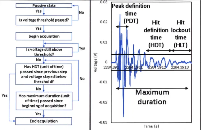
pre-amplifiers. Most AE systems have DAQs that operate on a hit-based architecture, meaning that only voltage pulses such as seen in Figure 2 are considered useful and thus recorded. The system logic as to what constitutes a hit and when a hit is terminated is specified in Figure 4. In normal operation summary statistics such as time, duration, amplitude and energy are recorded,

Pre-amplifiers Data acquisition system

PA5

-DAQ

PA7

but the actual voltages of the hit are not in order to save hard drive space. If the voltages of the hit are to be recorded, the analog-digital converter is used to digitize the hit. However, while the length of a hit is flexible under the analog system, the digitized voltage can only save for a specified number of samples that is independent of the actual hit length.

0.03

Passive state

Peak definition

Yes _No

time

I s voltage threshold passed? _{0.02 (PDT) Hit Hit}

Yes

_{definition lockout}

Begin acquisition _{tme tme}

0.01

Yes HDT) (HLT)

Isvoltages labove _e threshold?

No W

Has HDT (unit of time) 2284.39 1 284.3913

passed since previousstep

I

and voltage stayed below _No

threshol d? -0.01

No, _{Nol ~Maximum}

₁

Yes Has maximum duration (unit

of time) passed since _-0.02

duration

beginning of acquisition?

Yes I

-+ End acquisition -0.03

Time (s)

Figure 4 - (Left) AE DAQ system logic for determining a hit (Right) Illustration of HDT and maximum duration in the context of a waveform.

Peak definition time (PDT): the time over which the maximum amplitude can be defined for

an AE hit. The time begins counting upon trigger.

Hit definition time (HDT): the time during which the system waits for new incoming signals,

as illustrated in Figure 4.

Hit lockout time (HLT): the time after a hit during which no new acquisition can be started.

This is to prevent reflections from re-triggering the system.

Event: when an acoustic emission is generated in a specimen, hits are detected by multiple

sensors. Typically an acoustic emission event is inferred to have occurred when 4 or more sensors detect hits within a short window of time. This is illustrated in Figure 5. When viewed on a longer time scale in relation to parameters such as amplitude or energy, events tend to take the form of vertically clustered scatter points. This is because sensor receives a different amplitude, and the time between different sensors is very small relative to the time scale of the experiment. An example is shown in Figure 6.

0.05 -0

Sensor

1

Sensor

2

Sensor

3

-0.05

Sensor

4

Sensor

5

-0.05

Sensor

6

Sensor

7

Sensor

8

-0.05

Figure 5 - An example of an AE event: multiple hits are received in a short period of time on different sensors. The arrival time is shown in the circle. Sensors are laid out as in Figure 3.

.1;,

.

-~

I

Figure 6 - Amplitude over time for all sensors in a hydraulic fracturing experiment. Each scatter point represents a single hit. Events are defined as the occurrence of multiple related hits within a short period of time, which can be inferred to be the vertically clustered groups shown in the red lines. They are vertically clustered because each channel detects a different amplitude since the distance to the source varies.

Waveform: the digitized voltages of a hit is known as a waveform. It is sampled at regular time intervals for a fixed number of samples denoted as the waveform length. Waveforms are often, but not necessarily, recorded in conjunction with a hit. In seismology a waveform is referred to as a seismic trace.

Channel: relates to a sensor in the sensor array and its associated conditioning such as amplification or filtering 0-07 0. 0- 06-05 0-04 1 V

71-

I

I

Amplitude: a value representing the magnitude of a hit. This is often expressed in decibels (dB),

defined in Equation (1) below. Decibels in the context of AE are logarithmic, similar to sounds in human hearing range. The coefficient of 20 indicates that every increase of 20dB corresponds to

a iox increase in voltage. The reference value for dB in AE is 1 pV.

dB=2Oog

(

dB = 20 log m cto Ft = 20 log(V(ptV)) - Amplification Factor (dB) ()

(Amplification Factor

Where: dB is the amplitude in dB

V(pV) is the voltage in microvolts

Amplification Factor is the pre-amplifier factor where lox = 2odB, io0x = 4odB

and iooox = 6odB.

As an example, the hit in Figure 2 has a maximum voltage of o.2V at an amplification of 20dB

(1oX), so the amplitude of the hit in decibels is 20*log(O.2*10 6) - 20 = 86dB.

Duration: a parameter that is representative of the amount of time over which energy was

released in the specimen. Typically the length of a hit is taken to be the duration.

Sampling rate: the user-defined rate at which the digitizer samples hits for digital storage. The

analog system samples at a fixed 1oMHz. The recorded waveform in Figure 7 shows the relative scale of the sampling rate in the context of the frequency of the waveform.

0.01 0.008 0.0064 0.004 5 0.002 0 Z 2833301 2483,3301 1 8.3301 2483.3 248a.3 2483.33J2 >-0.002 -0.006 -0.008 -0.01 Time (S)

Figure 7 - Sample waveform showing the relative scale of AE sampling rate to the oscillation

frequency. Each point is a datapoint sampled at 5 MHz.

Attenuation: the decay in amplitude and frequency of a signal as it travels through a medium.

Energy: the strain energy of a hit can be found by taking the integral of the square of the

waveform as shown in Equation (2). Given that the voltage is used directly, the energy is in units

of V2_{s, and so must be calibrated to a known source to express the energy in terms of joules.}

E = fA2(t)dt (2)

Where: E is the energy of the waveform in V2s

A(t) is the amplitude in volts as a function of time

Kaiser effect: the phenomenon that few AE hits are observed until the historical maximum

stress experienced by a specimen is reached. This is analogous to the concept on a pre-consolidation pressure in soil mechanics.

Felicity effect: the phenomenon that the Kaiser effect does not hold for a material that

undergoes significant damage at its historical maximum stress. This can be expressed as the Felicity ratio f, where PA is the stress at which AE begin to generate, and P1 t is the historical

a material suffers from more damage, the Felicity ratio decreases. This has been used in concrete structures as an assessment of damage (Grosse and Ohtsu 2008).

Pressure wave (P-wave): Acoustic emissions generate both pressure and shear waves. The

pressure wave travels in the direction of propagation, and behaves similarly to a sound wave. Particles in a shear wave move perpendicular to the direction of propagation, similarly to ocean waves. The differences are illustrated in Figure 8. This work only considers P-waves, as the transducers used are sensitive to these waves.

Figure 8 - (Top) Illustration of P-wave. (Bottom) Illustration of S-wave. (Shearer 2009)

2.2 AE ANALYSIS TECHNIQUES

The following section describes some common methods of processing AE in order to produce meaningful results beyond the waveforms themselves, and their basic summary statics such as energy, amplitude, frequency and duration. The two main methods of analysis are: a) the inference of the location of the source of an AE event based on the pattern of its arrival times and b) the classification of the events based on data processing of the waveforms that make up an event. Section 1 outlines the process of localization, while sections 2.2.2and 2.2.3 outline classification techniques.

2.2.1. Localisation

Localization is the process of inferring the location and origin time of an acoustic emission given a set of arrival times detected by the sensor array. This is schematically represented in Figure 9, where an acoustic emission is emitted and each sensor detects a waveform after some ti. The difference between arrival times of different sensors can then be used to predict the location of the source. 4

Source

S4

S5

S3

S6

S2

S7

S1

Figure 9 - Schematic of the travel time associated with a source at the centre of the specimen and an 8

sensor array. The travel times can then be used to infer the location of the source.

The first step in this process is to accurately determine arrival times for each channel. The main issue in this regard is the uncertainty associated with defining the arrival time, as illustrated in Figure 10 which shows the first segment of a recorded waveform.

I

* 10-3 -2 Threshold 8 --10 -12--14 1842,2836 1842 2836 1842 2836 1842.2836 1842,2836 1842.2 8422836 2836 18422836 18422836 Time (s) [

Figure 10 - Sample waveform arrival. Waveform segment that initially shows background noise, followed by the onset of an acoustic emission. Data points shown in circles. The arrival time is most likely to be the time shown at A, but can also be estimated using a threshold (red line), resulting in the arrival time estimate B. The difference between A and B is illustrated in green.

Intuitively, the first arrival of the waveform is likeliest to be at the time labelled A, which is the first time the voltage diverges significantly from zero. In order to reliably find this point, there exist several methods. The simplest method is to assign a threshold voltage value (red line), and to denote the time at which the waveform exceeds this value as the arrival time (Label B). Although the arrival time is not correct, it is expected that the curvature of the first arrival (green segment) is similar for all sensors and so the offset between the true arrival time and the threshold arrival time (i.e. tB-tA) is roughly constant. As a result, the difference in arrival times between sensors

would still be correct and the calculated source location should still be accurate. This is described schematically in Figure ii, which shows that the slope in the distance-time space should be similar between the thresholded arrival time and the true arrival time. Another limitation is that the

threshold is a constant value while the amplitude of waveforms change over time. The thresholded arrival time is used for the majority of the work presented in this thesis, although further work will attempt to use more sophisticated methods to find the true arrival time.

-Time

Sensor 1

Sensor 2

Sensor 3

-Sensor 4

Distance from source

Constant offset

Figure 11 - Schematic of the waveforms observed by 4 sensors located at an increasing distance from

the source. The arrival times estimated from a threshold are shown in red, and the true arrival times shown in blue. It can be seen that ideally there is a constant offset between the true arrival and the thresholded arrival such that the origin time is incorrect but the inferred source location is correct.

One such method is the Akaike Information Criterion (AIC) (Akaike 1974) which is presented in Equation (3).

AIC(tw) = (tw - to) - log(var(Rw(to, tw))) + (Tw - twe+) -1og(var((Rw(tw+1, Tw)))

Where:

(3)

w is each data point of the waveform

tw is the time at data point w

to is the time at the start of the waveform

Tw is the time of the last data point

var(Rw(tw+1,T.)) is the variance of all the voltages from tw+1 to Tw

The method works as follows: a window of time containing the arrival is taken, such as in Figure

12. For each data point w, Equation (3) is applied to find an AIC value for that point. The result is

the blue line in Figure 12, which has the same time scale as the waveform (orange). The AIC value

initially decreases because if it is assumed that the initial portion of the curve consists only of background noise, then the first term in the AIC equation decreases with increasing time since the sample size increases while the sample variance is constant. However, as soon as any perturbations from the arrival signal occurs, the sample variance increases due to the AE signal deviating significantly from the background noise. As a result, the first term of the AIC equation increases as soon as perturbations occur, leaving the minimum value AIC value as the last point in time before perturbations occur. This corresponds to the arrival time of the AE signal. For most applications the second term in the AIC equation has less effect than the first term since the variance of the AE signal is very high.

0 Minimum AIC -0 j VV 338 8478 3388478 338 8478 338 8478 338 8478 338 8478 3388478 338 8478 338-8478 338 8479 Time(s)

Figure 12- Illustration of AIC. Orange line shows the initial portion of a recorded waveform. The AIC values for this waveform are shown in blue. The time corresponding to minimum AIC is set to be equivalent to the arrival time.

In terms of the actual localization, there have been analytical solutions proposed based on inverting the arrival times (Hardy 2003), where it is assumed that

di = vi (ti - to) (4)

Where di is the distance between the source and sensor

vi is the velocity

ti is the arrival time

to is the origin time

This equation is expressed for each sensor, from which a matrix can be constructed and solved for di and to. However, the lack of an error term in the equation leads to numerical instabilities if there is variability in the arrival times. Most techniques used today are variations of an error minimization function. The basic premise is that for a sensor array and its corresponding arrival times, it is possible to calculate a residual for any location (Grosse and Ohtsu 2008). The residual can then be found for all likely locations of the source (search points), and the location with the lowest residual is likeliest to be the true source location. The most common forms of the residual function are given in Equations (5) and (6).

n -- 2 (5)

1 (^ - X,)2 + (y,y)2

Residual (L2) = t( Y

Residual (L1) = tX-)2 + ,-Y)2

(6)

and

y

xi, yi and ti are the x co-ordinate, y co-ordinate and arrival time for each sensor i respectively.

L1 is the absolute of the residual, whereas L2 is the square of the residual and is more sensitive to

outlying data points. As a result, L1 is generally used since sensors far from the source can have

large errors due to signal attenuation. An example of the spatial distribution of L1 and L2 residuals

is given in Figure 13. The origin time can then be calculated by back-calculating the travel time for each sensor at the optimum location and taking the average, as expressed in Equation (7).

E=₁

ti

Figure 13 - Residual values for the arrival times given in Figure 5. Left side shows Li residuals, right

side shows L2 residuals. The location corresponding to minimum residuals is the likeliest location to be the true source location.

The accuracy of this technique can be improved by implementing an algorithm that removes channels with erroneous arrival times from the calculation. This can be done by determining whether any channels have a significantly higher residual than the other channels, and then re-calculating the residuals without the erroneous channels.

In terms of improving the speed of this technique, the main improvement would be to implement a search algorithm such as the downhill simplex to find the minimum residual without calculating the value for each point on the grid. This will be implemented in further work.

The relative difference modification (Shearer 2009) to the traditional localization approach is a useful technique where the events to be located are within close proximity. The basic principle is still to consider a number of search points, calculate the residual at each, and denote the search point with the lowest residual as the true source location. The difference lies in the calculation of the residual. In addition to calculating the difference between the search point and the sensor, it also calculates the difference between a chosen master event and the sensor location. By referencing localization to this master event, it is possible to account for the variations in the velocity field since the velocity field affects both the master event and the grid point equally. By subtracting the error of the master event from the error of the search point, the effect of the velocity field is reduced. The concept is illustrated in Figure 14.

ti

Grid

search point

Residual based on

tmi

arrival times

Located at (x,y)

Master event

Sensor

(xi yi)

Figure 14 - Illustration of double difference method. Schematic showing the location of the master

event, the grid search point, and the sensor. The grid search point ti is compared to the master location

xm, ym for both the observed arrival times and the calculated arrival times.

The best form of a master event is one where the location is known, for example an artificial source such as a pencil lead break test. However, the pencil lead break can only be performed at the beginning of an experiment, whereas much of the damage affecting the velocity field occurs close to failure. As a result, for events close to failure it may be more accurate to use a large amplitude event as the master. To calculate the likeliest location using the relative difference technique, the residual is modified as follows:

[ X,)2 + y)2 _I(X X,)2 + (ym - y,)2 2

Residual (L2) = (ti - tmi) - -

(

Residual (L₁) = (ti - ti) - v Y i))9)

Where tmi is the arrival time of the master event at sensor i

xm, ym are the x and y co-ordinates of the master event

The terms are also depicted in Figure 14.

These equations take the same form as Equations (5) and (6), but the observed arrival time t is replaced by the term (ti - tmi) which is the difference between the observed arrival time and the

observed arrival time of the master event. Likewise, the predicted arrival time is

replaced by - "(XXi)2

+m- , which is the difference between the predicted

V V

arrival time of the search point and predicted arrival time of the master event. In this way the errors due to the velocity field are mitigated since the velocity field affects the ti term and the - _{term equally, such that the resultant residual does not contain the influence of the} velocity field.

2.2.2.Source characterisation - Moment tensor

The oscillations seen at the transducers originate from a release of energy within the rock specimen. This can be expressed as:

Uk(X, t) = Gkp,q (X, Y, t) * S(t)Cpqijfn liAV (10)

Where Uk (X, t) is the displacement at location x, time t and direction k which is the displacement seen at the sensors.

Gkp,q (X-, Y, t) is the spatial derivative of the Green's function describing the displacement at location x and time t given a point force y. This component

describes the geometry as well as material properties pertaining to wave propagation.

S(t) describes the kinetics of the source i.e. the amplitude of energy release over time, as illustrated in Figure 16. Cpqij is the elastic tensor such that i =

Gkp,q(X,9, t)Cpqij

nj is the normal to the crack plane

lj is the direction of crack motion. This is illustrated in Figure 15

AV is the crack volume.

n.

n.= I.

_I,

n.

Ii

Figure 15 - Schematic transverse view of a crack showing normal and crack motion vectors for a) a

shear crack, b) a tensile crack, c) a mixed mode crack

Conventionally, the moment tensor is defined as follows:

Mpq = CpqijnjliAV (I1)

And is known as the "moment" tensor since it has units N .m3 = [Nm]. This tensor describes the

stress-strain properties, directionality as well as size of the source, and is thus considered to be the most complete representation of the source mechanism.

0.0 3.17 6.35

Time (xlO 6s)

Figure 16 - _{Example of a source-time function S(t) (solid line) of an acoustic emission as compared to}

a synthesized function (dashed line). It can be seen that an acoustic emission increase quickly from o to maximum energy output, and maintains a residual energy output for some period of time. (Grosse and Ohtsu 2008)

For an isotropic medium, the elastic constants are known and so the elastic tensor can be multiplied by the normal vector and the direction vector to give:

)Akk + 2p11n1 V(11 2 + 12n) p(11n3 + 1₃ni)

Mpq = jiln2 + 1₂nj) Alknk + 2.11₂n2 P02n3 + 13n2) AV

po1n + 13nj) (12n3 + 13n2) )dknk + 2913n3 (12)

Where p and X are the Lame parameters. This tensor is analogous to the stress tensor in that the diagonal components correspond to normal components that cause volume change, and the off-diagonal components to shear behavior such as a shear crack. This is illustrated in Figure 17.

Figure 17 - Moment tensor components given a unit cube (solid line). An exaggerated view of the deformed cube is shown in the dashed lines.

In order to solve the inverse problem of finding the moment tensor given a set of displacements at sensor locations, the Green's function is required. However, the function can only be fully

solved analytically for an infinite space or for the far field, and so known solutions in a half space are compared with the infinite space and far field solutions. If the far field is assumed, Equation (1o) can be simplified as shown in Equation (13) below.

1 ri dS(t)

Ui )= -~r rqMpq dt(13)

UKl =4lupvp R _dt

Where Ui (-x, t) is the displacement at location K and time t

p is the material density

Vp is the P-wave velocity

ri is the derivative of the Green's function

rp is the vector between the source and location K

M33 --- _{---- --- 7%%} K" M23 IL \--M3 M 3 M 9121 M32 M M22 Ii

rq is the transpose of rp

R is the distance between the source and location 3

Mpq is the moment tensor

is the time derivative of the energy source function

Given that most AE are not collected in the far field or in an infinite space, a correction is needed to relate boundary conditions for a typical experiment to the far field. It was found that the amplitude of a first motion in a half space is related to the first motion amplitude in an infinite space or the far field by a reflection coefficient:

Where R (t r) = 2k 2_a(k2 -2([1 - a2_]) (14) e , _(k2 _{- 2[1 - a}2 ₂ ])2 _{+ 4a[1 - a}2 _/k2 _{- 1 + a}2

f

i is the vector between the source and the sensor (See Figure 18)

k=V,/Vs

a= r-f

Sensor

Figure 18 - Schematic of a source in relation to the sensor. t is the normal vector of the sensor, and r

is the vector between the sensor and the source.

t

r

It is assumed that for most experiments where the sensor is at a specimen boundary the half-space assumption holds true. As a result, the first motion amplitudes seen in experiments can be related to the far field solution by the reflection coefficient Re. For the case where t is parallel to r, Re = 2, implying that a P-wave travelling directly to the sensor face produces a first motion amplitude that is double that it would have been in an infinite space or in the far field.

Given that the voltages observed by the sensors are not directly related to the displacement at that location and that the Green's function is approximated for an elastic half space, Equation (13)

cannot be used to derive the true values of the moment tensor without calibration. Consequently, the results are generally used comparatively between events within a similar experimental setup, or used only for the directionality of crack motion. As a result, the constants in Equation (13) can

be removed, and it is also assumed that dS(t) = 1 given that only the first motion is used and so the energy function over time is not used. Finally, the amplitude of the first motion is simplified

and expressed in Equation (15) below.

Re6 f)

A() = Cs R' rprq Mpq (15)

Where A(x) is the first motion amplitude at sensor location x

Re(, f) is given above

rp is the vector between the source and location i

rq is the transpose of rp such that rprq Mpq is a scalar

R is the distance between the sensor and the event

Mpq is the moment tensor as defined above

Cs is the bonding coefficient for each sensor, and can be found by inducing a known reproducible event such as a pencil lead break and applying A()= (C) for each

sensor. The rprqMpq term is not considered since a pencil lead break is a point force and not a crack.

In full matrix form the equation can be expressed as:

Re([) 1 1 Mi 1 2 M 1 3

i

A(x) = C s r2 t, [r1 r2 r3] M1 2 M 2 2 M23 r2 rm_{1 3} M2 3 M3 3 r3

This equation can be expressed for all sensors within a sensor array, forming a system of n equations with 6 unknowns. As a result, at least 6 sensors are required for 3D moment tensor decomposition. This solution of the moment tensor is known as SiGMA (Simplified Green's function for Moment Tensor Analysis) and is suitable for the current experiments since it is relatively robust, computationally simple and the parameters are easy to obtain.

Various summary statistics can be found from the moment tensor components calculated using Equation (15). The ratios denoted as X, Y and Z are one such set of statistics. Physically, they represent the contribution of the off diagonal elements, the deviatoric of diagonal elements, and the uniform diagonal elements of the moment tensor respectively. For example:

M1 1 m12 M1 3 0 0 1

M1 2 M2 2 M23

=10

M1 3 M2 3 M3 3 1 0 0

[Mn

M1 2 M2 2 m23 0= 1 0] would have X=o, Y=o, Z=1

IM1 3 M2 3 M3 3 0 0 1

F

M1 2 M2 2 M2 3 =10 -1 01 would have X=o, Y=1 and Z=o.

M1 3 M2 3 M3 3 0 0 2

X: Represents shear Y: Represents deviatoric Z: Represents uniform

of normal stress normal stress

Figure 19 - Physical representation of ratios X, Y, Z. X represents the off-diagonal shear components

of the moment tensor, Y represents the deviatoric of the diagonal elements, and Z represents the

uniform component of the diagonal elements. (Grosse and Ohtsu 2008)

These ratios can be calculated from the eigenvalues of the moment tensor, as expressed in

Equation (16). 1 = X + Y + Z (16) e2 ₁ -= o--Y+Z el 2 e3 1 -= -X--Y+ Z el 2 Where eigenvalues ei e2 2 e3

-The shear contribution ratio X, which represents the off-diagonal elements of the moment tensor, is dominant for sources that have shearing motion. Similarly, a uniformly expansive source would be mostly isotropic, and so the ratio Z would be dominant. For a source such as a tensile crack, only one of mn, m2 2 or M33will be dominant, and so the ratio Y, which represents the deviatoric

of the diagonal elements, will be the largest. The X, Y, Z ratios are illustrated in Figure 20. Since the primary source types of interest are shear and tensile cracks, the main distinction is whether the shear ratio X, or the deviatoric ratio Y has the largest contribution. It is generally assumed that the ratio Z is small for cracking behavior. By convention it is considered that events with X <

40% are tensile, those with X > 6o% are shear, and those in between are of a mixed mode.

However, this convention is largely defined for cases of uniaxial compression, whereas the hydraulic fracturing experiments in this thesis present a different loading condition. As a result, it may be useful to also consider the Z ratio, given that the water pressure may act uniformly upon crack surfaces.

Figure 20 - Schematic of a penny shaped crack (black) with deviatoric tensile (red), shear (green), and

uniformly expansive (blue) stresses acting upon it.

The crack normal vector i- and crack motion vector

I

(17)

For a tensile crack, the normal vector f and the motion vector ii are parallel, and so T7 is coincident with the opening direction since I + ii = 21= 2-n. For a shear crack, eland 63 can be used to derive the normal and motion vectors where ii = " and i = T+3

2 2

However, recall that Mpq = CpqijnjliAV, where AV is a constant. It can be seen that n and 1 are multiplied by the stiffness matrix in the same way, and so they are numerically indistinguishable given Mpq without having an external piece of data. As a result, the n and 1 obtained above could easily be 1 and n instead. For tensile cracks this is not an issue since the two vectors are co-linear, but for shear cracks n and 1 are indistinguishable. However, with comparison to the high speed and high resolution images it may be possible to see the direction of crack motion or the crack orientation for some events. The AE corresponding to that crack can be found, and SiGMA applied to find the two supposed 1 and n vectors. The calculated vector that best matches observations from the photos can then be used to separate 1 from n; this calibration can then be applied to all events. A hypothetical example is given in Figure 21.

B

A

Figure 21 - Experimental crack geometry showing a hypothetical shear event (green) and a

linear, so there is no ambiguity in the crack orientation. For the shear event, fi and I are not co-linear, and so two vectors are output from the moment tensor code but cannot be distinguished from each other without additional data. The visually observed crack geometry provides this information,

for example in the schematic above it is clear that the vertical vector is I, and the horizontal vector is

in.

In some cases, ii and i can form an obtuse angle to each other, resulting in the ratio X exceeding 1 or being less than o. In this case the angle c between ii and ! can be found using X =

(1-2v)-(1-2u)cosc

(1-2u)+cosC , readjusted to the corresponding acute angle, and the X, Y and Z ratios

recalculated.

The above derivations are for a 3D case, but the experiments in this thesis are mostly in close to a plane stress condition and the sensors were also mostly located in the same plane. As a result, it is realistic to make a simplifying assumption that the AE waves observed only travel in the x-y plane, as illustrated in Figure 22.

Z

Y

Specimen

Source

Sensor

Figure 22 - _{Schematic showing plane waves travelling in a specimen whose depth dimension is}

relatively small compared to the other 2 _{dimensions. It can be assumed that the sensor receives}

The inherent assumption is that the cracks are coplanar with the z axis, which is set to be equivalent to the M33 axis, and 1 and n assumed to have no z components. The moment tensor can

then be re-written as:

Xlknk + 2p[dnj ii(11n2 + 12nj) 0

Mpq = (ln₂ + 12nj) Xlknk + 2[l2n2 0 AV (18)

0 0 ?Llknk

Re-arranging the M33 term above using elastic relations gives the statement M3 3 = v(m11 + M2 2

)-Since only x and y components of the moment tensor are then required, Equation (15) can then be simplified as:

Re(tUi) rma 1 (9

A(x) = CsRe 62||[r, r2] M1 M12] [r1j (9)

11r1 r211 LrM12 in2 2] r2

Since it is assumed that r3 = o. The full 3D moment tensor can then be reconstructed as:

Mpq = M12 M2 2 0 (20)

0 0 V(M11 +

M22)-And the analyses methods given above for the 3D case can be applied.

2.2.3.Source characterisation - Polarity method

The SiGMA moment tensor technique provides insights into the nature of the microseismic events, where the output is the full moment tensor that describes the directionality of cracking as well as the tensor breakdown of the source mechanism. The method requires two pieces of information from each signal: the arrival time for localization, and the maximum amplitude of the first peak for the system of equations. From the experiments described in this thesis it appears that arrival times can be highly susceptible to error, and so a simplified event classification scheme known as the polarity method can also be used for comparative purposes. This method only requires the sign of the first peak motion, and outputs the classification of the crack type but gives no information on directionality. The method uses the assumption that a purely tensile event will produce motion towards all the sensors. Likewise, a movement of two grains towards each other

will produce motion away from all sensors, and a shear or mixed mode event will produce different first motions based on sensor location. This is illustrated in Figure 23 below.

Figure 23 -Illustration of polarity technique. A collapse (compressive) type event is shown on the left, tensile in the middle and a shear on the right. The expected polarity is shown for sensors located at the blue rectangles in each case.

The overall polarity of an event is taken to be the average first arrival sign of all the detected

waveforms, as stated in Equation (21).

n

pol = sign(A) (21)

i=1

Events with a polarity greater than 0.25 are considered compressive, events with polarity less than

-0.25 are considered tensile, and those with polarity in between are considered shear.

This method has been shown to be relatively similar to classification by moment tensor inversion

(Graham, et al. 2010), and so can be used by itself when only classification is required, or provides

a way to verify results from moment tensor analyses.

2-3 PREVIOUS EXPERIMENTAL WORK

One of the seminal papers in acoustic emissions applied to rock mechanics is by (Lockner, et al.

1991). In this experiment, a cylindrical specimen of Westerly granite was triaxially loaded with

AE hit rate remained constant. As a result, the material failed quasi-statically over the course of

5.5 hours. The stress-displacement curve is shown in Figure 24.

600 4-WjV 7Z 400 2 00 or I 2

Axial Shorteninig (mm)

Figure 24 - Stress-displacement curve of (Lockner, et al. 1991). Segments a-f refer to Figure 25

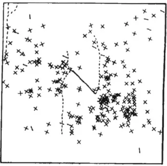
Under the AE rate control where the AE hit rate is kept constant, it was possible to observe the development of the failure plane shown in Figure 25. The localization of events has good accuracy, and the concentration of events noticeably changes from a diffuse nature (Figure 25) in the increasing portion of the stress-strain curve prior to failure (segment a, Figure 24) to a highly localized zone in segments b to f. It can be seen that the failure plane initiates at the peak stress (segment b, Figure 24) and is fully formed by the end of the stress drop in segment f. This localization of the crack plane as it grows would not have been possible given a load or strain controlled experiment since the load drops occurs very quickly in both cases and the individual events seen in Figure 25 would all be occurring in the time span of a few AE hits.

- lb C

a

-d

e

-8j

-!s *.. 1* -I d e (

4/

I

Figure 25 - Localisation of AE events at different stages of the experiment showing development of the

failure plane in (Lockner, et al. 1991). a-f refer to stages in the stress strain curve in Figure 24. The top

subfigures are viewed along strike and the bottom subfigures viewed face on.

The experiment also calculated the energy of hits localized in five different 1 cm3 cubes and plotted the cumulative energy output for each location over time, as seen in Figure 26. The authors estimate that locations Ci and C2 experience mode III failure from the development of the failure plane, and it can be seen that these 2 locations release energy over a longer period of time

compared to zones C3 and C4, which the authors postulate experience a 3:1 ratio of mode II to mode III failure. Co, which is located at the fault nucleation zone, releases a significant amount of energy at crack initiation but not much afterward since the crack can grow outwards. It can be seen that the curves for C1 to C4 have a step like shape, which the authors hypothesize may be due to heterogeneity in that there exist higher strength zones that temporarily inhibit crack propagation.

Along strike

Face on