Activity Recognition for a Smartphone and
Web-Based Human Mobility Sensing System
The MIT Faculty has made this article openly available.
Please share
how this access benefits you. Your story matters.
Citation
Kim, Youngsung et al. “Activity Recognition for a Smartphone and
Web-Based Human Mobility Sensing System.” IEEE Intelligent
Systems 33, 4 (July 2018): 5–23 © 2018 IEEE
As Published
http://dx.doi.org/10.1109/MIS.2018.043741317
Publisher
Institute of Electrical and Electronics Engineers (IEEE)
Version
Original manuscript
Citable link
http://hdl.handle.net/1721.1/120294
Terms of Use
Creative Commons Attribution-Noncommercial-Share Alike
Activity recognition for a smartphone and web based
travel survey
Youngsung Kim
Singapore-MIT Alliance forResearch and Technology (SMART)
[email protected]
Francisco C. Pereira
Singapore-MIT Alliance forResearch and Technology (SMART)
[email protected]
Fang Zhao
Singapore-MIT Alliance forResearch and Technology (SMART)
[email protected]
Ajinkya Ghorpade
Singapore-MIT Alliance for Research and Technology
(SMART)
[email protected]
P. Christopher Zegras
Massachusetts Institute of Technology (MIT)[email protected]
Moshe Ben-Akiva
Massachusetts Institute of Technology (MIT)[email protected]
ABSTRACT
In transport modeling and prediction, trip purposes play an important role since mobility choices (e.g. modes, routes, departure times) are made in order to carry out specific activities. Activity based models, which have been gain-ing popularity in recent years, are built from a large num-ber of observed trips and their purposes. However, data acquired through traditional interview-based travel surveys lack the accuracy and quantity required by such models. Smartphones and interactive web interfaces have emerged as an attractive alternative to conventional travel surveys. A smartphone-based travel survey, Future Mobility Survey (FMS), was developed and field-tested in Singapore and col-lected travel data from more than 1000 participants for mul-tiple days. To provide a more intelligent interface, infer-ring the activities of a user at a certain location is a crucial challenge. This paper presents a learning model that in-fers the most likely activity associated to a certain visited place. The data collected in FMS contain errors or noise due to various reasons, so a robust approach via ensemble learning is used to improve generalization performance. Our model takes advantage of cross-user historical data as well as user-specific information, including socio-demographics. Our empirical results using FMS data demonstrate that the proposed method contributes significantly to our travel sur-vey application.
General Terms
Algorithms, Design, Human Factors, Experimentation
Keywords
Activity Recognition, Urban Mobility, Interactive Data Col-lection.
1.
INTRODUCTION
Human activity recognition research is useful to interpret mobility related phenomena in a city [21]. Understanding why people go to some places at certain times has beneficial ramifications in many fields such as transportation, internet commerce, urban traffic management, location based ser-vices, public health, urban planning, public safety, and so on [17]. Activity based modeling for travel demand is gain-ing popularity in recent years and it requires a large number of observed trips and their purposes to build. Traditionally, data used in activity based modeling is collected through interview-based travel surveys. Collecting a sufficiently large sample requires an extensive effort. The accuracy of the col-lected data depends on the memory of the participant, so it is a challenge to capture high resolution activities for days with complex activity patterns. Due to these limitations, re-searchers are exploring new ways to conduct travel surveys using mobile sensing devices. Smartphones are pervasive devices that nowadays people carry with them everywhere. They are ideal devices for travel and activity information logging. We have developed a smartphone based activity-travel survey system, Future Mobility Survey (FMS) [3], and recently used it in large-scale data collection effort in Singapore.
FMS acquires movement data through sensors (such as GPS, GSM, WiFi, and Accelerometer) commonly available in current smartphones. Besides the hardware sensors, FMS acquires activity and transportation information through a web-based interactive process. The task of the participant is to check that the stop locations, activities, times, and modes are accurately described (and correct them if nec-essary) on a web interface. To ensure quality of validated data, the user must accurately label the activity at each stop location. Machine learning based approaches for ac-tivity recognition can automate some of these tasks, reduce user burden, and therefore assist the user in providing much needed high quality data. Currently a new version of FMS
software is being developed based on data acquired during a field-test to create a more intelligent backend and inter-face. In this paper, we present a learning based model for the activity recognition task.
However, prediction of human activity is a nontrivial task, especially in an urban area. One of the reasons is that activ-ities often have heterogeneous patterns within a small area (e.g. shopping malls with healthcare facility, supermarket, offices) or at the same time (e.g. working at home; shop-ping while waiting for the train). Also, sensor data quality itself is not always the best (e.g. GPS unavailable in indoor activities).
To alleviate uncertainty of real world data, we extract het-erogeneous features and merge multiple hypothesis models learned from different user populations. The user’s likeli-hood of performing a certain activity at a given location will depend on user’s personal needs which will be driven by his/her socio-demographic characteristics [13]. Usually en-vironmental context at the given location limits the type of activities one can perform. We can also derive the activity likelihood from the activities performed by general popula-tion apart from individual user characteristics. In this pa-per, we present a learning model based on spatial, temporal, and contextual features and conduct various experiments to demonstrate its veracity. The contributions of this paper are:
• A method to generate a set of predictive features based on location, time, transition context, and environment context (e.g. Points of Interest),
• Spatial data quantization methods to balance the noise effect in real world data,
• Improvement of generalization performance by merg-ing of intra-user data and inter-user data includmerg-ing user’s social-demographic information,
• Analysis of number of training days required for a learning model in a real world application.
This paper is organized as follows. In section 2, we re-view related work. In section 3, we present FMS, a smart-phone based activity-travel survey where the proposed ac-tivity recognition algorithm will be used. In section 4, we present the proposed activity recognition framework. Ex-tensive experiments are followed with different settings of feature in section 5. Finally, we conclude this paper with some remarks and future work in section 6.
2.
RELATED WORK
With the advance of sensing technology, GPS loggers, and more recently, smartphones, have become popular tools to conduct travel surveys that are essential for transportation planning and management [2, 3]. The identification of ac-tivities is perhaps the most challenging data processing task involved in such travel surveys. The activity categories typ-ically include home, work, social, shopping, pickup/drop-off etc.
Most of the algorithms used to derive activities in GPS travel surveys are rule-based and rely heavily on GIS in-formation, such as Point Of Interest (POI) and land use information [23, 8, 6]. An early car-based study in America
by Wolf et al. [23] inferred trip purposes from GPS data and an extensive GIS land use database. In more recent work, POI’s attractiveness is defined along time of day to indi-cate the potential possibilities for activities [8], and [6] pro-posed to infer an activity based on the distance between POI and the stop location. Another option is to use individual characteristics as input for activity recognition algorithms. Axhausen et al [1] developed a rule based approach to iden-tify activities based on users’ home and work locations, and POI/land use information in the Swiss. Similar information and rules were used in the GPS survey in the Netherlands [2]. Reference [22] described a more complicated heuristic rule-based method which collects users’ workplace or school, the two most frequently used grocery stores, and occupation beforehand to be used to derive trip characteristics.
More elaborate algorithms have been proposed taking a machine learning approach. Deng and Li [4] used attributes such as land use, sociodemographic information of the re-spondents, etc. to construct decision trees. An adaptive boosting technique was used to improve the classification results. Liao et al. [15] proposed a location based activ-ity recognition system using Relational Markov Networks. These works are evaluated based on small samples of exper-imental data.
Few work exists for activity detection in smartphone based travel surveys. Feldman et al. [5] converted GPS trajecto-ries collected by smartphones into lists of activities by first finding businesses around a user stop, and then employing reverse Latent Semantic Analysis (LSA) to look up the most relevant terms associated with the businesses.
3.
SMARTPHONE-BASED ACTIVITY TRAVEL
SURVEY
In this section, we give an overview of the FMS system and briefly describe the data which is used for building activity recognition algorithm.
3.1
Future Mobility Survey (FMS):
activity-travel data collection method
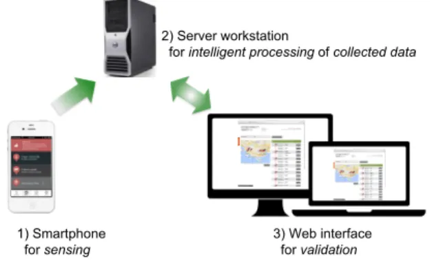
Future Mobility Survey (FMS) [3] collects mobility records through a smartphone application (Android and iOS) and an interactive web interface. It acquires movement data through sensors commonly available in current smartphones, namely Global Positioning System (GPS), WiFi, Mobile Com-munications System (GSM, CDMA, and UMTS), and Ac-celerometer. Stop and mode detection algorithms are run in the backend on the collected raw data and the output is presented to the user in the form of an activity diary [18, 3]. users can then “validate” their data by confirming or correct-ing the system generated stops/modes. In the current FMS system, there is a simple rule-based algorithm to detect only “home”, “work”, and “change-mode” activities. The overall flow is depicted in Figure 1.
FMS was recently deployed in Singapore [18] to conduct a travel survey. Thus far, the FMS has collected collected a total of 22,170 days from 1,440 users in real life situa-tions (more than 130 Million GPS points in total). Among the days and users, we have a total of 7,856 validated days from 948 users. A total of 793 users fully participated in this venture, each one required to collect data for at least 14 days and validate least 5 days. The survey was conducted between October 2012 and September 2013. Due to
bat-tery limitations, the smartphone application cannot contin-uously collect the high quality data (e.g. high accuracy GPS and big frequency accelerometer), and as a consequence, the records are sparse in practice. Furthermore, some sensors are not available in certain contexts (e.g. GPS unavailable indoors, WiFi unavailable without nearby APs).
1) Smartphone for sensing
2) Server workstation
for intelligent processing of collected data
3) Web interface for validation
Figure 1: Overview of Future Mobility Survey
sys-tem. The FMS web interface can be found at
http://www.fmsurvey.sg/.
To our knowledge, FMS is the only smartphone based travel survey that has gone through a field-test with large number of users. Most existing applications [8, 6, 15, 5] have used limited size of data collected by fewer than 28 users. The large amount of real world data collected presents a unique opportunity to develop and test machine learning algorithms for activity recognition.
3.2
Activity categories
Within the FMS, we have defined seventeen different ac-tivities. Home, Work, Work-Related Business, Education, Change Mode/Transfer, Pick Up/Drop Off, Meal/Eating Break, Shopping, Personal Errand/Task, Medical/Dental (Self), Social, To Accompany Someone, Recreation, Entertainment, Sports/Exercise, Other’s Home, and Other. ‘Other’ will be excluded in our activity recognition algorithm.
4.
METHODOLOGY
In this section, we first present a spatial quantization tech-nique to get empirical activity probability based features. We then describe the ensemble learning based classification methodology using heterogeneous features for different user populations.
4.1
Spatial-temporal data representation and
quantization
4.1.1
Data representation
Our dataset consists of a sequence of n stop points for a user u, {pu
i|i = 1, 2, . . . , n, and u = 1, 2, . . . , U }, where the
user stayed for a relevant time window1. Further each stop point is represented as pui = (xi, yi, ti1, ti2), where xi and
yidenote the geographical coordinates, (ti1, ti2) denotes the
start and end time respectively. For simplicity, we use pi
instead of pui now on. 1
The FMS minimum threshold is 1 minute to capture mode changes, but it is normally aggregated (by the system or by the user) to much longer chunks.
4.1.2
Data quantization
The quantization is applied to the location and time space to enhance data interpretation in terms of context. This context is coarse-grained in spatial and temporal axes. For example, we can deduce a “transportation change mode” during “evening rush hour” or deduce that a person may be at “shopping mall” on “Sunday evening”. Here, we ap-ply quantization as follows (where 7→ represents a mapping relationship):
• Spatial cell: the location (xi, yi) 7→ a cell ci.
Distri-bution of activities is non-uniform across geographies. Dependent on a mapping function, samples in a cell are different. Some spatial quantization methods will be proposed in section 4.1.3.
• Set of time slots (within the day): the time period (ti1, ti2) 7→ a set Siof time slots (e.g. 10 minute slots).
For example, an activity started at 8:53 and ending at 9:08 will be assigned to a time slot set S={8:50, 9:00, 9:10}. This works as an “temporal alignment” step that will later be useful for calculating temporal frequency features.
Hence, our dataset will consist of activity points qi (the
quantized version of pi), defined as the tuple (ci, Si, ai) where
aidenotes an activity from the set of sixteen categories
men-tioned above. We also create two useful functions: W(s) returns the day type of a time slot s (weekend or weekday); X (c) retrieves the set of Points of Interest from our database, corresponding to cell c.
4.1.3
Spatial quantization methods (distribution
adap-tive quantization)
As mentioned above, the function mapping the location of pito a cell ciaffects the likeliness of activity aiso we
ex-plore different mapping (spatial quantization) functions to find an appropriate population representation. The simplest and easiest way is to divide space arbitrarily regardless of a sample distribution. An adaptive way is to apply the data distribution. In this work, we consider both fixed quanti-zation and dynamic quantiquanti-zation. In the fixed case, once space of training data is quantized, it is used in future prob-ability calculations. In the dynamic case, space is divided when a new instance is identified. In this case, if there are N samples to calculate frequencies, the number of cells is N .
Fixed cell.
• Rectangle shape: quantization is not correlated with regional distribution. The easiest way is to adopt a rectangle shape; parameters including width (horizon-tal) and height (vertical) size.
• Voronoi tessellation based polygon: spatial data clus-ters can be found to apply regional characteristics. Based on a centroid of each cluster, edges and ver-tices of each cell can be found by Voronoi tessellation. To find an appropriate cluster is a essential process.
Dynamic (instance based) cell.
• Circular polygon: a cell is defined within predefined distance (radius of circle) at each instance. Every in-stance is a centroid of a cell.
4.2
Proposed features
4.2.1
Activity Frequency
For each activity point qi, we determine three kinds of
activity frequency: Temporal activity frequency, Spatial ac-tivity frequency, and Contextual acac-tivity frequency. We es-sentially make use of the following general empirical condi-tional probability distribution (we use the kronecker delta notation, where δi,j= 1 if i = j, and 0 otherwise):
P r(ai= l|bi) := PN j=1δaj,l· δbj,bi PL l=1 PN j=1δaj,l· δbj,bi (1) where N denotes the total number of activity points in the same cell for all users u ∈ U (U is a user set), bi denotes
a bin, and l denotes an activity type (L is total number of activities).
In this equation, we count a normalized frequency of activity l, within a bin over the total count of all activities within the same bin. For spatial activity frequency, the bin we use is a spatial cell ci.
In order to estimate the temporal activity frequency, we need a slightly more sophisticated treatment of the data. In this case, the statistics depend on the time slot sequence of the activity points, where each time slot adds 1 (e.g. an activity that spans from 8:00 to 10:00 contributes 12 to the total count, assuming 10 minutes time slots). The bin at activity point i is now defined by its entire sequence of time slots (Si). Inclusion or exclusion of a different activity point
j in that bin is based on how many common time slots exist between i and j.
For the contextual activity frequency, we first map each POI category to one of the sixteen activity classes and then compute a relative frequency of each activity type in each spatial cell.
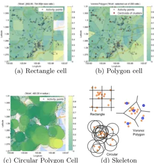
In Figure 2 (a), (b), and (c), the spatial activity frequency as calculated through equation (1) is depicted using real data for different cell types defined in the previous section. Colormap indicates a degree of the probability.
4.2.2
Distance based empirical probability
For each point pi, we obtain distance related features using
Euclidean distance. We define the distance between a point piand a set of points P as d(pi, pj) = min{kpi− pjk2: pj∈
P }. These features are calculated with respect to POIs, past activity information from all users and home and work from the specific user. Firstly, for cell ci containing the point pi
we obtain the contextual neighbor activity confidence P r(ai= l|Xl(ci)) := φ(d(pi, Xl(ci))) (2)
and the historical neighbor activity confidence
P r(ai= l|Al(ci)) := φ(d(pi, Al(ci))) (3)
where Xl(ci) is the activity set of type l from contextual
data (POIs) in cell ci, Al(ci) is the activity set of type
l from in cell ci, and φ(·) can be any activation function
such that it is normalized between 0 and 1. We have used φ(d) = (1 + d2)−1 which is the inverse of the squared dis-tance. (Also, a distance d is normalized between 0 and 1 for the points in the same cell).
Secondly, for each user u, we choose “core” activities (home and work), and calculate their core activity distance to pi.
(a) Rectangle cell (b) Polygon cell
(c) Circular Polygon Cell
Rectangle
Voronoi Polygon
Circular
(d) Skeleton
Figure 2: Empirical probability p(ai|ci) in (1) of Work
activity in spatial cells are shown: (a) rectangle cells, (b) polygon cells centroids of clusters, (c) circular cells at each activity point. (d) simplified explana-tion.
4.2.3
Activity Transition Probability
For each point pi, we obtain activity probability based
on the previous activity. The simplest way is to apply the first-order Markov chain where a current activity (a(t)) is conditioned on the value of most recent previous activity (a(t − 1)) in a transition distribution. We calculate the em-pirical transition probability:
P rsl(t − 1, t) = P r(a(t) = l|a(t − 1) = s) := PN j=1δaj (t),l·δaj (t−1),s PL l=1 PN j=1δaj (t),l·δaj (t−1),s, (4)
where N denotes the total number of activity points for all users u ∈ U , l denotes the current activity, s denotes the previous activity, l, s ∈ A (A is an activity set), and PL
l=1P rsl= 1.
We apply equation (4) to historical data to obtain transition probability matrix. Due to varying patterns during week-ends and weekdays, we obtain two transition matrices for corresponding periods. In practice, if there is no previous activity (no activity reported within 24 hours), we assume a uniform probability for each activity. We use these probabil-ity matrices to calculate the activprobabil-ity probabilprobabil-ity of current point pi.
4.2.4
Activity duration
For each point pi, we calculate its activity duration, Ti=
(ti2− ti1).
Acceleration and speed features are excluded since activity defined here is not about physical behavior such as walking, running, and so on [14]. These features are used to detect
stop segments in the FMS system as mentioned above. After the feature extraction process explained above we have the following feature vector, general features
x =[Temporal Activity Probability ∈ R1×L, Spatial Activity Probability ∈ R1×L, Contextual Activity Probability ∈ R1×L, Activity Transition Probability ∈ R1×L,
Historical Neighbor Activity Confidence ∈ R1×L, Contextual Neighbor Activity Confidence ∈ R1×L, Core Activity Distances ∈ R1×2,
Activity Duration ∈ R1]T∈ R6L+3
,
(5)
where L is the number of activity categories.
4.3
Classification
When the data is acquired from multiple sensors or sources (and then heterogeneous features are generated), a single classifier cannot find good decision boundary for classifica-tion [19]. To overcome this problem, in this section, we present ensemble learning based classification. Ensemble learning, here, is used through two levels; one is to learn heterogeneous features, and in second step, outputs from classifiers such as score and decision are merged to a final decision.
4.3.1
Ensemble decision trees
Ensemble learning has been widely used to cope with noisy real world data. In this paradigm, several (base) classifiers are learned from training data to eventually become a unified classifier. In theory, individual base classifiers can concen-trate on different areas of the problem space and, as a result, the unified classifier, which combines the output of those base models, becomes more robust. Two kinds of ensemble learning are used in this paper, namely bootstrap aggregat-ing (Baggaggregat-ing) and random subspace. In Baggaggregat-ing, each base classifier is trained with a subset generated by subsampling on the global training set. In the random subspace approach, each base classifier is learned using subspace features of the original feature set. To predict a class label for unseen data, a majority voting process is applied on the set of individual predictions.
Our base classifier will be decision trees, one of the pop-ular methods, which consist of gradually splitting the input feature space into decision regions. This method is useful to deal with irrelevant variables and is robust to outliers. How-ever, decision trees show unstable performance. To allevi-ate instability, ensemble learning has been widely adopted. One popular method is bagging of decision trees. Another powerful tool is a combination of aggregating set of random features (subspace) based on decision tree classifier, namely Random Forests [7].
Using a set of training features and activity labels {xi, ai} ∈
T r, ∀i where T r is a training set, we calculate an ensemble hypothesis function h(x, Θ) where Θ is a set of decision tree hypothesis θk, ∀k. This function finds an activity label a,
based on a = arg maxl sl, where sl is the score for
activ-ity label l. This function will be used to predict a label of unseen data xtest∈ T e for test in future.
4.3.2
Ensemble of user social demographic
charac-teristics based learning
Users with different social demographic characteristics show different activity and travel patterns [9, 13]. It is, thus, help-ful to learn a model using individual user’s history data, in addition to learning from other users’ history data. An in-dividual user belongs to multiple categories; formally each user is included in several different user sets: u ∈ U , P, O, G, where U denotes a cross (universal) user set, P denotes a specific user set, O denotes an age-specific user set, and G denotes a gender-specific user set. The input feature vec-tor of pi for a user u, x(pui), (where u ∈ U and xU, ∀u),
is generated based on subsets. Classifiers (hypotheses) are learned using user subsets: h(xU), h(xP), h(xO), and h(xG).
From each model, we get outputs such as 1) a score vector with a element sl ∈ [0, 1], ∀l for each class (activity) label
and 2) a decision dl, ∀l for the l-th class. The score of each
activity class from the hypothesis h(·) become an input fea-ture vector for ensemble classifier to determine a final score. Classifier’s decision can be merged by classifier learning and Weighted Majority Voting (WMV). WMV is one popular method to merge multiple decisions to obtain a final deci-sion (based on arg maxlPTt=1wtdt,l∀l where wt is a weight
for t-th classifier’s decision dt,l∈ {0, 1} for l-th class.) [19].
4.4
Workflows of the proposed algorithm
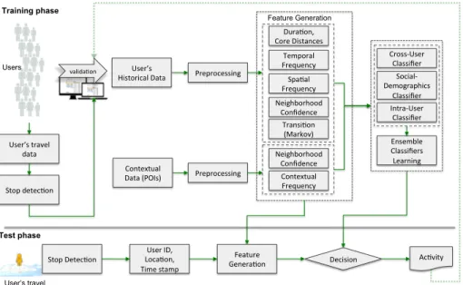
Figure 3 shows an overall flow of the proposed activity recognition system used in FMS. We infer an activity type for each user stop point.
5.
EXPERIMENTS
In this section, we evaluate the proposed algorithm using a dataset acquired through our FMS system.
5.1
Data set
Within the FMS, we have 793 users who have completed the survey with at least 5 validated days, as mentioned in Section 3.1. POI data has been provided by Singapore Land Authority (SLA). It has a total of 64, 819 points related to shopping malls, clinics, bus stops, and metro train stations, residential buildings, office buildings and so on2. These POIs
are mapped to our 16 activity categories. Table 1 shows the statistics for the mapping.
5.2
Data preprocessing and cleaning
As with any kind of survey, the data collected in FMS contains noise/errors, and this problem may be more seri-ous in this case than average. Since the FMS users were not guided by interviewer in their validation process, the task has been proven to be challenging to some of the users, es-pecially those less tech-savvy users. As a result, there can be multiple errors in user’s data. Therefore, data cleaning is an essential step before we perform any performance evalua-tion. Firstly, we select days where users started and finished their daily activity at home. Then, we apply a sequence of
2
POI label includes;e.g. Pub/Bar, Restaurant, Kiosk/Stall, Cafe,
Pet Shops, Child Care, Skin Care, Gym, Supermarkets, Convenience Stores, ATMs, MRT Stations, Swimming Complexes, Tuition Centres, Music Dance Schools, Car Wash, Toy Stores, Photography, Post Of-fices, Town Councils, HDB Branch OfOf-fices, Police Stations, Primary Schools, Secondary Schools, Hair Salons, Yoga Pilates, Accountants, Maid Agencies, Clinics, Laundry, Travel Agencies, Religious, Phar-macies, and so on.
Decision Dura,on, Core Distances Ac,vity Ensemble Classifiers Learning Spa,al Frequency Contextual Frequency Training phase Test phase valida,on Users Feature Generation Temporal Frequency Neighborhood Confidence Neighborhood Confidence Preprocessing User’s Historical Data Contextual Data (POIs) Feature Genera,on User ID, Loca,on, Time stamp Preprocessing Transi,on (Markov) Stop detec,on Stop Detec,on User’s travel data User’s travel Cross-‐User Classifier Social-‐ Demographics Classifier Intra-‐User Classifier
Figure 3: Overview of the proposed activity recognition system. Based on given an identified stop (detected by the current stop detection algorithm), the algorithm identifies an activity based on spatial, temporal, transition, and contextual features. We assume that his/her home location is known beforehand (provided when he/she registered in the website).
Table 1: The number of environmental context data per activity category generated based on Points of interest (POIs) which contain location information.
Activity #points percent (%)
Home 31 0.05
Work 48 0.08
Change Mode/Transfer 4965 8.25
Pick Up/Drop Off 0 0.00
Shopping 19862 32.99 Social 0 0.00 Work-Related Business 4619 7.67 Education 2678 4.45 Recreation 888 1.48 Medical/Dental (Self) 4150 6.89 Meal/Eating Break 10200 16.94 Entertainment 181 0.30 Sports/Exercise 529 0.88 Personal Errand/Task 12046 20.01 To Accompany Someone 0 0.00 Other’s Home 0 0.00 Other 4670 -*Other is excluded.
checks, and discard the data if home to home distance is higher than 50 meters; if home to other validated activities is less than 10 meters; or if activity points have swapped time between start and end of one activity. We also apply other filters: no activity with more than 24 hour duration is allowed; an activity outside of Singapore area is removed. As a result, we use 5,073 points from 243 users where their data had been collected from March 11th of 2013 to September 30th of 2013 for the following experiments.
5.3
Protocols and parameter settings
First, we apply two-fold validation where we keep the chronological order of data with k training days and one test day split, k = 1, 2, 3, 4 for every users. In the experiments, we apply different parameter settings: different resolutions
of time slot: [10, 20, 40, 60, 90, 120] minutes; different res-olutions of spatial cell width: [200, 400, 600, 800, 1000] me-ters; number of clusters for Voronoi polygons: [1000, 800, 600, 400, 200, 100]; Circle radii: [100, 150, 200, 300, 400, 500] meters.
For the random subspaces based decision trees (Random Forest (RF)), a dimension of subspace features is chosen based on square root of the total number of feature vari-ables. For decision tree-based (DT) classifiers including RF and bagging of DT (BagDT), the minimum number of obser-vations per tree leaf is set as 1. 100 base classifiers are used. A random seed found by pseudorandom number generation is fixed.
5.4
Results
5.4.1
Different resolutions of temporal slot and
spa-tial cell
Ensemble methods (BagDT and RF) show constant aver-age accuracy as temporal cell size increases. Accuracy value of those methods increases as spatial cell size increases for Rectangle and Voronoi Polygon cases. For more details, a reader can refer to [10].
5.4.2
Different number of training days
Figure 4 shows the average classification accuracy for dif-ferent number of training days. We see that the average accuracy is improved as the number of training days in-creases. In Figure 4 (a), individual classifier was learned using different sets of user population such as cross-user, individual user, age-specific user, and gender-specific user. The model using more training data shows better classifica-tion performance. Due to small number of training samples, user-specific model solely does not show best performance. However, that accuracy value drastically increases compared to other models as data size increases. In Figure 4 (b),
clas-sification performance of ensemble of individual models are shown. Ensemble models show better classification perfor-mance than that of individual models. Decision fusion based on weighted majority voting (weightedMvote) methods show stable and best performance along with the training days as shown in Figure 4 (b). 1 2 3 4 40 45 50 55 60 65 70 75 Average accuracy (%) training days Circular BagDT (cross−user) BagDT (user−spec) BagDT (age) BagDT (gender) RFs (cross−user) RFs (user−spec) RFs (age) RFs (gender)
(a) Individual Models
1 2 3 4 40 45 50 55 60 65 70 75 Average accuracy (%) training days Circular BagDT (scoreEnsemble) BagDT (decisionEnsemble) BagDT (weightedMVote) RFs (scoreEnsemble) RFs (decisionEnsemble) RFs (weightedMVote) (b) Fusion Models Figure 4: Average prediction accuracy along with number of training days for each model: (a) indi-vidual classifier learned using different sets of user population. (b) ensemble classifiers for merging in-dividual classifier models.
5.4.3
Relationship between activities and merging
In Table 2, we show classification confusion matrix for 16 activity categories. As shown in the table, most of the points in the Pick Up/Drop off class (PD) is classified as Change Mode/Transfer (C). Work-Related Business (WR) activities are mainly classified as Work (W). Many other activities (related to maintenance or discretionary context) are classified as Change Mode/Transfer (C) which has the largest training sample size. And this may relate to the fact that many shopping malls and shops are located close to street and bus/train stations in Singapore.
As the 16 activities cannot be exclusively explained, i.e. more than one activity can be tagged for one certain user stop point. We follow the work of [12, 20] to distill this set into a set of conceptually exclusive activities: 1) Home, 2) Work (including Work, Work-Related Business, and Educa-tion), 3) Transportation (including Change Mode/Transfer and Pick Up/Drop Off, and 4) Maintenance/Discretionary (including Meal/Eating Break, Shopping, Personal Errand/Task, Medical/Dental (Self ), and so on). Table 3 shows that clas-sification accuracy using four activity definition is improved compared to full sixteen activity categories.
5.4.4
Prediction performance improvement by
merg-ing of different sets of user population
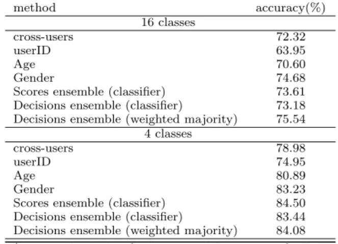
Table 3 shows classification accuracy for 16 classes and 4 classes respectively, using 4 training days and Random Forest with Rectangle cell type. Scores of multiple clas-sifier learned using different user population is merged by a classifier (Scores Ensemble by classifier). Decisions from multiple classifiers are merged by classifier (Decisions ensem-ble by classifier) and by Weighted Majority Voting. For the weighted majority voting (WMV), weights are simply deter-mined with ‘4’ for the cross-user model, ‘3’ for the gender model, ‘2’ for the age model, and ‘1’ for intra-user model. This is based on number of training samples per model;
General (total) > Gender > Age > User-specific. Decision merging with WMV shows consistently better classification accuracy than to other models.
Table 3: Overall accuracy (number correctly classi-fied/total number of samples), Random Forests
method accuracy(%) 16 classes cross-users 72.32 userID 63.95 Age 70.60 Gender 74.68
Scores ensemble (classifier) 73.61
Decisions ensemble (classifier) 73.18
Decisions ensemble (weighted majority) 75.54
4 classes
cross-users 78.98
userID 74.95
Age 80.89
Gender 83.23
Scores ensemble (classifier) 84.50
Decisions ensemble (classifier) 83.44
Decisions ensemble (weighted majority) 84.08
*setting: 4 training days, 800m × 800m rectangle size, 120 mins time slot.
*4 Classes: 1) Home, 2) Work, 3) Transportation, 4) Maintenance/Discretionary
5.4.5
Testing on real data stream and unseen user
effect
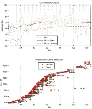
In Figure 5, we plot the test accuracy performance along with arrival of sequential data. The incoming unseen activ-ity data is predicted based on learned model using previous training data to obtain the test accuracy. Subsequently, this tested data is used for training in next sequence day based on its true (labelled by users) activity label. A test data is coming either from unseen user or seen user. Seen user means that his/her activity history is used during training models, and unseen user is not. As shown in the bottom figure in Figure 5, unseen users are appearing almost ev-ery days from multiple users. The top figure in Figure 5 shows accumulative accuracy of RF WMV where the val-ues are averaged for seen users (solid line) and unseen users (dashed line) respectively. By accumulative accuracy, we mean the average accuracy of the system from test day 1 to the current test day. We see that the classification accu-racy for seen users are better than unseen users which shows that learning from users’ own history helps to improve the classification accuracy. Classification performance of unseen users improves as the training day accumulates more than that of seen users. For test classification of unseen user, the model learned from cross-user and users from social-demographics are used. Since there are more number of training data from cross-user and social demographics based users than user-specific information, the performance could be improved relatively larger than that of seen user case.
To observe the effect of number of user-specific training days further, average classification accuracy is shown along with user-specific training days again. Different from set-tings in Figure 4, every user has different total number of training days for learning in Figure 6. Training days ‘0’ in-dicates that no user-specific data is used in training for that user (unseen user). In Figure 6, an average accuracy value increases as number of user-specific training days increases.
Table 2: Confusion matrix: Random Forests (RF) prediction of Table 3
truth \predict H W C PD Sh So WR E R MD M E Sp P A OH accuracy (%)
H 63 0 0 0 0 0 0 0 0 0 0 0 0 0 0 0 100 W 3 105 10 0 0 0 0 0 0 0 1 0 0 0 0 0 88.24 C 0 1 147 0 0 0 1 0 0 0 1 0 0 2 0 0 96.71 PD 0 0 3 1 0 0 0 0 0 0 1 0 0 1 0 0 16.67 Sh 0 1 7 0 1 0 1 0 0 0 3 0 0 0 0 0 7.69 So 0 2 7 0 0 0 0 0 0 0 2 0 0 0 1 0 0 WR 0 8 5 0 0 0 0 0 0 0 1 0 0 0 0 0 0 E 1 4 3 0 0 0 0 1 0 0 1 0 0 0 0 0 10.00 R 0 0 1 0 0 0 0 0 0 0 0 0 0 0 0 0 0 MD 0 0 0 0 0 1 0 0 0 0 1 0 0 0 0 0 0 M 0 5 13 0 1 0 2 0 0 0 29 0 0 1 0 0 56.86 E 0 0 0 0 0 0 0 0 0 0 1 0 0 0 0 0 0 Sp 0 0 0 0 0 1 1 0 0 0 0 0 0 0 0 0 0 P 0 2 7 0 0 0 2 0 0 0 0 0 0 4 2 0 23.53 A 0 1 1 0 0 0 0 0 0 0 0 0 0 0 1 0 33.33 OH 0 0 0 0 0 0 0 0 0 0 0 0 0 0 0 0 -Overall 75.54
Home (H), Work (W), Change Mode/Transfer (C), Pick Up/Drop Off (PD), Shopping (Sh), Social (So), Work-Related Business (WR), Education (E), Recreation (R), Medical/Dental (MD), Meal/Eating Break (M), Entertainment (E), Sports/Exercise (Sp), Personal Errand/Task (P), To Accompany Someone (A), Other’s Home (OH)
20 40 60 80 100 120 30 40 50 60 70 80 90 100 accuracy (%) Classification; Circular day RFs RFs − Seen RFs − Unseen 20 40 60 80 100 120 400 600 800 1000 1200 1400 1600 user ID day Unseen/Seen users distribution
Unseen Seen
Figure 5: Test accuracy performance along with ar-rival of sequential data. The incoming unseen activ-ity data is predicted based on learned model using previous training data to obtain the test accuracy. First day test is conducted when a model is learned with 3 training days data.
To avoid a biased result, test results involving more than 30 users at that day are shown. Decay value at day 1 is related to bias effect from small individual user sample size. A rea-son of decay at training day 5 in Figure 6 (a) may be found from that the number of test cases are relatively more than the number of the users. Ratio (number of test samples ver-sus number of test users) at training days 5 (including day 1) is relatively higher than other cases3. It means that each user has more activity points than other cases in average, so
3
Ratio at day 5 is 5.92 and 5.8 at day 1. Average of others [0,2,3,4,6,7] days is 4.84. Ratio = [4.1667, 5.8010, 4.9597, 5.0088, 5.1084, 5.9206, 5.1818, 4.6176].
more unseen/unusual activity patterns would be included in that day 5 case than other cases.
Most of users have less than 3 training days as shown in Figure 6 (b). If more individual users have more training days, overall accuracy of seen user (in Figure 5) could be improved. We can observe that average accuracy keep im-proves as training days increases in Figure 6 (a).
0 1 2 3 4 5 6 7 50 60 70 80 90 100
Number of training days
Average accuracy (%) BagDT RFs (a) Prediction 0 1 2 3 4 5 6 7 0 5 10 15 20 25 30 Percentage (%)
Number of training days Number of users Number of cases
(b) Number of users and cases Figure 6: (a) Averaged accuracy along with the number of user-specific training days for individual users. (b) Corresponding number of users and test cases during testing
6.
CONCLUSIONS
In this paper, we proposed a framework to recognize an activity type of a traveler when his/her movement is tracked by mobile sensors, as per our Future Mobility Survey (FMS) technology [3]. With different shapes of spatial quantization, ensemble classifiers are applied to process noisy real-world spatial-temporal and contextual data. To improve general-ization performance, our model takes advantage of cross-user historical data as well as user-specific information, includ-ing social demographic characteristics. Fusion of multiple classifiers learned from different user populations shows im-proved generalization performance than that of individual classifier learning. We evaluated the activity classification performance along with sequential data for a real life situ-ation. As the number of training data is accumulating, the generalization performance is improved. Also, we demon-strated that learning from a user’s own history improves the recognition accuracy. Our empirical results demonstrate that the proposed method contributes significantly to our travel survey application.
In terms of future work, there are several potential avenues for investigation. To find the centroids of Voronoi polygon,
more adaptive spatial clustering techniques such as hierar-chical clustering and density based clustering could be used [16, 11]. We can compare between pointwise classification (deployed in the current system) and sequence based classi-fication (HMM, CRF, etc.) which is workable for continuous travel data environment. Finally, we can assess the positive feedback cycle between the algorithm and user labeling to improve classification performance in future survey.
7.
ACKNOWLEDGMENTS
This research was funded by the Singapore National Re-search Foundation (NRF) through the Singapore-MIT Al-liance for Research and Technology (SMART) Center for Future Urban Mobility (FM) Group. The authors would like to thank FMS team (Bruno, Inˆes, Kalan, Rui) for their support and give special thanks to Rudi Ball and Carlos Carrion for their data cleaning effort.
8.
REFERENCES
[1] K. W. Axhausen, S. Schonfelder, J. Wolf, M. Oliveria, and U. Samaga. Eighty weeks of gps traces,
approaches to enriching trip information. In 83rd Annual Meeting of the Transportation Research Board, 2004.
[2] W. Bohte and K. Maat. Deriving and validating trip purposes and travel modes for multi-day gps-based travel surveys: A large-scale application in the netherlands. Transportation Research Part C, 9:285–297, 2009.
[3] C. Cottrill, F. Pereira, F. Zhao, I. Dias, H. Lim, M. Ben-Akiva, and P. Zegras. Future mobility survey: Experience in developing a smartphone-based travel survey in singapore. Transportation Research Record: Journal of the Transportation Research Board, 2354(-1):59–67, 12 2013.
[4] Z. Deng and M. Ji. Deriving rules for trip purpose identification from gps travel survey data and land use data: A machine learning approach. In Seventh International Conference on Traffic and Transportation Studies (ICTTS), 2010.
[5] D. Feldman, A. Sugaya, C. Sung, and D. Rus. idiary: From gps signals to a text-searchable diary. In Proceedings of the 11th ACM Conference on Embedded Networked Sensor Systems, SenSys ’13, pages
6:1–6:12, New York, NY, USA, 2013. ACM. [6] B. Furletti, P. Cintia, C. Renso, and L. Spinsanti.
Inferring human activities from gps tracks. In Proceedings of the 2nd ACM SIGKDD International Workshop on Urban Computing, UrbComp ’13, pages 5:1–5:8, New York, NY, USA, 2013. ACM.
[7] T. K. Ho. The random subspace method for constructing decision forests. IEEE Transactions on Pattern Analysis and Machine Intelligence,
20(8):832–844, 1998.
[8] L. Huang, Q. Li, and Y. Yue. Activity identification from gps trajectories using spatial temporal pois’ attractiveness. In Proceedings of the 2Nd ACM SIGSPATIAL International Workshop on Location Based Social Networks, LBSN ’10, pages 27–30, New York, NY, USA, 2010. ACM.
[9] S. Jiang, J. Ferreira, and M. C. Gonz´alez. Clustering daily patterns of human activities in the city. Data
Mining and Knowledge Discovery, 25(3):478–510, 2012.
[10] Y. Kim, F. C. Pereira, F. Zhao, A. Ghorpade, P. C. Zegras, and M. Ben-Akiva. Activity recognition for a smartphone based travel survey based on cross-user history data. In Proceedings of the 22nd International Conference on Pattern Recognition (ICPR‘14), 2014. [11] S. Kisilevich, F. Mansmann, M. Nanni, and
S. Rinzivillo. Spatio-temporal clustering. In
O. Maimon and L. Rokach, editors, Data Mining and Knowledge Discovery Handbook, pages 855–874. Springer US, 2010.
[12] A. Kulkarni and M. G. McNally. A microsimulation of daily activity patterns. Technical report, Institute of Transportation Studies, University of Califonia, Irvine., 2000.
[13] M.-P. Kwan. Gender and individual access to urban opportunities: A study using space–time measures. The Professional Geographer, 51(2):211–227, 1999. [14] J. R. Kwapisz, G. M. Weiss, and S. A. Moore.
Activity recognition using cell phone accelerometers. SIGKDD Explor. Newsl., 12(2):74–82, Mar. 2011. [15] L. Liao, D. Fox, and H. Kautz. Location-based
activity recognition using relational markov networks. In Proceedings of the 19th International Joint
Conference on Artificial Intelligence, IJCAI’05, pages 773–778, San Francisco, CA, USA, 2005. Morgan Kaufmann Publishers Inc.
[16] S. Liu, Y. Liu, L. M. Ni, J. Fan, and M. Li. Towards mobility-based clustering. In Proceedings of the 16th ACM SIGKDD International Conference on Knowledge Discovery and Data Mining, KDD ’10, pages 919–928, New York, NY, USA, 2010. ACM. [17] M. May, B. Berendt, A. Cornu´ejols, J. Gama,
F. Giannotti, A. Hotho, D. Malerba, E. Menesalvas, K. Morik, R. Pedersen, L. Saitta, Y. Saygin, A. Schuster, and K. Vanhoof. Research challenges in ubiquitous knowledge discovery. In Next Generation of Data Mining. CRC, 1 edition, 2008.
[18] F. C. Pereira, C. Carrion, F. Zhao, C. Cottrill, C. Zegras, and M. Ben-Akiva. The future mobility survey: Overview and preliminary evaluation. In Proceedings of the Eastern Asia Society for Transportation Studies, 2013.
[19] R. Polikar. Ensemble Based Systems in Decision Making. IEEE Circuits and Systems Magazine, 6(3):21–45, 2006.
[20] W. W. Recker, M. G. McNally, and G. S. Root. Travel/activity analysis: Pattern recognition, classification and interpretation. Transportation Research Part A: General, 19(4):279 – 296, 1985. [21] C. Song, T. Koren, P. Wang, and A.-L. Barabasi.
Modelling the scaling properties of human mobility. Nature Physics, 6(10):818–823, Sept. 2010.
[22] P. R. Stopher, C. FitzGerald, and J. Zhang. Search for a global positioning system device to measure person travel. Transportation Research Part C, 15:350–369, 2008.
[23] J. Wolf, R. Guensler, and W. Bachman. Elimination of the travel diary: an experiment to derive trip purpose from gps travel data. In 80th Annual Meeting of the Transportation Research Board, 2001.
View publication stats View publication stats