Deposition and Dispersion of Inertial Aerosols in
Secondary and Turbulent Flow Structures
by
Kurt W. Roth
Submitted to the Department of Mechanical Engineering
in partial fulfillment of the requirements for the degree of
Doctor of Philosophy
at the
MASSACHUSETTS INSTITUTE OF TECHNOLOGY
February, 1995
© Massachusetts Institute of Technology, 1995. All Rights Reserved.
Author ...
...
Mechanical Engineering
.ntmber
29th, 1994
/.D
...
o
f eanica.. l Engineri
Dept. of Mechanical Engineering
John H. Lienhard V
Accepted by ...
Ain A. Sonin
Professor of Mechanical Engineering
Department of Mechanical Engineering
ed by
Deposition and Dispersion of Inertial Aerosols in Secondary and
Turbu-lent Flows
by Kurt W. Roth
Submitted to the Department of Mechanical Engineering on
Sep-tember 29th, 1994, in partial fulfillment of the requirements for the
degree of Doctor of Philosophy in Mechanical Engineering
Abstract
Aerosol deposition in secondary flows poses a challenging problem in several engineering applications. For example, particles in the wake of heat exchanger tube bundles or weld seams in fluidized bed combustors can severely erode the wall surfaces. This studs'
exam-ines the deposition of inertial aerosols (Sauter mean diameter greater than 40lm) behind a
blunt plate mounted on a long splitter plate, i.e. a T-step configuration. Deposition rates
are measured using a novel Laser-Induced Fluorescence (LIF) technique both in the
recir-culation region immediately behind the T-step (secondary flow) and the approximately plane mixing layer following flow reattachment. The parameters of step height, mean flow velocity, and particle diameter are varied to obtain deposition rates for over two orders of magnitude in Stokes Number.
Aerosol deposition in the recirculation zone is strongly depressed relative to the post-recirculation mixing layer region and a flat plate turbulent boundary layer. Particle number density profile measurements indicate that the low secondary flow deposition rates occur
because the particles possess too much inertia to successfully negotiate the streamline
cur-vature at the T-step and become entrained in the secondary flow. In addition, aerosol depo-sition rates do not appear to scale well with the secondary flow eddy-turnover timescale, i.e. with xr/U.
Deposition in the post-reattachment approximate plane mixing layer scales quite well with the local fluctuating velocity normal to the wall, i.e v'. The plane mixing layer deposition rates also appear to lie below those found in a turbulent boundary layer; however, when the local number density is taken into account, the deposition rates then agree with the
tur-bulent boundary layer deposition rates. This implies that secondary flow deposition rates
cannot be estimated by knowledge of but global flow qualities; the flow and its effect upon
the dispersion and resulting aerosol distribution must also be understood. Gravity appears
to have a negligible effect upon the deposition rate in all the cases examined.
LIF deposition measurements in a turbulent boundary layer agree well with past measure-:ments and establish the validity of the LIF technique.
Velocity response experiments performed in the decaying turbulence field behind a
biplane grid displayed qualitative evidence of the "convective crossing trajectories effect".
flow convecting the inertial particles from a region of higher turbulent intensity to lower
intensity while the decay of the particle turbulent intensity lagged that of the flow field.
Additional efforts revealed that the Aerometrics' Phase Doppler Particle Analyzer (PDPA)
has a "background" rms velocity of about 1.5%, and that this error is highly dependent
upon particle diameter and photomultiplier voltage.
Thesis Supervisor: John H. Lienhard V
Acknowledgments
It is an oft-used cliche that there were numerous people behind the efforts represented in this thesis. In this instance, it would be difficult to understate the contributions and support that many others have given me. I would like to thank:
My advisor, John H. Lienhard V, known better to me as "John." He has been an excellent advisor, who always has been generous with his time, knowledge and insight. and his guidance throughout the evolution of this thesis has been most valuable. I also feel very fortunate to have had an advisor who is a human being, who believes in an equal and open
relationship with his students, and respects his students and their interests. Thank you,
John!
The members of the Heat Transfer Lab over my three years here for their kindness and
helpfulness, in particular, my office mates: Jorge "Luis" Colmenares, Malcolm Child,
Laurette Gabour, Mike Feng, Jim "Clutch" Nowicki and Andy Pfahnl. They deserve
spe-cial appreciation for putting up with me when I would regress into a self-absorbed funk. I
also appreciate In addition, the Block & Tackle team members, including Pat Griffin,
Keith "HA, HA!" Crowe, Mike Lints, Peter Hinze and Detlef Westphalen, gave me a
weekly lift every summer.
Ed Lanzilotta and Tim Quinn. Together, we overcame qualifying exams and also forged a
strong friendship. May we continue to hold "quals meetings"!
Prof. Peter Griffith and Prof. Roger Kamm, for offering their advice and serving on my
thesis committee. Dr. James D. Blanchard of the Harvard School of Public Health, in
addi-tion to participating in my thesis committee, was always more than willing to share his
advice with me and has given me much practical insight into aerosol science.
Further-more, he kindly allowed me to borrow the MAGE and VOAG aerosol generators for
extended periods of time.
Norman Berube for sharing his gifts of design and machining insight with me on
numer-ous occasions. I owe the construction of the spinning disks and the test section portals to his manufacturing ideas, his ability to teach and his patience.
Norm McAskill and Dick Fenner for their help and good cheer.
There is so much more to life than engineering, and the music program at MIT has greatly
enriched my life and provided sustenance when my research was not progressing as well
as I would have liked. I have grown to love chamber music, and have particularly enjoyed making music with Leonard Kim and Richard Olson, and above all Mary Beth Rhodes,
whose playing inspires me and brings the sun through the clouds. I have also grown much
as not only a 'ellist but also as a musician through 'cello lessons from Michael Curry and the coachings of Prof. John Harbison. I would also like to thank the MIT music
The completion of this dissertation completes a process that began over twenty years ago. One often hears of the critical part that role models and mentors play in achievement in science, and I have been most fortunate in this regard. From the beginning, my father and my mother have always encouraged and challenged me to learn and achieve, be it reading to me, helping me with homework, or giving me their support and unqualified love. I became interested in engineering at Mount Hebron High School, where Dave Oppelt taught me physics my junior and senior years. "Doc Op's" unique teaching style, a fusion of enthusiasm and didactic labs, aroused my interest in mechanics and convinced me to attend M.I.T. At M.I.T., I decided to pursue fluid mechanics after taking 2.20 taught by Prof. Probstein. During my junior year, I participated in my first UROP with Prof. Patera.
The following summer, I became immersed in fluid mechanics research working with Prof. Leehey in the Acoustics & Vibration Lab wind tunnel. His patience, willingness to challenge me and his collegial modus operantis made research a joy and Prof. Leehey the ideal mentor. It is primarily due to his generosity that I decided to pursue graduate work in fluid mechanics. Graduate student Kay Herbert helped to make this a special experience.
Buoyed by an exciting Masters' thesis project, also under the supervision of Prof. Lee-hey, I decided to remain in graduate school and pursue a doctorate.
The one overreaching constant throughout this experience and, indeed, my life, has been my family. My Mom, my Dad, and my brother Peter have been so loving understand-ing, in both good times and bad, and I know that I will always have a place, a family, that I can call home. I love them without reserve, and it is to my family that I dedicate this the-sis.
I would like to thank the NSF, under Grant CBTE 88-58288, the Electric Power Research Institute, Grant RP8000-41, and the NIEHS for their financial support.
Table of Contents
A bstra ct ... ... 2
A cknow ledgm ents ... 4
Table of C ontents ...6
L ist of Figures ... ... 9
List of Tables ... 14
Nomenclature
...
15
1 Introduction ... 18
1.1 The Contexts of Aerosol Deposition ... 19
1.2 Overview of Aerosol Dispersion ... 1
1.3 The Essential Problem ...
21
2 Instrumentation ...
24
2.1 Aerosol Wind Tunnel Facility ... 24
2.2 Hot-Wire Anemometry ...
27
2.2.1 A/D Discretization Error ...
28
2.3 Phase Doppler Particle Anemometry ... 29
2.4 Deposition Measurement ...
33
2.5 The LIF Deposition Measurement Technique ...34
2.6 Calibration of the LIF System ... 36
2.6. 1 Photo-Bleaching of Deposited Fluorescein ...37
2.7 Surface Flow Visualization ... 37
3 Aerosol Generation ... 45
3.1 Test Aerosol Parameters ... 45
3.2 Particle Sizing Parameters and Measures of Monodispersity ... 46
3.3 Liquid Spray Atomizers ... 48
3.3.1 Pressurized Air and Water Liquid Atomizer ...48
3.3.2 Compressed Air Nebulizer ...
49
3.4 Vibrating Orifice Aerosol Generator (VOAG) ... 51
3.5 Condensation Monodisperse Aerosol Generator ...53
3.6 Spinning Disk Aerosol Generator ...
55
3.6.1 Performance Characteristics of the Spinning Disk Generator ...57
3.7 Two-Dimensional High-Power Acoustic Droplet Generator:
The Array Generator ... 613.7.1 Unclogging the Array Generator Orifices ... 62
3.7.2' Dispersion Air .
...
63
3.7.3 Array Generator Performance ...
64
3.7.4 Array Generator Aerosol Solution ... 65
3.8 Summary of Aerosol Generation Techniques ... 67
3.9 Aerosol Evaporation ... 67
3.10 Evaporation Experiments ... 69
4 Particle Velocity-Response Experiments ...
...82
4.1 Overview ... 82
4.2 The Scaling of Particle Velocity-Response ... 82
4.2.1 Equation of Motion for a Single Particle ... 83
4.2.2 Particle Time Scale ...
84
4.3 Flow Time Scale ... 86
4.4 Models for Particle Velocity Response ... 87
4.4.1 Ve locity Response Augmentation ... 88
4.4.2 Comparison of Experiment with Numerical Models ...90
4.5 Bi-plane Grid Turbulence Experiments ... 91
4.5.1 The "Convective Crossing Trajectories Effect"...94
4.6 Detailed Grid Turbulence Experiments ... 95
4.7 Investigation of Particle Response Notches ... ...98
4.7.1 PDPA Operation on Track 2 ... 98
4.7.2 Aerometrics' Assessment of Track 2 versus Track 3
... 100
4.7.3 Open Tunnel Runs ... ... 100
4.7.4 Track 3 Open Channel Runs ... 102
4.7.5 Viability of Track 3 Results ... 102
4.8 Conclusions ... 103
5 Deposition in Secondary Flow ... 137
5.1 Overview ... 137
5.2 Turbulent Inertial Deposition and Deposition Velocity ... 138
5.2.1 Past Turbulent Deposition Results ...140
5.3 Step Flows
...
141
5.4 Secondary Flow Behind a T-Step ... 142
5.4.1 Mean Flow ... 142
5.4.2 Two-Dimensionality of Flow ...
143
5.4.3 Turbulence Quantities ...
144
5.5 Present T-Step Configuration ...
145
5.5.1 Reattachment Length ... 146
5.6 Particle Deposition Experiment Protocol ... 147
5.6.1 Particle Evaporation Correction
.
.
...
149
5.7 Turbulent Boundary Layer Deposition Rates
...
... 150
5.8 The T-Step Flow: PDPA Particle Statistics Measurements ... 152
5.8.1 Mean Velocity Profiles ... 153
5.8.2 Fluctuating Velocity Profiles ... 154
5.8.3 Particle Number Density Profiles ... 155
5.8.4 Sauter Mean Diameter Profiles ... 158
5.9 Secondary Flow Deposition Results ... 159
5.9.1 A Global View of Aerosol Deposition: By Step Height ... 160
5.9.2 A Global View of Aerosol Deposition: By Reference Velocity ... 161
5.10 The Scaling of Deposition in the Recirculation Region ... 162
5.10.1 Eddy Turnover Timescale ...
162
5.10.2 Turbulent Timescale ... 163
5.11 Scaling of Deposition in the Region Downstream of Recirculation ... 165
5. 12 Conclusions ... 168
B ibliography ... 243
B.1 Safety Concerns and Stress Calculations ... 253
B.2 Spinning Disk Construction ...254
Appendix C: The Pythagorean Velocity Error Correction Technique ... 255
Appendix D: PDPA Error Assessment ...257
D.1 Baseline RMS-Velocity Error ...
257
D. 1.1 Water Droplet Experiments ...
... 257
D. 1.2 Oil Droplet Experiments ... 258
D.2 PDPA Hardware Errors ...
259
D.2.1 Laser Beam Quality on Tracks One and Three ... 259
D.2.2 Ramifications for Earlier Track Three Experiments
... 260
D.3 Published PDPA Error ...261
D.3.1 Published Error Analysis of PDPA: Particle Sizing
...261
D.3.2 Published Error Analysis of PDPA: Number Density
...263
D.4 Other PDPA Errors ...
263
D.4.1 Velocity Discretization Error ...263
D.4.2 PDPA Error and Wall Contamination ...
...
264
D.4.3 Low-Frequency Mean Velocity Variation ... 264
Appendix E: Channel Flow Experiments ... 271
E. 1 The Channel Flow ... 271
E.2 Channel Flow Geometry ... 273
E.3 Challenges of Channel Flow Velocity Response Experiments ... 273
E.4 Dependence of Velocity Response Upon PMT Voltage ... 275
Appendix F: Ultrafine Aerosol Deposition ... 280
F. 1 Overview ... 280
F.2 The Ultrafine Aerosol Wind-Tunnel ...
280
F.3 Ae:rosol Seeding ... 281
F.4 Secondary Flow Model ... 283
F.5 TEM Technique ...
284
F.6 Experimental Protocol ...
...
286
F.7 Results ... 287
F.8 Unknowns and Sources of Error ...
288
2.1: The Heat Transfer Lab Aerosol Suction Wind-Tunnel ... 39
2.2: The LIF Deposition Measurement System ... 40
2.3: The LIF Fiber-Optic Cable System ... 41
2.4: The LIF Calibration System ... 42
2.5: A LIF Calibration Curve,
I0cft
vs. VPMT ... 432.6: Photobleaching Effect Upon Deposited Uranine Layer; Io= 1.4mW ... 44
3.1: Particle Size Distribution of Vortec SprayVector in
Grid Turbulence Experiments ...
...
72
3.2: Schematic of Vibrating Orifice Aerosol Generator (VOAG) ... 73
3.3: Schematic of Monodisperse Aerosol Generator (MAGE) ...74
3.4: MAGE Particle Diameter as a Function of Flow Rate
and Temperature ... 753.5: The Spinning Disk System ...
76
3.6: The Array Generator System ...
77
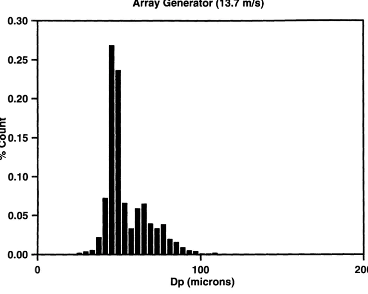
3.7a: Particle Size Distribution of the Array Generator (AG); mode 1 ... 78
3.7b: Particle Size Distribution of the Array Generator (AG); mode 2 ... 79
3.8: Aerosol Generator Characteristics ... 80
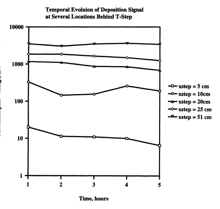
3.9: Temporal Evolution of Deposition Signal at Several Locations Behind the T-Step ... 81
4.1: The Spatial Decay of Grid-Turbulence; A=46.2, n= 1.086 ... 104
4.2: Initial Grid Turbulence Particle Response Experiments at
Several x/M Locations; uncorrected for PDPA error ... 1054.3: Initial Grid Turbulence Fluctuating Particle Velocities versus dp from x/M= 16 to 30; uncorrected for PDPA error ... 106
4.4: Particle Velocity-Response for x/M=16-30; corrected for PDPA error ... 107
4.5: Graphical Representation of the "Convective Crossing
Trajectories Effect" ...
108
4.6a:
4.6b:4.6c:
4.6d:
4.6e:4.6f:
4.6g:4.6h:
4.6i:
4.7a: 4.7b: 4.7c: 4.7d: 4.7e: 4.7f: 4.7g: Grid Turbulence Particle Velocity Response versus Stk, x/M=16 ... 109Grid Turbulence Particle Velocity Response versus Stk, x/M= 18 ... 110
Grid Turbulence Particle Velocity Response versus Stk, x/M=20 ... 11ll
Grid Turbulence Particle Velocity Response versus Stk, x/M=22 ... 112
Grid Turbulence Particle Velocity Response versus Stk, x/M=24 ... 113
Grid Turbulence Particle Velocity Response versus Stk, x/M=26 ... 114
Grid Turbulence Particle Velocity Response versus Stk, x/M=28 ... 115
Grid Turbulence Particle Velocity Response versus Stk, x/M=30 ... 116
Grid Turbulence Particle Velocity Response versus Stk, x/M=32 ... 117
Grid Turbulence Particle Velocity Response versus dp, x/M=16 ... 118
Grid Turbulence Particle Velocity Response versus dp, x/M=18 ... 119
Grid Turbulence Particle Velocity Response versus dp, x/M=20 ... 120
Grid Turbulence Particle Velocity Response versus dp, x/M=22 ... 121
Grid Turbulence Particle Velocity Response versus dp, x/M=24 ... 122
Grid Turbulence Particle Velocity Response versus dp, x/M=26 ...123
Grid Turbulence Particle Velocity Response versus dp, x/M=28 ... 124
List of Figures
FigureFigure
Figure
Figure
Figure
FigureFigure
Figure
Figure
Figure
Figure
Figure FigureFigure
Figure FigureFigure
FigureFigure
FigureFigure
FigureFigure
Figure
FigureFigure
Figure
Figure
Figure
Figure
Figure
Figure
Figure
Figure
Figure
Figure
Figure
Figure 4.7h: Grid Turbulence Particle Velocity Response versus dp, x/M=30 ... 125
Figure 4.7i: Grid Turbulence Particle Velocity Response versus dp, x/M=32 ... 126
Figure 4.8a: Track 2 Grid Turbulence Particle Velocity Response
versus dp, x/M=20 ...
127
Figure 4.8b: Track 2 Grid Turbulence Particle Velocity Response
versus dp, x/M=22 ...
128
Figure 4.8c: Track 2 Grid Turbulence Particle Velocity Response
versus dp, x/M=30 ...
129
Figure 4.9a: Comparison of Track 2 and Track 3 Grid Turbulence Intensities
versus dp, x/M=22; uncorrected for PDPA error ...130
Figure 4.9b: Comparison of Track 2 and Track 3 Grid Turbulence Intensities
versus dp, x/m=22; corrected for PDPA error ...
... 131
Figure 4.9c: Comparison of Track 2 and Track 3 Particle Velocity-Response
versus dp, x/M=22; corrected for PDPA error ...132
Figure 4.10a: Track 3 Grid Turbulence Particle Velocity-Response
versus dp, with n=l, x/M=20 ...
133
Figure 4.1 Ob: Track 3 Grid Turbulence Particle Velocity-Response versus dp, with n=1, x/M=22 ... 134
Figure 4. 10c: Track 3 Grid Turbulence Particle Velocity-Response
versus dp, with n=1, x/M=24 ...
135
Figure 4.10d: Track 3 Grid Turbulence Particle Velocity-Response versus dp, with n= 1, x/M=30 ... 136
Figure 5.1: Deposition Rates for Droplets in a Turbulent Flow ... 171
Figure 5.2: Eddy Deposition Rates of Particles on Smooth Surfaces ... 172
Figure 5.3: Diagram of the T-Step Tunnel Geometry ... 173
Figure 5.4: Three-Dimensional View of T-Step Secondary Flow ... 174
Figure 5.5a: Surface Flow Visualization Behind the T-Step,
hs=1.27cm, U=12.65m /s ...177
Figure 5.5b: Surface Flow Visualization Behind the T-Step,
hs=2.54cm, U=9.70m/s .
...
... 178
Figure 5.5c: Surface Flow Visualization Behind the T-Step (Reattachment Zone)
hs=1.27cm, U=12.65m.s ...
179
Figure 5.5d: Surface Flow Visualization Behind the T-Step,
hs=2.54cm, U=3.5m.s ...
180
Figure 5.6a: Deposition Rate Data Uncorrected for Change in
Fluorescein Concentration ...
181
Figure 5.6b: Deposition Rate Data Corrected for Change in
Fluorescein Concentration ...
182
Figure 5.7: LIF Particle Deposition Rates in a Turbulent Boundary Layer,
KD/U versus
...
183
Figure 5.8a: T-Step Mean Velocity Profiles, U/Ur versus y,
hs=2.54cm, Ur=4.15m s ... 184Figure 5.8b: T-Step Mean Velocity Profiles, U/Ur versus y,
hs=2.54cm, Ur=7.54m/s ...
185
Figure 5.8c: T-Step Mean Velocity Profiles, U/Urversus y, 186 hs=0.64cm, Ur= 11.55m/s ... 186
Figure 5.9a: T-Step Mean Velocity Profiles: U/Ur versus y,
hs=1.27cm, Ur=3.88m /s ... 187 Figure 5.9b: T-Step Mean Velocity Profiles: U/Ur versus y,
hs=1.27cm, Ur=8. 15m /s ... 188 Figure 5.9c: T-Step Mean Velocity Profiles: U/Ur versus y,
hs= 1.27cm, Ur= 12.27m/s ... 189 Figure 5.10a: T-Step Mean Velocity Profiles: U/Ur versus y,
hs=0.64, U r=3.92m/s ... 190 Figure 5.10b: T-Step Mean Velocity Profiles: U/Ur versus y,
hs=0.64cm, Ur=8.32m /s ... 191 Figure 5. 10c: T-Step Mean Velocity Profiles: U/Ur versus y,
hs=0.64cm, Ur= 12.63m/s ... 192
Figure 5.1 la: T-Step Fluctuating Velocity Profiles, u'/Ur versus y,
hs=2.54cm , Ur=4. 15m /s ... 193
Figure 5.1 lb:: T-Step Fluctuating Velocity Profiles, u'/Ur versus y,
hs=2.54cm , Ur=7.54m /s ... 194 Figure 5.1 lc: T-Step Fluctuating Velocity Profiles, u'/Ur versus y,
hs=2.54cm, Ur= 11.55m/s ... 195
Figure 5.12a: T-Step Fluctuating Velocity Profiles, u'/Ur versus y,
hs= 1.27cm , U r=3.88m/ s ... 196 Figure 5.12b: T-Step Fluctuating Velocity Profiles, u'/Ur versus y,
hs=1.27cm, Ur=8.15m/s .
...
... 197
Figure 5.12c: T-Step Fluctuating Velocity Profiles, u'/Ur versus y,
hs=1.27cm , Ur= 12.27m /s ... 198 Figure 5.13a: T-Step Fluctuating Velocity Profiles, u'/Ur versus y,
hs=0.64cm, Ur=3.92 ...
199
Figure 5.13b: T-Step Fluctuating Velocity Profiles, u'/Ur versus y,
hs=0.64cm, Ur=8.32m/s ... 200
Figure 5.13c: T-Step Fluctuating Velocity Profiles, u'/Ur versus y,
Ihs=0.64cm, Ur= 12.63m/s ... 201 Figure 5.14a: T-Step Number Density Profiles, ND/NDr versus y,
hs=2.54cm, Ur=4.15m/s ... 202 Figure 5.14b: T-Step Number Density Profiles, ND/NDr versus y,
hs=2.54cm, Ur=7.54m/s ... 203 Figure 5.14c: T-Step Number Density Profiles, ND/NDr versus y,
hs=2.54cm, Ur= 1.55m/s ...
204
Figure 5.15a: T-Step Number Density Profiles, ND/NDr versus y,
hs=1.27cm, Ur=3.88m/s ... 205
Figure 5.15b: T-Step Number Density Profiles, ND/NDr versus y,
hs=1.27cm, Ur=8.15m/s ... 206 Figure 5.15c: T-Step Number Density Profiles, ND/NDr versus y,
h
s=1.27cm, Ur=12.27m/s .
...
207
Figure 5.16a: T-Step Number Density Profiles, ND/NDr versus y,
hs=0.64cm, Ur=3.92m/s ... 208 Figure 5.16b: T-Step Number Density Profiles, ND/NDr versus y,
Figure 5.16c: T-Step Number Density Profiles, ND/NDr versus y,
.hs=0.64cm, Ur=12.63m/s ... 210
Figure 5.17a: T-Step Sauter Mean Diameter Profiles, d32 versus y, hs=2.54cm, Ur=4.15m/s ... 211
Figure 5.17b: T-Step Sauter Mean Diameter Profiles, d
32versus y,
hs=2.54cm, Ur=7.54m/s ... 212Figure 5.17c: T-Step Sauter Mean Diameter Profiles, d3 2versus y, hs=2.54cm, Ur= 11.55m/s ... 213
Figure 5.18a: T-Step Sauter Mean Diameter Profiles, d
32versus y,
hs=1.27cm, Ur=3.88m/s ...214
Figure 5.18b: T-Step Sauter Mean Diameter Profiles, d
3 2versus y,
hs=1.27cm, Ur=8.15m/s ... 215Figure 5.18c: T-Step Sauter Mean Diameter Profiles, d
32versus y,
hs=1.27cm, Ur=12.27m/s ... 216Figure 5.19a: T-Step Sauter Mean Diameter Profiles, d
32versus y,
hs=0.64cm, Ur=3.92m/s ... 217Figure 5.19b: T-Step Sauter Mean Diameter Profiles, d3 2 versus y, hs=0.64cm, Ur=8.3 2m/s ... 218
Figure 5.19c: T-Step Sauter Mean Diameter Profiles, d32 versus y, hs=0.64cm, Ur=12.6 3m/s ... 219
5.20: T-Step Deposition: KD/U versus
5.21: T-Step Deposition: KD/U versus
5.22: T-Step Deposition: KD/U versus
5.23: T-Step Deposition: KD/U versus
5.24: T-Step Deposition: KD/U versus
5.25: T-Step Deposition: KD/U versus
5.26a: Recirculation Zone Deposition,x/xr Tests, hs=0.64cm ...220
x/xr Tests, hs=1.27cm ... 221x/x
rTests, hs=2.54cm ...222
x/xr Tests, Ur-4m/s ...223
x/xr Tests, Ur-8m/s ...224
x/xr Tests, Ur- 12m/s ...225
Scaled with the Eddy Turnover
Timescale, KD/U versus
',/t,
X/Xr=0.5 ... 226Figure 5.26b: Recirculation Zone Deposition, Scaled with the Eddy Turnover Timescale, KD/U versus 'p/t r, x/xr= .0 ... 227
Figure 5.27a: Recirculation Zone Deposition, Scaled with the Turbulent
Timescale, KD/V' versus t+, x/xr=0.5 ... 228Figure 5.27b: Recirculation Zone Deposition, Scaled with the Turbulent
Timescale, KD/V' versus
t+,x/xr= 1.0
... 229
Figure 5.28a: Recirculation Zone Deposition Applying Local ND, Scaled with the
Turbulent Timescale, KD/V' versus
t+,x/xr=0.5 ...230
Figure 5.28b: Recirculation Zone Deposition Applying Local ND, Scaled with the
Turbulent Timescale, KD/V' versus T+, /xr=1.0 ... 231Figure 5.29a: Post-Reattachment Deposition, Scaled with the Turbulent
Mixing Layer Timescale, KD/V' versus
t+,x/xr=
1.
2 5... 232
Figure 5.29b: Post-Reattachment Deposition, Scaled with the Turbulent
Mixing Layer Timescale, KD/V' versus
t+,X/xr=1.
75...233
Figure 5.29c: Post-Reattachment Deposition, Scaled with the Turbulent
Mixing Layer Timescale, KD/V' versus
t+,X/xr=
2.0 ...234
Figure 5.30a: Post-Reattachment Deposition Applying Local ND, Scaled with the
Turbulent Mixing Layer Timescale, KD/V' versus
t+,x/xr=1.
2 5...235
Figure Figure
Figure
Figure Figure Figure Figure5.30b: Post-Reattachment Deposition Applying Local ND, Scaled with the
Turbulent Mixing Layer Timescale, KD/V' versus +, X/xr=1.5 ...236
5.30c: Post-Reattachment Deposition Applying Local ND, Scaled with the
Turbulent Mixing Layer Timescale, KD/V' versus r+, x/xr=1.75 ... 237
5.30d: Post-Reattachment Deposition Applying Local ND, Scaled with the
Turbulent Mixing Layer Timescale, KD/V' versus r+, X/xr=
2.0 ...238
5.31 a: Post-Reattachment Deposition Applying Local ND of H=2.54cm to
All Runs, Scaled with the Turbulent Mixing Layer Timescale,KD/V' versus t, x/xr=1.
25...
239
5.3 lb: Post-Reattachment Deposition Applying Local ND of H=2.54cm to
All Runs, Scaled with the Turbulent Mixing Layer Timescale,KD/V'
versus , x/xr=.5 ...
240
5.31 c: Post-Reattachment Deposition Applying Local ND of H=2.54cm to
All Runs, Scaled with the Turbulent Mixing Layer Timescale,
KD/' versus
t+,x/xr=
2.0 ...
241
5.31 d: Post-Reattachment Deposition Applying Local ND of H=2.54cm to,
All Runs, Scaled with the Turbulent Mixing Layer Timescale,
KD/v' versus l+, X/xr=2.0 ... 242A. 1: Geometries of the Original and the Modified
Wind-Tunnel Contractions ...
252
D. 1: Particle Size Distribution for Externally Mounted Vortec SprayVector Atomizer ... 267
D.2: Particle Size Distribution for Oil Droplet Generator ...
268
D.3: Track 3 Open Channel Particle Fluctuating Velocity
versus dp, x= 1.15m ...
269
D.4: Temporal Evolution of Tunnel Mean Velocity from Start-up ... 270
E. 1: Transverse Distribution of Channel Flow Turbulence Quantities
Normalized to u, ...
... ...
... ... 277
E.2: Particle Size Distribution for Channel Flow Experiments ...278
E.3: Variation of Track 2 Measured Channel Flow Centerline Particle
Turbulent Intensities versus dp as a Function of VPMT ... 279F. 1: The Ultrafine Aerosol Wind Tunnel ...
291
F.2: Variation of Total Particle Deposition Count with x/h ...292
F.3: Variation of Deposited Aerosol Size Distribution with x/h ...293
Figure
Figure
Figure
Figure FigureFigure
FigureFigure
Figure
Figure
Figure
FigureFigure
Figure
Figure
Figure
Figure
Figure
List of Tables
Table 2.1: Characteristics of the PDPA Tracks ...32
Table 3.1: SprayVector Particle Size Distribution ... 48
Table 3.2: Particle Statistics for Yoon Nebulizer in Tube; pair=40 psi ... 49
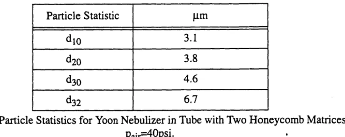
Table 3.3: Particle Statistics for Yoon Nebulizer in Tube with Two
Honeycomb Matrices; Pair=40psi ...50
Table 3.4: Particle Statistics for Yoon Nebulizer in Tube with a 4.5cm
Impaction Disk and a Honeycomb Matrix; Pair=
8 0psi ...50
Table 3.5: Particle Statistics for Yoon Nebulizer with a 5.1cm Impaction Disk ...51
Table 3.6: Spinning Disk Spray Characteristics, Q=0.65ml/s. with Surfactant ...58
Table 3.7: Spinning Disk Spray Characteristics, Q=O.Sml/s. with Surfactant ... 58
Table 3.8: Spinning Disk Spray Characteristics, Q=1.25ml/s. with Surfactant ...60
Table 3.9: Array Generator Particle Statistics (I) ... 64
Table 3.10: Array Generator Particle Statistics (II) ...65
Table 3.11: Array Generator Aerosol Fluid ...65
Table 4.1: Comparison of Track 3 and Track 2 Velocity Response Data ...99
Table 5. 1: T-Step Reattachment Length as a Function of U and hs... 146
Table A. 1: Modified Contraction Polyethylene Sheet Measurements ... ...250
Table A.2: Modified Contraction Insert Dimensions ...251
Table
.
1: Mean d Statistics for Externally Mounted SprayVector Atomizers...257
Table D.2: Oil Particle Mean dp Statistics ... 258
Table D.3: Comparison of NIST-certified Monodisperse PSL Spheres
to PDPA Measurements ...
.
...
26...261
Table E. 1: Mean dp Statistics in the Fully-Developed Region of
Channel Flow Experiments .
...
274
Nomenclature
A Constant in expression describing the decay of grid turbulence; a constant for the reflection of gas molecules from a particle
b Coefficient in particle drag expression when r-l
Cd
Concentration of fluorescein salt dye
D Spinning disc diameter
Dj
Diameter of VOAG jet
Dh
Channel hydraulic diameter
db
Diameter of laser beam
dp
Particle diameter
dstraw
Straw diameter used in straw bundle
d1o
Number mean particle diameter
d20
Area mean particle diameter
d30 Volume mean particle diameter
d32
Sauter mean particle diameter
E
Molar absorptivity of fluorescein dye
Fm Particle drag
fb
Natural frequency of jet breakup
fd
Driving frequency of jet
h Test section height
hp
Protrusion height
hs Step height I Light Intensity
If
Light absorbed by fluorescein
Io
Laser Intensity
J
Deposition rate
K
Film thickness equation coefficient
KD Deposition Velocity
1
Mean free path of carrier fluid
ii
Stop distance of aerosol
M
Biplane grid mesh size
N
Number count of aerosols in a distribution
ND
Number density of aerosols
n
Exponent describing the decay of grid turbulence; Spinning disk rotation
rate
nf
Number of fringes
Q Volume feed rate to spinning disk; constant in expression for particle drag
when r-l
Qf Volume rate of aerosol production
r
Aerosol radius; spinning disk radius
r
Mean aerosol radius
t
Deposition film thickness
S
Span parameter of spray monodispersity
t Deposited film thickness
tr
Deposition run time
U Mean flow velocity
us
Friction velocity
u'
Flow Root Mean-Squared (RMS) velocity
V
Deposition velocity
V+ Deposition velocity in viscous units Vj Jet velocity of VOAG.
Vp Particle instantaneous velocity
vd
Deposition velocity
v'
Particle RMS velocity; fluid RMS velocity normal to a surface
w Tunnel width
w'
Transverse flutuating velocity component
Xf
PDPA fringe spacing
x
Streamwise coordinate
Xr Mean reattachment length
x
0Virtual origin of homogeneous flow field
y Vertical coordinate normal to a horizontal surface
y+
Distance from a wall in viscous units
Ys
Splitter plate thickness
Yt Half-tunnel height (= (h - ys)/2)
z
Longitudinal coordinate
Rec Reynolds Number based on channel hydlraulic diameter
Rep
Reynolds Number based on particle diameter
Res Reynolds Number based on step height
Stk
Stokes Number
ca
Logarythm of the root-mean squared variation of particle diameter
F
Vorticity of secondary flow
A
5 Boundary layer thickness; channel flow half-height
Sf
Deposited film thickness
St Fringe crossing time intervall 0 Angle of PDPA configuration E Turbulent dissipation rate
Ag Integral scale of turbulence
X
Wavelength of jet disturbance; laser emission wavelength
?,opt
Optimum Wavelength of jet disturbance
gu
Viscosity of air
f Viscosity of aerosol fluid
v
Kinematic viscosity of air; Poisson's ratio
p
Density of air
pp
Densitv of aerosol
G Surface tension of fluid
oC RMS velocity fluctuation measured by PDPA
cOg
Degree of spray monodispersity for a log-normal distribution
GCM RMS velocity fluctuation due to long-term U drift Op RMS PDPA velocity error
Radial stress
oy Yield strength of material
xr
Particle relaxation time
Tf Characteristic flow time scale
tk
Kolmogorov time scale
TM
Characteristic time scale of integral length scale
Tp
Particle time scale and particle relaxation time
x+
Dimensionless particle relaxation time
tr
Reattachment Time Scale
Chapter 1 INTRODUCTION
Enhanced deposition rates occur in a secondary flow when an entrained particle strays
from the flow streamline and impacts a surface. A particle with little inertia tends to follow
the flow exactly and must rely upon non-impaction mechanisms (i.e.diffusional,
thermo-phoretic, and gravitational settling) to deposit because the flow structure does not intercept
the wall. On the other hand, more inertial particles will stray further from flow structures because they react more slowly to the flow. Moderately inertial aerosols, aerosols that exhibit some slip between the particle and the flow, behave in a regime between the two
and deposition rates would appear to be governed by how accurately the particles trace the
flow, or in other words, how precisely the velocity response of the aerosol mimics that of
the flow. Experimental measurements of deposition rate behind a flow obstruction (Kim et
al., 1984) indicate that deposition rates can be greatly augmented by a secondary flow
structure, while measurements of particle dispersion behind a backward-facing step (Ruck
and Mikiola, 1988) suggest that heightened deposition results from the particles entering
the secondary flow, deviating from the eddy and impacting the wall. In spite of the much
higher deposition rates reported in secondary flows, aerosol interaction with secondary
flow structures has not received much attention. The primary goal of this thesis is to
exper-imentally elucidate the deposition behavior of moderately inertial aerosols in secondary
1.1 The Contexts of Aerosol Deposition
The dispersion and deposition of aerosols occurs in numerous engineering
applica-tions related to the secondary flow described above. Aerosols have been implicated in the
erosion of metal surfaces (Smeltzer et al., 1969) and thrust nozzles (Bailey et al., 1961).
Tabakoff et al. (1991) discuss how the dust, salt and sand particles inhaled by gas turbine engines impact upon the turbine blades and wreak havoc upon the performance, endurance and reliability of the turbines. Aerosols in coal combustors accumulate on the surfaces of
heat exchanger tube bundles, fouling the surface and degrading heat exchanger efficiency
(Zhang et al., 1992).
Fine coal particles can dramatically erode surfaces of fluidized bed coal combustors.
Many investigators note that erosion is particularly extreme in regions where the
particle-laden flow passes over an object in the flow, such as a heat exchanger rod, welding seam, discontinuity in a wall, etc. (Johnk and Wietzke 1989, Bixler 1989, Miller 1989, Elsner
and Friedman 1989). In each instance, augmented erosion coincides with the existence of
a secondary flow: the alternating vortices shed off a heat exchanger rod or the separating-reattaching flow fore and/or aft of a step such as a weld seam. Humphrey (1990,1993) has
provided comprehensive reviews of the role of impacting particles in surface erosion.
The transport and subsequent deposition of toxic and carcinogenic particulates in the
lung is a related problem area. Pollutants such as cigarette smoke are inhaled and deposit
in the tracheobronchial tract; the spatial distribution of deposition within the lungs of
par-ticles of a given size is of primary interest in assessing the toxic potential of specific
pol-lutants. If the regions of highest deposition rate can be identified, therapeutic aerosols
could be targeted to the high-risk regions. Towards this end, deposition studies in human lung casts (Schlesinger et. al. 1977) have been performed. They conclusively demonstrate
that deposition rates of particles between approximately 0.1 and 3gm near lung
bifurca-tions (branchings) are much greater than in the straight passages. Earlier studies
(Auer-bach et al. 1961) found that the highest incidence of primary lung carcinomas are near the
bifurcations, and it is generally believed that increased particle deposition in specific areas of the lung caused some types of cancer. To explain such findings in terms of the fluid flow
within the lungs, Schlesinger et al. attributed the increase in deposition rate to the
impac-tion of inertial aerosols that fail to navigate the streamwise curvature present at
bifurca-tions.
Experimental simulation of a lung bifurcation by Jan et al. (1989) highlighted the
vig-orous secondary flows occurring at a bifurcation. Similarly, Kim (1984) measured the
deposition rate of moderately inertial aerosols behind an obstruction in a pipe flow
-representative of a partially obstructed lung bronchus - and discovered that deposition in
the reattachment zone was almost one hundred times that in unobstructed flow. He cited
the presence of the strong secondary flow behind the step as the reason for the augmented
deposition rate. Secondary flows are also usually present in curved tubes, such as
bron-chial airways and pipe elbows.
Ultra-fine aerosol deposition (dp = 0.01 - 0.5 m, say) studies provide further evidence
of elevated higher deposition rates in secondary flows. Studies at lung bifurcations
per-formed with ultra-fine aerosols found that deposition rates were more than twice as great
at those predicted by a unidirectional-flow diffusional theory (Cohen and Asgharian
(1990), Cohen et al. (1990)). Feng (1993), however, evaluated ultra-fine aerosol deposi-tion at various posideposi-tions behind a forward-backward facing step using a novel
transmis-sion electron microscopy (TEM) technique, finding lower deposition rates in the region of
1.2 Overview of Aerosol Dispersion
The fundamental issue of how closely a particle of a given inertia follows a flow
hav-ing a characteristic timescale 'rf, in addition to strongly influenchav-ing aerosol deposition
rates in turbulent (e.g. Maxey, 1987 and Hjelmfelt and Mocros, 1966) and secondary
flows, also bears upon the validity of Laser Doppler Anemometry (LDA) or Particle
Image Velocimetry (PIV). To apply LDA, the flow is seeded with particles and the LDA
apparatus measures the velocity of the particles; it is assumed that the particles accurately
represent the behavior of the flow and move approximately at the velocity of the flow. In
reality, particle behavior may not accurately portray the fluctuating velocity of the fluid,
since the inertia of a particle may prevent it from following all scales of the flow. A
parti-cle that would allow accurate measurement of the velocity field using LDA would have at
least three characteristics. First, the particle would be much smaller that the length scale of
an eddy, so that the particle itself would not create a turbulent flow field. Second, the parti-cle must have a timescale T that is much less than the smallest time-scale of the flow to
insure that the particle, despite its inertia, will be able to trace the smallest swirling
motions of the flow. Third, the mass loadings of the particles would be small enough so
that it did not damp the flow field turbulence (Hestroni, 1989) or alter the momentum of
the flow field.
1.3 The Essential Problem
This thesis describes a series of experiments designed to investigate several aspects of
aerosi dispersion and deposition in secondary flows. Aerosols encompassing a wide
wind tunnel (see Child, 1992). First, velocity response experiments are conducted to investigate the particle-fluid interaction for particles encompassing a vast range of particle
inertia in the approximately homogeneous turbulence developing behind a bi-plane grid.
Second, the deposition rates of particles are studied in the recirculating secondary flow behind a T-step. Particle deposition rates are then scaled with turbulent and secondary
flow timescales (e.g. the eddy turnover time) to determine whether the turbulent or
sec-ondary flow controls particle deposition behavior.
A study of aerosol deposition in secondary flows, however, could not be completed
without addressing several integral issues. When this project was begun, a suitable facility
for studying aerosol deposition did not exist in the Heat Transfer Lab; neither did a safe
technique for accurately quantifying local deposition rates. Chapter 2, "Instrumentation,
describes the aerosol wind-tunnel facility and recent improvements, the Laser-Induced
Fluorescence system (LIF) used to measure deposition rates, and the other measurement
techniques used during the course of this thesis. A crucial facet of performing aerosol
research is selecting an appropriate aerosol generation technique. Chapter 3,. "Aerosol
Generation," explains the pros and cons of several methods of aerosol production
consid-ered for experiments, operational performance and details of the generators tested, and the
array generator is selected for the aerosol deposition experiments.
As discussed earlier, the physics of aerosol deposition are directly related to the
ten-dency of the aerosols to follow the flow. "Particle Velocity-Response Experiments",
Chap-ter 4, reviews past models and investigations of particle dispersion, and the detailed
particle velocity-response experiments carried out to study the interaction of particles with
turbulent flow structures. The Aerometrics Phase-Doppler Particle Analyzer (PDPA)
flow deposition experiments, and Chapter 4 also contains a significant assessment of the
validity of the PDPA fluctuating velocity measurements.
Construction of the aerosol wind-tunnel facility, development of the experimental
methods, selecting the appropriate aerosol generation technique, and investigation of
par-ticle-turbulence interaction collectively stand as an essential prelude to studying particle
deposition in secondary flows. Chapter 5, "Deposition in Secondary Flow". first surveys
the deposition literature and then describes the present particle deposition results in the
secondary flow behind a T-step. The aerosol deposition rates in the recirculating region (i.e. the secondary flow) are compared to those of a turbulent boundary layer. In addition,
appropriate time scales for particle deposition in the secondary flow and the
approxi-mately plane mixing layer downstream of the recirculation are selected.
Chapter 2 Instrumentation
This chapter describes the aerosol wind-tunnel facility and the measurement
tech-niques used to measure aerosol deposition. First, I present the new and elongated
wind-tunnel made possible by the lab renovations in the summer of 1992, including the
modi-fied contraction. Second, I detail the application of hot-wire anemometry, to measure gas
phase velocities, and phase Doppler anemometry, to obtain simultaneous particle diameter
and velocity measurements. Finally, I discuss potential deposition measurement
tech-niques and their limitations, followed by an explanation of the Laser-Induced
Fluores-cence (LIF) technique developed to measure aerosol deposition for this thesis.
2.1 Aerosol Wind-Tunnel Facility
The Heat and Mass Transfer Lab Aerosol Wind Tunnel was originally constructed in
the summer of 1991 by Child, Colmenares, and Roth (see Child, 1992). Numerous
improvements have been made to the tunnel since the initial fabrication; the current tunnel is shown in Figure 2.1. The tunnel is a suction design through which flow is induced by a
0.75 horsepower blower located at the outlet. Air enters the tunnel through a straw bundle
(dstraw = 0.40 cm) bounded on both sides by 24-mesh wire screens. The bundle effectively
removes large swirling structures that may arise at the entrance and also creates a uniform
flow field across the section. Two additional 20-mesh screens further damp the turbulence.
In the injection section, an aerosol generator seeds the flow with micron-sized water
aero-sols which pass into the settling section where the turbulence created by the atomizers
decays before entering a 20:1 area ratio contraction. The five-foot long test section has a
variable-pitch roof to permit elimination of the streamwise pressure gradient. A 3/4
horse-power vane-axial blower creates freestream velocities of up to 13 m/s in the test section. The initial assessments of the tunnel (see Child, 1992, and Colmenares, 1992) did not
show any evidence of separation of the flow in the contraction. However, the author
per-formed hot-wire anemometer measurements of the tunnel that found thick regions (almost
7.5 cm) of bursting activity on both the top and bottom of the entrance to the test section.
Measurements at the rear of the section demonstrated that the turbulent layer had grown to
span the entire height of the test section. It is not known whether the turbulent layer was
present in the test section before November 1992. The wind tunnel had been disassembled
during the summer of 1992 to accommodate laboratory renovations and the settling
sec-tion was appended to the tunnel subsequent to those renovasec-tions and these changes in
tun-nel geometry may have altered the tuntun-nel flow. To determine the cause and location of the
turbulent wall layer, titanium dioxide visualization was used. TiCl
4liquid was injected
with a syringe just upstream of the mouth of the contraction. The TiC1
4reacted readily
with the moisture in the air to form very small (0.02-1.0 gm) TiO2particles (see Appendix C and Feng, 1994) which readily follow the streamlines of the flow. Flow visualization
revealed a sizeable vortex at the mouth of the contraction and intermittent break-off and
convection of the vortex into the contraction. Thus, the growing shear layer in the test
sec-tion was attributed to the erratic behavior of the flow at the base of the contracsec-tion. This
behavior appeared to result from boundary layer separation owing to an adverse local
pressure gradient at the mouth of the contraction.
Initially, coarse (30-grit) sandpaper was affixed to the surface of the contraction to trip the flow and attempt to prevent flow separation. Unfortunately, the flow separation remained and the original contraction had to be redesigned. Several contraction
geome-the wall. Ultimately, an elongated contraction shape that greatly smoogeome-thed he mouth of the contraction was selected (see Appendix D for the coordinates) and when installed on all four sides of the tunnel, 5=1.2-1.6 cm on the bottom of the tunnel.
Boundary layer thickness measurements were used to evaluate the performance of the
redesigned contraction. These measurements could not be made at the top or sides of the
tunnel with the hot-wire probe, owing to probe spatial constraints. Along the bottom wall,
at x=137cm downstream of the test section entrance (15.2cm from the end of the test
sec-tion), 5 had grown to 3.2-3.8cm, consistent with the growth rate of a turbulent boundary
layer (Schlichting, 1987) having its virtual origin in the throat of the contraction. The
redesign clearly alleviated the separation problem. The vertical velocity gradient that
Childs (1992) noted in his assessment of the original tunnel performance also ceased to
exist. '
The final contraction shape was made using inserts constructed out of 0.76mm thick
polyethylene sheet mounted with RTV Silicone Sealant onto polystyrene blocks cut to the
desired contraction shape; RTV silicone sealant also affixed the polystyrene blocks to the
four sides of the tunnel. Duct tape held the front and back lips of the polyethylene sheet in
place and also mated the edges where four sheets intersected.
In order to gain access to the interior for altering the contraction shape, a 73cm high by
71cm wide access door was cut in the settling section near the beginning of the
contrac-tion. Efforts were made to insure that the wall discontinuity generated by the door did not
upset the flow; there were no indications that the door did significantly disturb the flow in
the test section (i.e. no evidence of flow separation). An estimate of the protrusion height,
hp, required to induce a turbulent transition can be made using Tani's (1969) step criterion:
hpU
2h> 825 (2.1)
Taking U in the test section to be 10 m/s (a typical operating condition), U at the door is 0.5 m/s, requiring hp to be higher than 2.5cm to effect a turbulent transition. In practice, hp was much less than one inch, indicating that the flow should not undergo transition at the door discontinuity.
Upon leaving the revamped contraction, the flow entered the new test section which has been elongated to 152cm. The roof was pinned at the front and can be pitched up at
angles of over 10 to counteract boundary layer growth and maintain a constant velocity in
the tunnel core. A 0.95cm wide slot extends from the front of the section to the rear to
per-mit access of hot-wire and pitot probes to the test section. Two foam rubber strips mounted
flush with the roof and centered on the instrumentation slot deform to accommodate the
probes and form a seal to prevent air from entering via the slot. A 12.7cm diameter plug at
the rear of the test section provided easy access to the rear of the test section.
2.2 Hot-Wire Anemometry
A TSI 1210 T1.5 hot-wire probe, mounted in a TSI probe support, was driven by a TSI
IFA-100, a constant-temperature anemometer bridge circuit. The overheat ratio, OHR, is
the ratio of the hot probe resistance, Rh, to the cold probe resistance, R
c. Typically, an
overheat ratio of 1.8 was used:
RH
OHR = R (2.2)
Rc
The frequency response of the IFA bridge was optimized before tests per the IFA-100
1987 Instruction Manual; Fingerson and Freymuth (from Thermo-Systems, Inc., 1987)
report a post-optimization cut-off frequency of at least 96kHz, well above the frequencies
encountered in the present experiments. A Masscomp 5400 (with EF12M A/D boards)
cessing routines, an3.f and answ.f; the original code was composed by Kay Herbert and
the two codes are substanitally altered versions created by Kurt Roth. The bridge signal was low-pass filtered at 4kHz by a Precision Filters, Inc. Model 32-01-LP1; the low-pass filter is a six-pole, six-zero elliptic filter characterized by a O.ldB band pass ripple and a
roll-off of 80dB/octave.
The hot-wire was calibrated against a pitot-static probe (a MKS Baratron 398HC-0001 pressure transducer measured the differential pressure) in the tunnel. To obtain an accurate
calibration, the A/D hardware and software captured 80,000 hot-wire voltages at a sample
rate of 8kHz (to avoid aliasing) and averaged them. At least ten different velocity points
were used in each calibration, encompassing the anticipated operating velocity range of
the probe. A fourth-order least-squares curve fit, consistent with King's Law, related mean
velocity to voltage.
2.2.1 A/D Discretization Error
The discretization error of the 12-bit A/D board (the EF12M) necessitated the use of
the two distinctly different programs. The EF12M accepts input voltages of +/- 10 volts.
Dividing this by the number of bits (2
12)yields the discretization of the incoming signal,
4.88mV. Thus, the EF12M digitizes each incoming voltage signal to an accuracy of
+/-2.44mV. Typical amplified hot-wire fluctuating voltages ranged from 0.2mV for the open
test section (very low turbulence levels) up to 20mv in the turbulent boundary layers of the
bottom wall. Thus, if the raw hot-wire signal of the open test section flow was acquired by
the EF12M, the A/D discretization error would be an order of magnitude greater than the
signal to be measured, resulting in incorrect turbulence intensities. Two approaches were taken to avoid A/D discretization errors. In the first case, program answ.f, the IFA signal
was split into two channels. The first was DC coupled. The second was AC coupled, low-pass filtered at 4kHz, and amplified by a factor of 100. Amplifying the AC component of
the hot-wire signal minimized discretization errors by making the signal an order of
mag-nitude greater than the discretization error for the smallest signals encountered. Answ.f
obtained the mean velocity by summing all of the incoming DC voltages and then dividing
by the number of samples to obtain a mean voltage. The AC voltages were added to the
mean and each data point was converted to a velocity using a fourth-order hot-wire
cali-bration equation.
Although the answ.f routine prevents A/D discretization errors, and effectively
acquires low-level signals, it does not accurately report higher turbulent intensities, such
as those found at the centerline of a turbulent air jet. A second data acquisition program,
an3.f, solved the problem by using only a DC voltage channel, low-pass filtered at 4kHz
and having a gain of 5. The increased gain helped to minimize discretization error,
espe-cially at higher turbulence intensities where the fluctuating signal was now greater than A/
D discretization. However, a discretization turbulence intensity of approximately 0.4%
still existed, rendering an3.f of limited utility for turbulence intensities of less than
one-percent. Thus, answ.f was used to quantify flows with turbulent intensities less than 1.0%,
and an3.f for higher turbulence intensities.
2.3 Phase-Doppler Particle Anemometry
The Phase Doppler Particle Analyzer (PDPA) is a laser doppler anemometer
manufac-tured by Aerometrics of Sunnyvale, CA that is capable of simultaneously measuring a
sin-gle component of particle velocity and particle diameter. Details of the PDPA operation
(1984) thoroughly describe PDPA theory. A velocity offset capability, produced by a rotat-ing diffraction gratrotat-ing that shifts the frequency of one of the laser beams, enables mea-surement of negative particle velocities such as those present in reversing flows.
The transmitter and receiver of the PDPA were mounted on a rigid Newport laser
plat-form, maintaining a consistent alignment of the transmitter and receiver. The platform was
mounted on stainless steel rails oriented parallel to the flow, which in turn were attached to
a Unistrut table used by Simo and Lienhard (1991), Colmenares (1992), and Child (1992).
A pressurized air cylinder allows rough positioning in the vertical y-direction.
Unfortu-nately, after much exposure to water aerosols the table had become quite warped and much effort was required to maintain the table in a plane parallel to the ground. Further-more, the cylinder slowly leaked, causing the height and orientation of the table to drift
with time. During this work. the laser platform was re-mounted on a Rambaudi machining
bed in the fall of 1993. The machining bed, which is itself mounted on a 0.64cm steel plate on a pallet roller, provides much improved stability and allows positioning in the y (verti-cal) and z (horizontally normal to the flow) directions to a precision of +/- 0.0lmm.
The PDPA measures particle velocities in the same manner as an LDA. Two laser
beams, each with a power of 5mW and a diameter of 133 gxm pass through the 200mm
transmitter lens and converge, intercepting at the focal point to form the probe volume.
The probe volume consists of alternating bands of constructive and destructive
interfer-ence (i.e. bands of high intensity and much lower intensity) of the light waves known as
fringes, and the fringe spacing is determined by the angle of the beam interception. As the
particles pass through the bands of the probe volume, they scatter the light of variable
intensity from the alternating bands: this is the doppler burst. The 495mm receiving lens collects refracted light scattered off the particles in the probe volume which it focuses upon three photomultiplier tubes (PMT) oriented in the streamwise direction. The PMT
amplifies the light signal and converts photons to a current in successive stages, and its gain is governed by the PMT voltage, VpMT, selected by the user. The raw voltage signal
from the PMT (representing scattered light intensity) has a high frequency component
rep-resenting the interference fringes and a low frequency component, or pedestal, that results
from the Gaussian distribution of fringe intensity across the probe volume. Velocity
mea-surements are derived solely front the high frequency portion of the signal, so the pedestal
is removed during processing by a high-pass filter. The PDPA coprocessor electronically
conditions the signal and ultimately counts the time, ft, it takes for a pre-determined
num-ber of zero crossings, nf, to occur. Because the fringe spacing, Xf, is known, the particle
velocity may be easily calculated:
vp t (2.3)
VP 8 t
Particle diameter measurements are obtained by studying the phase difference of the
signal at three different PMTs. The light waves pass through the particle and are bent by
the differing index of refraction of the particle. The longer the light wave remains in the
particle the farther it propagates in the new direction; the greater the particle diameter the
greater the "bending" of the light. The phase lag that exists between the different PMTs
due to the light bending and the spacing of the PMTs can be expressed using Mie
scatter-ing theory in terms of the index of refraction of the particle and the medium, the geometry
of the PMTs relative to the probe volume, and the particle diameter (see Bachalo and
Hauser (1984) for a derivation). Because all variables except the particle diameter are known, the phase shift between the detectors yields the particle diameter. The three PMTs
also provide a check on particle diameter measurement. For each burst detected, the PDPA
software compares the particle diameter measurements between the first and second PMTs
with that obtained between the first and third PMTs. If the two estimates of particle
diam-eter differ, the software rejects the burst and ignores the measurement.
In all tests performed, the PDPA operated in the forward scatter configuration with the
receiver aligned at 0=30
°with respect to the transmitter. A larger angle, such as 0=60
°,
would provide improved dp resolution for smaller particles by increasing the magnitude of
the phase-shift between the PMTs. However, the amount of light reaching the PMTs
decreases as 0 becomes greater, reducing the signal intensity. When 0<30
°, the component
of reflected light increases substantially, increasing optical noise and producing more
fre-quent measurement errors. Thus, operating at 0=300 represents a reasonable compromise to obtain high signal quality over a range of particle diameters.
The PDPA configuration may also be optimized to look at a specific range of particle
diameters by selecting one of three available transmitter beam spacings, or "tracks". The
PDPA can quantify particles over a range including particles 35 times larger than the
smallest diameter selected, e.g. dp=1.4-50 gm. Table 2.1 presents the characteristics of the
three grating tracks for the lenses used (Aerometrics, 1987):
Characteristic
Track 1
Track 2
Track 3
dp range, gm
0.7-105
1.4-205
2.8-410
Nf 26 13 7
Beam Diameter, 133 133 133
Table 2.1: Characteristics of the PDPA Tracks.
Proper PDPA alignment is essential to obtaining meaningful velocity and diameter
measurements, as well as optimal data acquisition rates. Before beginning each
correct probe volume was created. During tests, observations made through the side por-tals of the receiver confirmed that the probe volume was centered on the PMT slit and that the beam interception remained true. The quality of the unfiltered and filter doppler bursts was monitored on a 20MHz Phillips analog oscilloscope during every run. The quality of the doppler bursts became particularly helpful in evaluating how particle deposition on the side wall affected measurements. When signal quality was observed to have significantly
declined, the walls were either air-dried or hand-cleaned with paper towel.
2.4 Deposition Measurement
Particle deposition on a surface can be extremely difficult to quantify. In the past, a
num-ber of techniques have been used, including dye-washing techniques (Kim 1984, Ball and
Mitchell, 1992), radioactive counting (Sweeney et al. 1990), fluorescent tracers (Zeltner
et al. 1991), and attenuation of a light source by the deposited material (Lee and Hanratty
1988). Farmer (1969) burned a ribbon of magnesium inside of a tube, coating the inside of
the tube with a fine layer of magnesium oxide where the depositing particles left a particle
diameter-calibrated imprint. He quantified deposition rate by counting and sizing the
imprints with a magnifying glass. Many of these methods are simply unacceptable for our
purposes, as they either do not provide the spatial resolution necessary for an accurate
cor-relation between deposition and the flow patterns (dye-washing techniques), would
dam-age the wind-tunnel environment (MgO) or are difficult to implement safely (radioactive
tracing). In addition, liquid aerosols tend to evaporate and may spread upon impaction, forming thin layers that smooth out local variations in the deposition rate.