Design of a 460 GHz second harmonic gyrotron oscillator for use in dynamic nuclear polarization

Design of a 460 GHz Second Harmonic Gyrotron

Oscillator for use in Dynamic Nuclear Polarization

by

Melissa K. Hornstein

B.S.,

Electrical and Computer Engineering (1999)

Rutgers University

Submitted to the Department of Electrical Engineering and Computer

Science

in partial fulfillment of the requirements for the degree of

Master of Science in Electrical Engineering and Computer Science

at the

MASSACHUSETTS INSTITUTE OF TECHNOLOGY

September 2001

@

Massachusetts Institute of Technology 2001. All right

OF TECHSNOLOGY

BAR

NOV 01 2001

LIBRARIES

A uthor ... ... .... ... ... E

Department of Electrical Engineering and Computer Science

August 24, 2001

Certified by...

Richard J. Temkin

Senior Research Scientist, Department of Physics

Supervisor

Accepted by ... ...

Arthur C. Smith

Chairman, Department Committee on Graduate Students

Design of a 460 GHz Second Harmonic Gyrotron Oscillator

for use in Dynamic Nuclear Polarization

by

Melissa K. Hornstein

Submitted to the Department of Electrical Engineering and Computer Science on August 24, 2001, in partial fulfillment of the

requirements for the degree of

Master of Science in Electrical Engineering and Computer Science

Abstract

Dynamic nuclear polarization (DNP) is a promising technique for sensitivity enhance-ment in the nuclear magnetic resonance (NMR) of biological solids. Resolution in the NMR experiment is related to the strength of the static magnetic field. For that rea-son, high resolution DNP NMR requires a reliable millimeter/sub-millmeter coherent source, such as a gyrotron, operating at high power levels. In this work we report the design of a gyrotron oscillator for continuous-wave operation in the TE06 mode at 460 GHz at a power level of up to 50 W to provide microwave power to a 16.4 T 700 MHz NMR system and 460 GHz EPR/DNP unit. The gyrotron design is closely modeled on a previous successful design of a 25 W, 250 GHz CW gyrotron oscilla-tor. The present design will operate at second harmonic of the cyclotron frequency, w ~ 2w,. Second harmonic operation requires careful analysis in order to optimize the oscillator design under conditions of moderate gain, high ohmic loss, and competition from fundamental (w ~ w,) modes. In addition, an internal mode converter will be used. The output radiation will propagate through a window and perpendicular to the magnetic field through a cross-bore pipe in the magnet. The radiation will then travel through a transmission line to arrive at the probe used for NMR experiments. In addition, the transmission line of a 140 GHz gyrotron oscillator currently operating in DNP-NMR experiments, including an external serpentine mode converter which converts the TEO, to TE11 mode, is analyzed experimentally and theoretically. Thesis Supervisor: Richard J. Temkin

Acknowledgments

This masterwork is exactly that: a work. Moreover, it flows from the wells of conti-nuity upon giants' shoulders much like a droplet, in hopes of becoming a splash. Let me now recount to you a passage from Kahlil Gibran's "The Prophet" [1].

You work that you may keep pace with the earth and the soul of the earth. For to be idle is to become a stranger unto the seasons, and to step out of life's procession, that marches in majesty and proud submission towards the infinite. When you work you are a flute through whose heart the whispering of the hours turns to music. Which of you would be a reed, dumb and silent, when all else sings together in unison? Always you have been told that work is a curse and a labor, a misfortune. But I say to you that when you work you fulfil a part of earth's furthest dream, assigned to you when that dream was born, And in keeping yourself with labor you are in truth loving life, And to love life through labor is to be intimate with life's inmost secret. ... Work is love made visible. And if you cannot work with love but only with distaste, it is better that you should leave your work and sit at the gate of the temple and take alms of those who work with joy. For if you bake bread with indifference, you bake a bitter bread that feeds but half man's hunger. And if you grudge the crushing of the grapes, your grudge distills a poison in the wine. And if you sing though as angels, and love not the singing, you muffle man's ears to the voices of the day and the voices of the night.

Many shoulders were scrambled upon in the completion of this work, like a tower of tumbling skydivers standing strongly in the four winds upon their imaginary frame-work that only they and Don Quixote can see. For it is the giants who must believe the existence of the windmill. And the rest of us to prove it. And would for we should never stop dreaming lest all should come crashing down? And who are those skyclimbers who support with their minds and hearts?

In impressionable and impressive times, both Sigrid McAfee and Evangelia Tzanakou (like ebb and flow) wove a seesaw hodgepodge patchwork girl into a yarn of her choos-ing. Thank you Professors for speaking with wisdom, steering with stories, and not looking up to count the countless pink hourglass sands fallen whilst we forgot the worries whisking past the open door.

In the uncertain days, Jagadishwar Sirigiri showed me his Lab when I was still known as a "Teaching Assistant". Ken Kreischer started me on this Work, and tried

to teach me all he knew in record time. Only I think my ears had a lot of wax in them. And thus Richard Temkin became my Mentor. Thank you, Rick, Ken, and Jags. And that was only the Beginning. Now I have come to know and depend on many more, as numerous as the Stars in a Night Lake:

Michael Shapiro Bob Griffin Jim Anderson Steve Korbly Vik Bajaj Melanie Rosay

the other Graduate Students Jeff Vieregg

Simplicious

Paul "Mr. Magnet" Thomas Catherine Fiore &

Amanda Hubbard

my Mother and my Father my Three Sisters

Toto (not the gyrotron), Oskar, & family

without whom a lot of Theoretical

Things worldwide would not be possible for inspiring me to have a Couch in my office my Officemate, for answering Stupid

Questions that ought'nt've been asked for his help on EGUN simulations for knowing alot about Chemistry for taking care of the Gyrotron for Reasons only they know for his work on the Controls for Library Things

for bringing meaning to the Result for the Women's Lunches

for for for

Much More Sisterly Things

the support given by Dogs & Family

And until the end, after thanking my Good Friends, some of whom I call Sisters and Brothers in Arms (don't scold me for not writing Your Names; there is a magic in the Unspoken!), should we awake to realize that we are but the dream of a mad knight errant, let the lesson be in not grudging the essence of our daily lives but in knowing the luck of oneday joining the ranks of the giants in the sky.

6

Contents

1 Introduction

2 Principles and Theory

2.1 Gyrotron theory . . . . 2.1.1 Electron beam . . . . 2.1.2 Principles of interaction between electrons and field 2.1.3 Non-linear theory . . . . 2.1.4 Second harmonic challenges . . . . 2.2 Nuclear magnetic resonance . . . . 2.2.1 Dynamic nuclear polarization . . . .

3 460 GHz Gyrotron Design 3.1 250 GHz gyrotron . . . . 3.2 Cavity design . . . . 3.2.1 NMR considerations . . 3.2.2 Second harmonic . . . . 3.3 Superconducting magnet . . . . 3.4 Electron gun . . . . 3.5 Quasi-optical transmission line . 3.5.1 Internal mode converter 3.5.2 Transmission line . . . . 3.6 Discussion . . . . 15 19 19 20 24 33 38 39 40 43 . . . . 4 5 . . . . 4 5 . . . . 4 6 . . . . 4 8 . . . . 5 3 . . . . 5 3 . . . . 5 5 . . . . 5 5 . . . . 5 6 . . . . 5 6

4 Transmission Line 59

4.1 Snake mode converter experiment . . . . 62

4.1.1 Setup . . . . 62

4.1.2 Radiation pattern measurements . . . . 63

4.1.3 Snake analysis . . . . 63

4.1.4 Mode conversion theory . . . . 73

4.2 Transmission line losses. . . . . 79

4.3 D iscussion . . . . 81

5 Conclusions 83

A Glossary 85

List of Figures

2-1 Magnetron injection gun with beam [2] . . . . 24 2-2 Uncoupled dispersion diagram showing the region of interaction

be-tween the waveguide modes, the beam, and beam harmonics [3] . . . 29 2-3 Gyrotron phase bunching: (a) initial condition, where the electrons are

uniformly distributed on a beamlet (b) new positions of the electrons immediately after the change in energy (c) formation of the electron bunch [4] . . . . 31 2-4 Quadrapole electric field for a second harmonic interaction [4] . . . . 33 2-5 Transverse efficiency contour yj (solid line) as a function of the

nor-malized field amplitude F and nornor-malized effective interaction length M for optimum detuning A (dashed line) and second harmonic n = 2 [5] 36 3-1 Schematic of the 460 GHz gyrotron for DNP . . . . 44 3-2 Cavity design and RF field profile . . . . 47 3-3 Chart of the TE mode indices up to vmp = 21 . . . . 50 3-4 Starting current for modes in the vicinity of the TE06 design mode,

with the design parameters of Table 3.2 . . . . 51 3-5 Normalized field amplitude versus beam radius for the TE06 mode . . 52 3-6 EGUN simulation . . . . 54 3-7 Schematic of the quasi-optical internal mode converter showing

3-8 Drawing of the internal mode converter (including launcher and mir-rors) indicating the paths of the electron and RF beams, and output w indow . . . . 58 4-1 (a) Schematic of the TEoi - TE11 snake mode converter, where a is

the waveguide radius, 6 is the perturbation, d is a period, and L is the total length (b) close-up of one period . . . . 60 4-2 Schematic of the 140 GHz transmission line . . . . 61 4-3 (a) Horizontal and (b) vertical polarizations of the gyrotron output at

z = 5.08 cm; normalized dB contour plot . . . . 64 4-4 Gyrotron output at z = 5.08 cm, (a) y = 0; (b) x = 0; the solid line

represents the total intensity, the dotted line the vertical polarization, and the dashed line the horizontal polarization . . . . 65 4-5 (a) Horizontal and (b) vertical polarizations of the snake output at z

= 5.08 cm; normalized dB contour plot . . . . 66 4-6 Snake output at z = 5.08 cm, (a) y = 0; (b) x = 0; the solid line

represents the total intensity, the dotted line the vertical polarization, and the dashed line the horizontal polarization . . . . 67 4-7 Sum of horizontal and vertical polariations at z = 5.08 cm of (a)

gy-rotron output; (b) snake output; normalized dB contour plot . . . . . 69 4-8 (a) TEoi and (b) TE₁₁ theoretically radiated at z = 5.08 cm;

normal-ized dB contour plot . . . . 70 4-9 (a) Horizontal and (b) vertical polarizations of TEoi intensity

theoret-ically radiated at z = 5.08 cm; normalized dB contour plot . . . . 71 4-10 (a) Horizontal and (b) vertical polarizations of TE11 intensity

theoret-ically radiated at z = 5.08 cm; normalized dB contour plot . . . . 72 4-11 Intensity of 60% TEoi and 40% TE11 (33.750) is shown for (a) vertical

and (b) horizontal polarizations; radiated at z = 5.08 cm; normalized dB contour plot . . . . 74

4-12 Intensity of 65% TEO, and 35% TE11 (-75") is shown for (a) vertical and (b) horizontal polarizations; radiated at z = 5.08 cm; normalized dB contour plot . . . . 75

List of Tables

1.1 Progress in DNP gyrotrons at MIT . . . . 17

3.1 Comparison of important 250 and 460 GHz gyrotron design parameters 45 3.2 Gyrotron cavity design parameters . . . . 46

3.3 Beam extraction parameters . . . . 46

3.4 Quasi-optical mode converter parameters . . . . 56

4.1 Inputs to the two-mode approach . . . . 77

4.2 Optimum two-mode approach snake parameters . . . . 78

4.3 Measured snake parameters . . . . 78

4.4 Conversion efficiency of the snake in the multi-mode approach . . . . 78

Chapter 1

Introduction

The gyrotron oscillator, sometimes referred to as the "electron cyclotron resonance maser") or "gyromonotron", is a high-power high-frequency source of coherent elec-tromagnetic radiation [7]. It is a fast-wave device, one of the latest additions to the microwave tube family, which can operate with efficiencies as high as 60% [8]. Gy-rotrons can operate throughout the microwave and millimeter-wave spectra, inching into the sub-millimeter-wave spectra.

In the microwave regime (3 - 30 GHz), conventional microwave tubes such as klystrons, traveling wave tubes (TWTs), and backward wave oscillators (BWOs), all slow-wave devices, are fierce competitors. The dimensions of the interaction struc-tures of these slow-wave devices scale down accordingly with increasing frequency of operation; their decreasing structure size intrinsically limits these devices to the microwave regime due to increasingly high power levels and ohmic heating concerns. Thus, the millimeter-wave band (30 - 300 GHz) witnesses the inherent dominance of gyrotrons in generating high power, supplanting the pre-eminence of the conventional microwave tubes.

In the sub-millimeter-wave regime (> 300 GHz), the need to operate at harmonics of the cyclotron frequency due to limitations of the superconducting solenoids that provide the magnetic field leave this range at a draw, perhaps acquiescing to free-electron-lasers (FELs) or still gyrotrons with a clever design [9]. This work endeavors to demonstrate that gyrotrons can also occupy this burgeoning niche.

The gyrotron is a source of high power coherent radiation. It consists of a mag-netron injection gun, which generates an annular electron beam which is focussed into an open cavity resonator along an axial magnetic field, created by a superconducting magnet. In the cavity, the RF field interacts with the cyclotron motion of the elec-trons in the beam and converts the transverse kinetic energy into an RF beam which may then be internally converted into a Gaussian beam. The spent electron beam leaves the cavity and propagates to the collector where it is collected.

The development of gyrotrons has split in two main directions. High power milime-ter wave gyrotrons are needed as the power sources of electron cyclotron heating (ECH) of plasmas, electron cyclotron current drive of tokamaks [10], radar [11], and for ceramic sintering [12]. Medium power millimeter to submillimeter wave gyrotrons are required for plasma scattering measurements [13], and more recently electron spin resonance (ESR) experiments [14] and nuclear magnetic resonance (NMR) signal en-hancement by dynamic nuclear polarization (DNP) [15, 16, 17, 18, 19, 20, 21]. This paper will discuss the design of a gyrotron for the latter purpose.

Due to small nuclear Zeeman energy splittings and correspondingly small bulk magnetization at thermal equilibrium, NMR spectroscopy is plagued by low sensitiv-ity. Relaxation processes in the solid state further compromise these experiments, with the result that solid state NMR experiments have two or three orders of mag-nitude lower sensitivity in time than comparable experiments in the solution state. Dynamic nuclear polarization is a technique for sensitivity enhancement in these stud-ies. Previously, its application has been restricted to low magnetic fields, a regime in which the resolution of typical NMR spectra is not sufficient for structure determi-nation of large macromolecules. This restriction was due mostly to the lack of robust millimeter wave sources required for the DNP experiment at high fields; available sources relied on slow-wave structures which are fragile and cannot support sustained operation at the power levels required for DNP experiments. The cyclotron resonance maser, or gyrotron, is a fast-wave, millimeter/sub-millimeter wavelength device de-veloped for high power (megawatt-range) plasma heating. Because it is a fast-wave device, it is not dimensionally constrained to the order of a wavelength, and it can

Table 1.1: Progress in DNP gyrotrons at MIT Year Frequency Cyclotron

[GHz] Harmonic

1990 140 1

1998 250 1

2001 460 2

be easily scaled to the lower powers and higher duty cycles required for DNP.

In this work, we present the design of a high power second harmonic gyrotron oscil-lator for use in dynamic nuclear polarization experiments at 460 GHz in conjunction with a 700 MHz, 16.4 T NMR system. The design is based upon a continuous-wave 250 GHz gyrotron oscillator which is already used in DNP experiments. A DNP-NMR spectrometer operating with a 140 GHz gyrotron has also been successfully implemented and achieved signal enhancements.

Some relevant theory of gyrotrons and DNP is presented in Chapter 2. Chapter 3 describes the design parameters and simulations of the 460 GHz gyrotron in detail. A related experiment of the transmission line, including a snake mode converter, of a 140 GHz DNP-gyrotron will be presented in Chapter 4. Finally, chapter 5 contains some concluding remarks.

Chapter 2

Principles and Theory

2.1

Gyrotron theory

This is merely an introduction to relevant topics in gyrotron, nuclear magnetic reso-nance, and dynamic nuclear polarization theory. A more complete description of gy-rotron theory can be found through various references in the bibliography [7, 8, 9, 22]. A useful introduction to NMR theory can be found in [23]. This chapter presents some of the more immediately useful gyrotron equations, most importantly including a dis-cussion of the mechanism through which the electron beam couples with the RF field

and transfers its energy to the resonant cavity mode.

The gyrotron, as with all microwave sources, is based on the conversion of electron beam energy into radiation using a resonant structure. An annular electron beam is produced by a magnetron injection gun and travels through a resonant cavity, located at the center of the superconducting magnet. The magnetic field causes the electrons to gyrate and thus emit radiation. If the magnetic field and cavity are tuned to match the beam parameters, the radiation will couple into a resonant cavity TE mode. When the interaction is completed, the spent beam leaves the cavity and propagates to the collector. The microwaves are transmitted from the cavity to a mode converter, where they are transformed into a Gaussian beam that then exits the gyrotron through a vacuum window. Past the window, the beam can then be propagated down a transmission line, usually a cylindrical waveguide, to its place of

use.

2.1.1

Electron beam

First, let's begin from the electron beam. The electron beam is generated by an electron gun at the cathode and accelerated towards the anode. In the region between the cathode and the anode, the electric and magnetic fields are more or less constant, with the electric fields lines and magnetic field lines perpendicular to each other. The electrons have a constant E x B drift velocity VIK given by

VIK B2 (2.1)

ELK

VIK = (2.2)

BK

As the electrons reach the end of the cathode-anode region, the electric field lines change from mostly perpendicular to parallel to the magnetic field lines. This change in ELK at the cathode over a gyro-period implies a non-adiabatic transition.

When the electrons acquire a velocity perpendicular to the axial magnetic field, they experience a Lorentz force,

F = e x BO (2.3)

c

resulting in the creation of a circular motion with angular frequency eB0

Wc = (2.4)

my

where

y= - (2.5)

is the relativistic mass factor. The result of the superposition of the circular motion on axial motion is a helically gyrating trajectory about a fixed guiding center, where

the radius of the path, the Larmor radius,

V1L

rL = - (2.6)

wc

is small compared to the radius of the beam, so that the beam remains annular in its propagation.

The magnetic field at the cathode, BK, increases with increasing axial distance until the cavity where it reaches its maximum value of B0. The emitted electrons follow the magnetic field lines to the cavity where the interaction with the RF field takes place and microwave radiation is generated. In this region, the electromagnetic fields vary slowly in comparison with a gyro-period, hence the adiabatic electron magnetic moment pa, where m is the electron's mass and v is its velocity, given by

1 M2

Pa = (2.7)

is conserved.

The conservation of Pa allows the perpendicular velocity of the beam in the cavity, v10 to be written in terms of the perpendicular velocity of the beam in the cathode

VIK, as

B0

V±O = VIK B (2.8)

BK

where BO/BK is known as the magnetic compression of the beam. Combining Eqs. 2.2 and 2.8 gives

ElK B0

V = BK B (2.9)

BK BK

If v10 < vo then the beam will reach the cavity with the perpendicular velocity defined above. However if v10 > vo, then the electrons will be reflected back toward the cathode, causing the electrons to become trapped, leading to charge buildup and arcing. The total velocity vo is given by the kinetic energy conservation equation,

1 m2 (2.11)

= (v o ,me (2.12)

where me is the mass of an electron, VK is the cathode voltage, and Vpe is the space charge voltage depression.

The beam radius, r, is determined by the invariance of magnetic flux,

OD = 7rr2B = constant. (2.13)

With a beam radius rK and magnetic field BK at the cathode, we find that the beam radius in the cavity, reo (with a cavity magnetic field Bo) is

reo = rK BK (2.14)

B0 Adiabatic theory

"Adiabatic" is defined as "occurring without loss or gain". The adiabatic approxi-mation describes the basic equations of the electron beam. Adiabatic theory requires that the electron magnetic moment pa of Eq. 2.7 be held constant.

However, our approximation excludes the region of the gun, since the approxi-mation is only valid if the scale length of the variations of the electric and magnetic fields are small compared to the electron gyro-motion.

&2_{{B, E} {B, E} (.5} 02fB j

<

f _j (2.15) az2 2 &{B, E} {B, E} < (2.16)

az

zL

where zL is the axial distance that the electron propagates during one cyclotron period.

Therefore the adiabatic theory does not provide accurate results for the transverse velocity of the electrons in the vicinity of the gun.

Self-consistent simulations

To follow the trajectories of the electrons in this locality, numerical simulations are often used to more accurately calculate this information. An example of one of these codes, a modified version of the electron optics code EGUN developed by Herrmanns-feldt at Stanford Linear Accelerator [24], was used to design the electron gun for the present gyrotron design. The beam characteristics generated by this code have been demonstrated to have superior accuracy to the theoretical calculations approximated from adiabatic theory.

As inputs, the code needs the surface geometry of the cathode, anode, gun, and gyrotron tube (as far as will need to be modeled) and also the B-field of the magnet. The code in turn calculates the ratio of transverse to axial velocity a, the spreads in both the transverse and axial velocities, the beam radius and width, and the trajectories of the electrons being simulated. The code accounts for space charge, self magnetic fields, and relativistic effects. The program is a 2 1/2 dimension code; the fields are 2-dimensional while the particle trajectories are 3-dimensional.

To solve for the electron trajectories, first Poisson's equation (with no space charge) is solved by the method of finite differences, then potentials are differen-tiated from the electrostatic fields. Magnetic fields are specified externally, and the beam self magnetic field and electron trajectories are calculated for the E and B-fields. Poisson's equation is then solved again with inclusion of the beam charge and the electron trajectories are re-solved accounting for space charge. The iterations persist until they reach a convergence and provide self-consistent results.

The EGUN code can be used to elegantly design an electron gun, or to merely propagate the electron beam to assist in the design of the device.

Magnetron Injection Guns

The source of the annular electron beam used in gyrotrons, this "electron gun" that we have assumed until now, is usually a magnetron injection gun (MIG). A typical triode MIG configuration, a single cathode and two anodes, is shown in Fig. 2-1 [2].

IUwiG

Arn*M~iur.

I*M

Figure 2-1: Magnetron injection gun with beam [2]

The electron beam is produced by an annular strip of thermionic material which, when heated by a current, releases electrons from its surface partially perpendicular to the magnetic field. To accelerate the ejected electrons toward the anode, this emitting cathode is biased to a large negative voltage (10 - 100 kV) relative to it.

The gun in Fig. 2-1 shows the cathode emitter and two anodes. The accelerating anode serves to accelerate the beam toward the interaction cavity while the gun anode finely adjusts the transverse velocity of the emitted electrons.

Guns are also designed in the "diode configuration" with only one anode instead of two. In this case, the gun anode is omitted because with proper simulations of the electron beam and effects of the electrode geometry, there is no longer a need to fine-tune the beam.

2.1.2

Principles of interaction between electrons and field

Now with a basic understanding of beam dynamics, we can proceed to the cavity where we can create an understanding of the electromagnetic waves.

Cavity fields

Gyrotron cavities are typically tapered cylinders. This tells us that we can use basic cylindrical waveguide theory to simplify our analysis. Even though these cavities can support many resonant electromagnetic modes, we can simplify still further; gyrotrons are operated close to cutoff with k1

>

k1j, so transverse magnetic (TM) modes are suppressed in favor of transverse electric (TE) modes. Therefore only the TE modes of the cavity RF field need to be calculated to understand the gyrotron interaction.

The fields of a cylindrical circular metallic waveguide cavity in a TEmpq mode can be calculated as follows. Starting with Maxwell's equations in differential vector form [25]; VxE

at

V.Dap

V

X H =

+jf

at

V - = 0 V - = p (2.17) (2.18) (2.19) (2.20)

we assume a source free environment (J -poH, and D = coE;

V X E = V x H = VxH=

By taking the curl of Eq. 2.22, substituting 1/c 2, we derive the wave equation,

p = 0), time harmonic form (e"t), B =

-iwpo 1 (2.21) iwEOE (2.22) 0 0 (2.23) (2.24)

in the curl of Eq. 2.21, and using opo =

Writing the z-component of the wave equation in cylindrical coordinates, 1Hz -- + r Or 1 O2HZ - i r2

alp2

W2 2 Hz + Hz+ = 0 C2 OZ2

and assuming that Hz is of the form Hz = B(r, p)f(z), we find that our generating equation Hz is a solution to Eq. 2.26.

Hz = Jm (V r) eimrnf(z) (2.27)

Writing Maxwell's equations in terms of each component (r, W, z), with E, = 0 since we are solving for the TEmpq case, we can solve for the remainder of the E and H components. First we formulate an equation for Er in terms of Hz,

O2_{Er W}2

.1OHz z2

+

2 Er = -i rOp

--- z2 C2 _{r 09} (2.28)

Substituting Eq. 2.27 into Eq. 2.28 we solve for Er, Er = M1Jm (-Ir) eir"of (z)

wco r a (2.29)

Now we can also solve for H. using

E, follows from 1 OE, HWb = _Oz

MC

2 1 mn = i 2 Jm -r) eir"nf'(z) W2 r (a _2E

OHl

2 -z 2 _{- ZWt0 r -W} ooE

where we can ignore the first term since ki

<

k. Substituting in Eq. 2.27,

Eo = i JI (2.30) (2.31) (2.32) (2.33) 26 O2Hz Or2 (2.26) Inr) _es"me

_f

_(z)

where y ~ '--. Finally, H, can be solved from_{c a} Hr = * (2.34) iw/po &z = J_' m_{-" r eir"'}

f'(z)

_(2.35) Wc a

Summarizing these results,

E = i Jm, r) ei"'W f(z) (2.36) Er = m Jm r em"f (z) (2.37) weo r \ am e H, MC2 Vmn H2 = 2 m -"r) a e'"O

f'1(z)

(2.38) Hr m 1J' Vmn r eim" f'(z) (2.39) c\

(

a

)

Hz= Jm (mnr e "(f (z) (2.40)

where w is the angular resonant frequency, r is the radial cavity position, a is the cavity radius, k1 = vmp/r is the transverse wave number, Vmp is the pth zero of Jm, Jm is a Bessel function of the ordinary type, m is the azimuthal mode index, and p is the radial mode index. The above equations satisfy the boundary conditions of no tangential E-field or perpendicular H-field at the wall at r = a. For fixed end walls of the resonator (at z = 0, L), the function f(z) is satisfied by:

/q7

f (z) = sin -Lz) (2.41)

for q = integer > 0. For an open resonator, we can use an approximation, justified by detailed numerical simulation, that

f

(z) ~ e-4z2

/L2 _(2.42)

frequency w and the wave number k, given by; W2 = c2k2 (2.43) = c2_{(kI + k )} (2.44) k = Vmp (2.45) ro - for f (z) cx e-kjf 2 kii = L(2.46) L for f(z) oc sin(kllz)

where ro is the cavity radius, L is the effective cavity interaction length, and q is the axial mode number (the number of maxima in the axial field profile) which is usually just one. Since a gyrotron operates close to cutoff (k±

>

k1i), we can approximate the resonant frequency by the cutoff frequency;

W Cmp la (2.47)

r₀

In order for electrons to couple to the RF field and transfer their energy, they must have approximately the same frequency as the mode. Accounting for the Doppler shift of the wave due to the axial velocity of the electrons (kliv 1), we get the resonance condition for exciting the cyclotron instability,

w - k11v11 = nw, (2.48)

with the electron cyclotron frequency w, = eBo/-ym, the harmonic number n, and the relativistic factor -y.

Dispersion diagrams

The uncoupled dispersion diagram, that is, with no beam/wave coupling, can be obtained (w versus k1i) by plotting Eqs. 2.44 and 2.48. An intersection of the two curves indicates a resonance of the beam with the cavity mode.

A general dispersion diagram is shown in Fig. 2.1.2. The three beam lines corre-28

W waveguide modes fundamental resonance harmonics of cyclotron mode w = 3we + klivl ( = 2wc + kljvil harmonic resonance w = wc + kjivil

velocity of light line

kil Figure 2-2: Uncoupled dispersion diagram showing the region of interaction between the waveguide modes, the beam, and beam harmonics [3]

spond to the fundamental, first, and second harmonics of the cyclotron mode. The intersection of the fundamental beam line and waveguide mode represents the funda-mental resonance. Similarly the intersection of the second harmonic beam line and waveguide mode represents the second harmonic resonance.

Mode excitation

If we transform the electric field from Eqs. 2.36 and 2.37 to the beam's guiding center, the coupling of a TEmp mode wave is given by the coupling coefficient Cmp,

Jnn(kjyre)

mp=(V~ M- m)Jm(vmp) (2.49)

Using this, we can find the optimum radius of the beam if it is to have maximum coupling to our chosen mode.

CRM interaction

Now that we understand more about the cavity fields and coupling between the beam and mode, we can delve deeper and try to understand the underlying mechanism which transfers the energy from the beam to the field, creating the sought-after RF power.

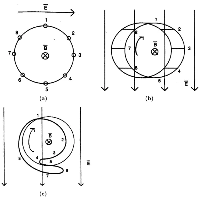
As we have learned, the gyrotron interaction (or CRM interaction) occurs in the cavity region of the gyrotron. First we will discuss the fundamental mode interaction, ignoring variations in the electric field across the Larmor radius. Fig. 2-3(a) shows a cross-section of the electron beam at the beginning of the interaction region. As the beam progresses into the cavity, the transverse electric field will exert a FRF

-qERF force that will cause some electrons to accelerate and others to decelerate, depending on the relative phase of the electric field. In Fig. 2-3(b), electrons 2, 3, and 4 are decelerated, while electrons 6, 7, and 8 are accelerated, and electrons 1 and 5 are undisturbed. This perturbation results in a change of energy. If an electron gains energy, the relativistic factor y increases, which decreases the electron cyclotron frequency w, and increases the Larmor radius rL. On the other hand, if an electron loses energy, -y decreases which causes w, to increase and rL to decrease. After a few cycles, the electrons that gained energy lag in phase and the electrons that lost energy advance in phase. Soon, the electrons have formed a bunch (Fig. 2-3(c)). If the frequency of the electric field is exactly equal to the electron cyclotron frequency, the bunch will not gain or lose energy. In order to extract power from the beam, the bunch must be formed at a field maximum. If the axial magnetic field is tuned such that the RF frequency w is slightly greater than the cyclotron frequency w,, then the bunches will orbit in phase and transfer their rotational energy to the TE field mode, increasing the field strength and encouraging more bunching. This domino effect results in a rapid amplification of the dominant mode.

1 8 2 7 ₃ 6 4 5 (a) I

C

8>4 3 5 7 I

-I

(C 5 (b) (c)

Figure 2-3: Gyrotron phase bunching: (a) initial condition, where the electrons are uniformly distributed on a beamlet (b) new positions of the electrons immediately after the change in energy (c) formation of the electron bunch [4]

2

3

Harmonic CRM interaction

The fundamental interaction is not the only possible interaction that can occur to transfer energy from the beam to RF field. If the electric field varies across the Larmor radius, it is possible to have a harmonic interaction. A quadrapole electric field is required for a second harmonic interaction, as shown in Fig. 2-4, where the electrons gain energy in the 1 > 0 region and lose energy in the - < 0 region. A

hexapole field would be required for a third harmonic interaction, etc. Two bunches of electrons may be formed during a second harmonic interaction. Up to n bunches may be formed when operating at the nth harmonic. The resonance condition is now

w =i nw for operation at the nth harmonic.

In order to excite a second harmonic interaction, a stronger second harmonic than fundamental electric field must be experienced by the beam. There are two meth-ods by which this can be accomplished. The first method relies on the beam being positioned where the coupling to the second harmonic field is stronger. Otherwise, a stronger second harmonic electric field is necessary, if the coupling to the second harmonic and fundamental modes is comparable [4].

Weibel instability

The gain mechanism for gyrotrons, the CRM interaction described in this section, is caused by the azimuthal bunching of electrons. There is also a mechanism which causes axial bunching of electrons, a Lorentz force interaction between the electrons and the RF magnetic field, known as the Weibel instability [26]. The Weibel insta-bility and the CRM interaction compete with each other, but one usually dominates [27]. In a fast-wave device, the CRM interaction (also know as the gyrotron interac-tion) is the dominant one. Since gyrotrons operate near cutoff, k1

>>

k11. And k1vjj is

small, so the fast-wave condition of the phase velocity,

v = > C (2.50)

holds true.

)4'

I I

I

Figure 2-4: Quadrapole electric field for a second harmonic interaction [4]

2.1.3

Non-linear theory

To develop a non-linear theory for a gyrotron oscillator, we begin with the equations of motion for an electron moving in an electromagnetic field,

=t -e -E (2.51)

dt

dt c (2.52)

where 9 = ymec2 _{is the electron energy, -y = (1 - v}2_/c 2_)- 1_/2_{, and Ip1 = 'ymec}2 _{is the}

electron momentum.

Normalized parameters

Assuming that the electric field is a TE cavity mode, we can write the transverse efficiency r I, the fraction of transverse power that has been transferred to the RF

field, in terms of four normalized parameters [5], F = Bfo n!2n-1) Jmjn(kireo) (2.53) B o Ln2-= L _(2.54) A = 1 - (2.55) ±0 V±O (2.56) C

where F is the normalized field amplitude, p is the normalized cavity interaction

length, A is the detuning between the wave frequency and the electron cyclotron

fre-quency, w, = eB/-ym (magnetic field parameter), and O3 _o is the normalized transverse

velocity at the entrance to the cavity.

In addition, a normalized energy variable,

U = 2 1 - -(2.57)

and a normalized axial position variable,

r= 0r ± (2.58)

have been defined.

If the electron beam is weakly relativistic and nO31 < 1, then ql is reduced to being a function of only F, p, and A. The beam current can be related to the field amplitude F by an energy balance equation. The total cavity

Q,

QT, can be written

in terms of the total stored energy U and the power dissipated P,

T = WU (2.59)

where the dissipated power P is given by

P = IAV, (2.60)

IA is the beam current, and V is the cathode voltage. Evaluating the stored energy with a Gaussian axial field profile, the energy balance equation is derived as

F2 _{= r1I, (2.61)}

where the normalized current parameter I is defined by

I = 0.238 x i0- QTIA) 2(-3) X xn (A)

( )

2 Jm±n(kireo) (2.62) \ 7=

0 .238

0 L 2 / (v m2 - m 2_)J

2 (Vm p)

Efficiency

Fig. 2-5 shows contour curves of qL, at second harmonic operation, as a function of F and [, optimized with respect to the magnetic field parameter A, with the optimum value at Apt. The curves are shown for second harmonic operation, since that is the design being presented in this work. For the second harmonic interaction, peak perpendicular efficiencies of over 70% are theoretically possible.

The total efficiency also accounts for voltage depression and parallel energy. 7k, is the fraction of beam power in the perpendicular direction and T/Q is the reduction due to ohmic losses.

7T =7el X 7Q X 71 (2.63) #0 x QOHMQOH x 771 (2.64) 2(1- 7 1_{) QD + QOHM} Pou P o u ( 2 .6 5 ) IV

where I is the beam current and V is the beam voltage,

QT =QOHMQD QOHM + QD is the total

Q,

TM ( 22 QOHM = -o 1 2 (2.67) 6 _m~p

0.17--.75 ~~03 IIM I ApN 0.01

Av

2

0

10

20

₃₀

₄₀

Figure 2-5: Transverse efficiency contour r/, (solid line) as a function of the normalized field amplitude F and normalized effective interaction length p for optimum detuning

A (dashed line) and second harmonic n = 2 [5]

is the ohmic

Q,

6 is the skin depth, QD is the diffractive

Q,

QD = 47 (L/A)2 (2.68)

1 - JR1,21

and R₁,2 is the wave reflection coefficient of the input and output cross-sections of a resonator.

Starting current

The starting current Ist can be numerically calculated as a function of magnetic field for a given mode. Two codes that are used to calculate the starting current, LINEAR

[28] and CAVRF [29] will be discussed.

The diffractive

Q

from Eq. 2.68 and the effective interaction length from Eq. 2.54 need to be calculated numerically. These quantities can be calculated by the code CAVRF developed by A. Fliflet at the Naval Research Laboratory, which solves for the eigenmodes of a cold gyrotron cavity (in the absence of an electron beam). The effective interaction length is defined as the axial distance between which the RF field amplitude is greater than 1/e times the maximum RF field amplitude.

Now using the total

Q

and the effective interaction length determined by CAVRF, we can calculate the starting current with the code LINEAR developed by K. Kreis-cher at MIT. LINEAR calculates the starting current for a Gaussian or sinusoidal RF field profile in a cylindrical open resonator, assuming that adiabatic theory is valid in the gun region, and the electron beam is monoenergetic annular azimuthally symmet-ric with no radial thickness or velocity spread. To calculate the linear characteristics, several device parameters must be user-specified: beam and anode voltages, cavity and cathode magnetic fields, mode and harmonic numbers, cavity radius, effective cavity interaction length, cathode/anode distance, ohmic

Q,

diffractive

Q,

and the cathode radius. Using this data, the starting current is calculated as a function of the magnetic field.

2.1.4

Second harmonic challenges

The excitation of the second harmonic can be quite challenging. At lower frequencies, harmonic modes are observed when there is a gap in the fundamental spectrum, [30] however the fundamental spectrum becomes dense at frequencies above 300 GHz [4].

Foremost, the starting current of the second harmonic is at least 1.6 times higher than that of the fundamental modes, resulting in the suppression of harmonic modes in favor of the fundamental. In the linear regime, the normalized starting current becomes

4 ed~

Ist = 2 (2.69)

7A p -, n

where x = pA/4. Using the normalized current parameter Eq. 2.62, and assuming the coupling coefficient Cmp from Eq. 2.49 is proportional to the square of the wavelength and the linear normalized starting current Ist from Eq. 2.69 is proportional to i/Pu3, we find an expression for the ratio between starting currents for the nth harmonic and the fundamental [31],

T 1 2 ( 1 - n )

( . 0

In, QTli/3'Y _(2.70)

I, Qrn

This expression tells us that we can lower the starting current by either raising the cavity

Q

or the velocity ratio a (by raising the normalized perpendicular velocity i31o). Since in this experiment an existing gun design is being used, increasing

#J-o

can only be achieved to a certain degree. However it is possible to design for a higher cavity

Q.

Secondly, in order to reduce ohmic losses, the highly overmoded cavities required make mode competition more severe; the mode density increases as the cavity size becomes larger.

Thirdly, a thick beam can couple simultaneously to several different modes. When operating at a second harmonic mode, the beam can effectively couple to the design mode as well as one or two fundamental modes and several other harmonic modes.

In order to excite a second harmonic mode, we can clearly see that the fundamental modes need to be suppressed. In this thesis, this has been attempted through clever

design of lowering the starting current for the desired second harmonic mode and selecting a mode that is relatively isolated from the fundamentals.

2.2

Nuclear magnetic resonance

The principal motivation for this gyrotron design is in high-field DNP NMR studies. In order to better understand this application, we present a brief overview of the theoretical foundations of of this experiment.

Nuclear magnetic resonance is a powerful and routine spectroscopic technique for the study of structure and dynamics in condensed phases and, in particular, of biological macromolecules. Its prinicipal limitation is low sensitivity; the small nuclear Zeeman energy splittings result in correspondingly small nuclear spin polarization at thermal equilibrium [23]: Nm - I -Emi Nm= exp(-Em)/exp (-) (2.71) N kBT e=- kBT (mh-Bo I m(mhBo( = exp

/

_ exp BT (2.72) mh-yBo I -,gBo 1+ / 1 (1 + h (2.73) kBT M=-I kBT mh-yBo (I + /o /(21+1) (2.74)

where Nm is the number of nuclei in the mth state (-1 or 1 for a spin-! nucleus), N is the total number of spins, T is the absolute temperature, kB is the Boltzmann constant, Em = -mh-yBo is the nuclear Zeeman energy, h is Planck's constant divided

by 27r, BO is the static magnetic field, I is the nuclear spin angular momentum, and we have taken the high temperature limit in Eq. 2.74. For example, protons at room temperature exhibit a spin polarization of less than 0.01% in a field of 5 T [15]. Though both solution and solid state NMR suffer from this poor sensitivity, relaxation processes in the solid state further compromise the time-averaged sensitivity of these experiments by two or three orders of magnitude. The low sensitivity of SSNMR

complicates the study of biological systems, where sample amounts are limited and spectra are complex.

2.2.1

Dynamic nuclear polarization

Dynamic Nuclear Polarization (DNP) is a magnetic resonance technique used to en-hance the polarization of nuclei through interactions with the electron spin popu-lation. It occurs through a variety of mechanisms, all involving irradiation of the electron spins at or near their Larmor frequency. The effect was first observed in

1956 by Carver and Slichter [32] and later in 1958 by Abragam and Proctor [33]. His-torically, it has been used to enhance the polarization of targets in nuclear scattering experiments, in sensitivity enhancement in the NMR of amorphous solids, and, re-cently, for sensitivity enhancement in high resolution NMR spectroscopy. There are three principal polarization transfer mechanisms: the solid effect, thermal mixing, and the Overhauser effect.

Solid effect

The solid effect, also known as the solid state effect, occurs in solids with fixed param-agnetic centers where the time-averaged value of the anisotropic hyperfine interaction is not zero [34]. In these systems, the spatial part of the hyperfine interaction can be described by a stationary Hamiltonian; as a result, the electron-nuclear spin system is no longer described by pure tensor product states alone, and we must admit a small admixture of states in the electron-nuclear wave function. The consequence of this admission is that so-called "forbidden transitions" involving simultaneous nuclear and electron spin flips can occur with small probability if the system is irradiated near

w = We ± w,. These transitions give rise to polarization enhancements of the nuclear spin population, where the enhancement is given by [35]

ESE B T1n (2.75)

n bW (BO 40

where the electron and nuclear gyromagnetic ratios Ye and N respectively are defined by the ratio of the frequency

f

_{to the static magnetic field Bo,}

7Yp,e fpe (2.76)

Bo

= 42.6 MHz/T for protons (2.77)

= 28.0 GHz/T for electrons (2.78)

a contains physical constants, Ne is the density of unpaired electrons, J is the EPR linewidth, b is the nuclear spin diffusion barrier, B1 is the microwave field strength,

and Tin is the nuclear spin-lattice relaxation time.

Thermal mixing

The most useful mechanism of polarization enhancement in these high-field DNP studies has been thermal mixing. Thermal mixing occurs in systems with fixed para-magnetic centers at high concentration, such that the ESR line is homogeneously broadened. Under these conditions, a thermodynamic and separable treatment of electron-electron and electron-nuclear interactions is possible. In this treatment, three thermal reservoirs corresponding to the Zeeman system, the spin-spin inter-action system, and the lattice are at thermal equilibrium [36]. Irradiation near the electron Larmor frequency can produce nuclear polarization enhancements through a variety of mechanisms, with the enhancement approximately given by [35]

eNN2 B 2

ETM =a - eB- TnTe (2.79)

,62 _BO)

where a' contains physical constants and Te is the electronic nuclear relaxation time. So in principle, signal enhancements on the order of -ye/-Yn can be obtained. This corresponds to a factor of 657 for 1H nuclei and 2615 for 13_{C nuclei.}

Though these mechanisms all play roles in enhancing the sensitivity, studies show that thermal mixing is the predominant effect. Using a 140 GHz gyrotron, we have

previously demonstrated that signal enhancements of several orders of magnitude (100 - _{400) are achievable at a magnetic field of 5 T [15, 16, 17, 18, 19, 37]. However,} to obtain higher resolution spectra, it is desirable to perform DNP at higher field strengths (9 - 18 T), where NMR is commonly employed today.

There are several problems encountered when performing DNP at high fields. First, the enhancement decreases as 1/B2 with increasing static field strength for the solid effect and as 1/BO for thermal mixing as indicated by Eqs. 2.75 and 2.79. Second, relaxation mechanisms responsible for the DNP effect are fundamentally dif-ferent at higher fields. These problems at high field can be overcome, and significant signal enhancements obtained, by using high radical concentrations and high mi-crowave driving powers. Furthermore, the enhancements scale with the square of the microwave driving field and only inversely with the applied magnetic field. Therefore, large signal enhancements can be achieved, even at high fields (9 - 18 T) if sufficient microwave power (1 - 10 W) is available to drive the polarization transfer.

Chapter 3

460 GHz Gyrotron Design

Other millimeter wave sources, such as the EIO (extended interaction oscillator) or BWO (backward wave oscillator) rely on fragile slow-wave structures to generate microwave radiation, and thus at the high power levels required for DNP experiments have limited operating lifetimes. Consequently gyrotrons are the only feasible choice for generating such high microwave powers at high frequencies (100 - 1000 GHz). This has been the motivation for the 250 GHz gyrotron [21] recently constructed at the Plasma Science and Fusion Center which allows DNP-NMR experiments to be performed in a routine manner and the presented design of a 460 GHz gyrotron.

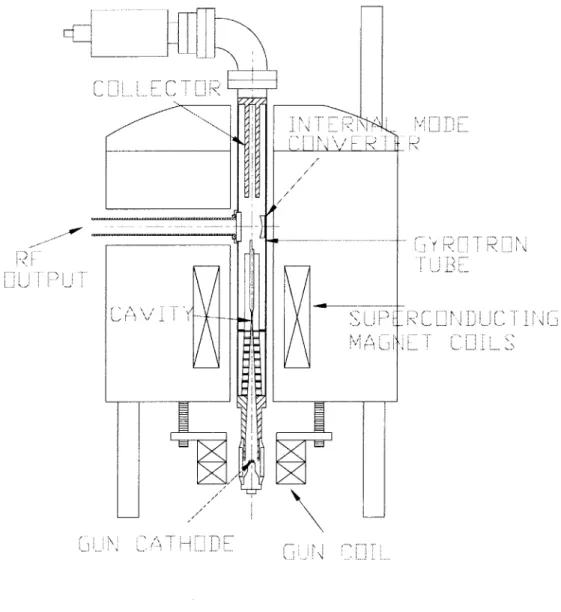
A schematic of the 460 GHz gyrotron is depicted in Fig. 3-1. Starting from the bottom of the picture, the electron beam is generated by the electron gun. The mag-netic field of the gun region is adjusted using the gun coil. The beam is compressed by an axial magnetic field provided by the superconducting magnet. The cavity, located in the center of the magnetic field, is where the the electron beam energy is extracted. The electron beam is collected at the collector. The RF beam is launched into free space in the mode converter where it becomes a Gaussian beam and is reflected out a side vacuum window.

]

N', / / / / / / Ef _/

H.*

Figure 3-1: Schematic of the 460 GHz gyrotron for DNP

Table 3.1: Comparison of important 250 and 460 GHz gyrotron design parameters

3.1

250 GHz gyrotron

Our design is based upon the 250 GHz gyrotron used for DNP studies, designed by K. Kreischer [21]. A summary of the design parameters of the tube can be found in [20] and Table 3.1. The gyrotron operates in the fundamental TE 31 mode at a frequency of 250 GHz and magnetic field of about 9 T. An output power of 25 W at continuous wave operation can be generated.

The present design incorporates the same electron gun as the previous design, limiting certain factors, such as the beam velocity ratio a. The frequency chosen matches NMR magnetic field 16.4 T.

3.2

Cavity design

The gyrotron cavity is where the electron beam transfers energy to the transverse electric field mode. With a good design, the microwave radiation can be extracted at high efficiency levels. The design of the optimal cavity has been determined through the use of several codes. There are several constraining parameters for the design of the cavity that are presented, emanating from NMR and second harmonic consider-ations. The final cavity design including the RF field profile is pictured in Fig. 3.2

460 GHz 250 GHz

Mode _{TE061 TE031}

Harmonic number 2 1 Frequency (GHz) 460 250 Magnetic Field (T) 8.39 9.06 Diffractive

Q

37,770 4,950 Total

Q

13,650 3,400 Cavity Radius (mm) 2.04 1.94 Cavity Length (mm) 25 18

Cavity Beam Radius (mm) 1.03 1.02

Beam Voltage (kV) 12 12

Beam Current (mA) 97 40

Table 3.2: Gyrotron cavity design parameters Mode TE06 1 Frequency (GHz) 460 Magnetic Field (T) 8.39 Diffractive

Q

37,770 Total

Q

12,950 Cavity Radius (mm) 2.04 Cavity Length (mm) 25

Table 3.3: Beam extraction parameters

using the design parameters from Table 3.2 and 3.3.

3.2.1

NMR considerations

A 17 T, high-resolution, NMR magnet corresponding to a proton Larmor frequency of 700 MHz (16.4 T) has been acquired for use with a DNP NMR spectrometer. The DNP NMR experiment requires a matching of proton and electron fields. The ratio of the proton frequency to the gyrotron frequency is thus equal to the ratio of their respective gyromagnetic ratios:

fe = f, '7P 28.0 x 10 9 700 x 106 _{42.6 x 106} = 460 GHz (3.1) (3.2) (3.3)

The corresponding frequency needed to be generated by the gyrotron is 460 GHz. Previous dynamic nuclear polarization experiments driven by 140 and 250 GHz

46

Cavity Beam Radius (mm) 1.03

Beam Voltage (kV) 12

Beam Current (mA) 97

Beam Velocity Ratio a 2

Power (W) 50

req=459.953 GHz

=37715.61

A=1.9

ea

ohm=

.05

ea -.

000%

.07

u

38.22

IZI

-gyrotrons indicate that a CW power capability of 10-100 W is sufficient to extend DNP into higher fields [15, 16, 17, 20]. A design power of 50 W has been chosen to meet this need.

3.2.2

Second harmonic

In section 2.1.4, we discussed the challenges of realizing the second harmonic, such as a higher starting current and coupling of the beam of finite thickness to multiple modes. These theoretical issues may evolve into design issues that need to be addressed.

Operating mode

In order to operate at a higher frequency, we are selecting a second harmonic mode of operation. Fundamental modes have much lower starting currents, thus the mode we select must be sufficiently free from such fundamental modes and also other second harmonic modes, as seen in Sec. 2.1.3.

We must ensure that there is a gap in the frequency spectrum in which our mode is situated. Recall from Eq. 2.47 that the frequency f of a TEmp mode can be approximated by

f = Cump (3.4)

and from the resonance condition Eq. 2.48 that vmpl ~ jVmp2, where 1 denotes the fundamental and 2 the second harmonic modes. We see from Eq. 3.4 that gaps in the frequency spectrum are a direct result of spacing of the TE mode indices, vmp. To avoid interference from fundamental modes, we must choose a second harmonic mode where half of the value of its index,

jVmp2,

is in a sizable gap between consecutive fundamental mode indices vmp1. After examining the mode spectrum in Fig. 3-3 we chose TE0 6, whose mode index is located between the fundamental modes TE8 1 and

TE₂₃.

The gap in mode indices where our second harmonic mode is located should trans-late into a region in the magnetic field where our mode can be excited without com-petition from the fundamental. Fig. 3-4 shows a plot of the starting currents of modes