Hounsfield unit recovery in clinical cone beam CT images of the thorax acquired for image guided radiation therapy

Publisher’s version / Version de l'éditeur:

Physics in Medicine and Biology, 61, pp. 5781-5802, 2016-07-13

READ THESE TERMS AND CONDITIONS CAREFULLY BEFORE USING THIS WEBSITE. https://nrc-publications.canada.ca/eng/copyright

Vous avez des questions? Nous pouvons vous aider. Pour communiquer directement avec un auteur, consultez la Questions? Contact the NRC Publications Archive team at

PublicationsArchive-ArchivesPublications@nrc-cnrc.gc.ca. If you wish to email the authors directly, please see the first page of the publication for their contact information.

Archives des publications du CNRC

This publication could be one of several versions: author’s original, accepted manuscript or the publisher’s version. / La version de cette publication peut être l’une des suivantes : la version prépublication de l’auteur, la version acceptée du manuscrit ou la version de l’éditeur.

For the publisher’s version, please access the DOI link below./ Pour consulter la version de l’éditeur, utilisez le lien DOI ci-dessous.

https://doi.org/10.1088/0031-9155/61/15/5781

Access and use of this website and the material on it are subject to the Terms and Conditions set forth at

Hounsfield unit recovery in clinical cone beam CT images of the thorax

acquired for image guided radiation therapy

Thing, Rune Slot; Bernchou, Uffe; Mainegra-Hing, Ernesto; Hansen, Olfred;

Brink, Carsten

https://publications-cnrc.canada.ca/fra/droits

L’accès à ce site Web et l’utilisation de son contenu sont assujettis aux conditions présentées dans le site LISEZ CES CONDITIONS ATTENTIVEMENT AVANT D’UTILISER CE SITE WEB.

NRC Publications Record / Notice d'Archives des publications de CNRC:

Hounsield unit recovery in clinical cone

beam CT images of the thorax acquired

for image guided radiation therapy

Rune Slot Thing1,2_{, Uffe Bernchou}1,2_{, Ernesto Mainegra-Hing}3_, Olfred Hansen1,4 _{and Carsten Brink}1,2

1 _{Institute of Clinical Research, University of Southern Denmark, Odense, Denmark} 2 _{Laboratory of Radiation Physics, Odense University Hospital, Odense, Denmark} 3 _{Ionizing Radiation Standards, National Research Council of Canada, Ottawa K1A} 0R6, Canada

4 _{Department of Oncology, Odense University Hospital, Odense, Denmark}

E-mail: rune.slot.thing@rsyd.dk, uffe.bernchou@rsyd.dk,

ernesto.mainegra-hing@nrc-cnrc.gc.ca, olfred.hansen@rsyd.dk and carsten.brink@rsyd.dk

Received 23 December 2015, revised 27 April 2016 Accepted for publication 15 June 2016

Published 13 July 2016

Abstract

A comprehensive artefact correction method for clinical cone beam CT (CBCT) images acquired for image guided radiation therapy (IGRT) on a commercial system is presented. The method is demonstrated to reduce artefacts and recover CT-like Hounsield units (HU) in reconstructed CBCT images of ive lung cancer patients.

Projection image based artefact corrections of image lag, detector scatter, body scatter and beam hardening are described and applied to CBCT images of ive lung cancer patients. Image quality is evaluated through visual appearance of the reconstructed images, HU-correspondence with the planning CT images, and total volume HU error.

Artefacts are reduced and CT-like HUs are recovered in the artefact corrected CBCT images. Visual inspection conirms that artefacts are indeed suppressed by the proposed method, and the HU root mean square difference between reconstructed CBCTs and the reference CT images are reduced by 31% when using the artefact corrections compared to the standard clinical CBCT reconstruction.

A versatile artefact correction method for clinical CBCT images acquired for IGRT has been developed. HU values are recovered in the corrected CBCT

Original content from this work may be used under the terms of the Creative Commons Attribution 3.0 licence. Any further distribution of this work must maintain attribution to the author(s) and the title of the work, journal citation and DOI.

images. The proposed method relies on post processing of clinical projection images, and does not require patient speciic optimisation. It is thus a powerful tool for image quality improvement of large numbers of CBCT images.

Keywords: cone beam CT, image guided radiotherapy, image quality, Monte Carlo

(Some igures may appear in colour only in the online journal)

1. Introduction

As cone beam CT (CBCT) imaging for image guided radiation therapy (IGRT) is becoming standard practice in many centres, the potential use of CBCT imaging as a basis for person-alised radiotherapy is proposed in numerous ways. Dose calculation and accumulation has been proposed by many studies, with online adaptive replanning as the most challenging and desirable application (Yang et al 2007, Rong et al 2010, Fotina et al 2012, Elstrøm et al 2014, Vestergaard et al 2014).

For lung cancer patients in particular, anatomical changes occur frequently, requiring treat-ment plan adaptation to deliver the intended radiation dose to the target while sparing the organs at risk (Møller et al 2014). Such adaptations are labour intensive, and it is desirable to be able to use the CBCT images acquired for IGRT to either perform the plan adaptation and replanning, or determine for which patients a new CT scan and replanning procedure is required dosimetrically. Another more recent application of CBCT images of the thoracic region is the extraction of biomarkers to predict tumour control or toxicity measures during treatment of lung cancer, with a view to differentiating the patient population based on their radiosensitivity (Bertelsen et al 2011, Brink et al 2014, Jabbour et al 2015, Bernchou et al

2015). Such differentiation has the potential of providing better tumour control rates for those patients who can tolerate higher dose levels, while providing a better quality of life for those patients who are prone to severe toxic sideeffects such as pneumonitis and pulmonary ibrosis.

The main limiting factor for all of the above mentioned extended uses of CBCT images is the image quality. CBCT image quality has been studied since the irst gantry mounted CBCT scanner was realised (Jaffray et al 2002), with ive different factors known as the main causes for the limited image quality, namely image lag (Siewerdsen and Jaffray 1999), detector scat-ter (Poludniowski et  al 2011), body scatter (Siewerdsen and Jaffray 2001), beam hardening (Herman 1979), and a potential truncated ield of view (Ohnesorge et al 2000). Each factor has been studied extensively using different phantoms, but to our knowledge no study has yet inves-tigated the potential increased image quality when all artefact sources are considered together in relation to clinical CBCT imaging of patients. This study investigates how clinical CBCT images of the chest can be improved by correcting for all ive artefact sources. Post-processing of raw image data from the Elekta XVI CBCT system is performed, and we demonstrate that proper Hounsield Units (HUs) can be recovered from the existing projection images.

2. Materials and methods

All CBCT scans were acquired on the Elekta XVI R4.5 system, either mounted on an Elekta Versa HD or an Elekta Synergy accelerator (Elekta Ltd, Crawley, UK). The XVI R4.5 CBCT system is based on a Dunlee type DA1094/DU694 x-ray tube (Dunlee, IL, USA) and a PerkinElmer XRD 1640 lat panel imager (PerkinElmer Inc, MA, USA).

Five lung cancer patients were chosen from our clinical database, selected to have had a CBCT scan and a re-simulation CT (rCT) scan performed on the same day to facilitate a comparison between CBCT and CT image quality. CBCT scans were acquired using the small ield of view without bowtie iltration, allowing a cylindrical volume of length 276.6 mm and diameter 270 mm to be reconstructed. For each scan, approximately 750 frames were acquired over an arc of 220°, using our clinical protocol for fast 4D CBCT imaging. Each frame was exposed to 0.32 mAs, and acquired at a ixed frame rate of 5.5 Hz. The CBCT images were acquired as 4D scans in the clinic, but were reconstructed in 3D in the present work. All patients were scanned isocentrically, with only small (⩽1 cm) couch shifts applied prior to treatment. In the following sections, all the applied image corrections will be described briely to provide the full overview of artefact corrections.

2.1. CBCT reconstructions

A total of four reconstructions were made from each CBCT scan. A schematic drawing of the image processing associated with each of the four reconstructions is shown in igure 1.

2.1.1. XVI. For reference, a CBCT reconstruction was made using our standard clinical preset for 3D reconstruction in the XVI software. This uses a simple scatter correction, where the scatter in each projection image is estimated as a fraction of the mean signal in all pixels with a reading of less than ₃₂×₁₀3_{. In our clinic, the scatter subtraction was found to be optimal}

at 20% of the mean signal in each projection. If the scatter correction results in pixel values less than 20, a constant is added to the entire projection image to ensure the minimum value is 20. The XVI projection images are stored as 16 bit integer images, thus containing 216 gray levels. Following the scatter correction, XVI uses a standard FDK-type iltered backprojection algorithm (Feldkamp et al 1984) to reconstruct the CBCT images. No information about the use of truncation correction in the XVI system was available. This clinical reconstruction will be denoted XVI.

2.1.2. RTK(XVI). To investigate the effects of changing the reconstruction algorithm from the XVI native to the FDK-type algorithm provided with the reconstruction toolkit (RTK) (Rit et al 2014), a reconstruction was made using a similar scatter correction method as that in the XVI software prior to reconstruction. Furthermore, a 2D median ilter with a Figure 1. Overview of the image processing and reconstruction for each of the four different CBCT reconstructions. The XVI method is the clinical reference method.

RTK(XVI) resembles the XVI method, but uses RTK to perform the image reconstruction. RTK(BS) uses Monte Carlo based scatter correction and RTK reconstruction, while RTK(All) includes correction for image lag, detector scatter, MC based body scatter

×

5 5 pixel kernel was applied to the projection images prior to reconstruction, similar to what is used inherently by XVI. The use of RTK allows for truncation correction based on the work of Ohnesorge et al (2000), which was used to approximate the truncated anatomy as going to zero over a distance of 20% of the projection image size. Additionally, a Hann window set to a cut-off frequency of 0.8 was used to reduce high frequency noise in the reconstructed images. This reconstruction is referred to as RTK(XVI), and was included in the comparison to emphasise the difference in image quality resulting from changing the reconstruction algorithm only, while keeping image corrections similar to the clinical implementation in XVI.

2.1.3. RTK(BS). With the main reason for poor CBCT image quality being body scatter from the patient, a reconstruction was made using an MC based scatter correction method developed from our previously published model (Thing et al 2013). The EGSnrc (Kawrakow 2000, Kawrakow et  al 2011) user code egs_cbct (Mainegra-Hing and Kawrakow 2008, 2010) was used to provide fast MC simulations of patient speciic scatter distributions, taking advantage of the variance reduction techniques (VRTs) implemented in egs_cbct (Thing and Mainegra-Hing 2014). To provide accurate scatter estimates, the full x-ray source was simulated using a compiled BEAM source in egs_cbct (Rogers et al 2011). Speciications of the x-ray tube and collimation were found in manuals and data sheets of the Dunlee tube and the XVI system, and details of the source simulation is provided in appendix A. Photon interaction cross sections from the XCOM compilation (Hubbell and Seltzer 2004) were used, with Rayleigh scattering included in the simulations. Photon low energy cut-off was set to 1 keV in the entire simulation geometry, and to avoid spending time simulating electrons which do not reach the detector, the electron low energy cut off was set to 1 MeV after the primary collimation and iltration of x-rays from the BEAM source.

In addition to the scatter calculations, primary photons were simulated to allow an appro-priate normalisation between simulated and clinical projection images. The primary simula-tion was performed using a spatially uniform source with an energy distribusimula-tion obtained from the full MC simulation of the XVI source. To facilitate fast calculations, a ray tracing mode was implemented in egs_cbct and used for the primary calculations. All simulated projec-tion images were normalised to open ield simulaprojec-tions.

The energy response of the XVI lat panel detector was adopted from Roberts et al (2008). In the present work, the full detector resolution of 512×512 quadratic pixels with a side

length of 0.8 mm was used, and projection images were simulated at an angular interval of 2.5°.

Patient speciic primary and scatter simulations were allowed through the creation of a simulation phantom based on the planning CT image for each patient. Four different tissues were assigned based on the HU in each voxel of the planning CT, namely air, lung tissue, soft tissue, and bone. Within each tissue, the density varies according to the exact HU found in each CT voxel. With the simulations based on the planning CT, it is possible to perform all MC calculations prior to CBCT acquisition.

Based on the assumption that the simulated total signal equals the measured clinical projec-tion images when normalised to the appropriate open ield signal (ISim/I ₌I /I

0

Sim Clin 0 Clin

), the scatter subtraction is obtained through a simple scaling of the simulated scatter signal:

= − ⋅

I I K I

I .

MC

Clin Clin scatterSim 0 Sim

Here, IClin _{denotes the measured clinical projection images, and I} scatter Sim

the simulated scatter signal. K is equivalent to the average clinical open ield signal ⟨I0Clin⟩; a quantity which is not

measured or stored in the XVI system. Therefore, it was estimated retrospectively in the fol-lowing way: For each set of projection images, a smoothed histogram was calculated for both the clinical and simulated projections. The histograms were created with 100 equidistant bins spanning the full range of numbers in the projection image sets. In these two histograms, two distinct peaks were visible, corresponding to signal attenuated by soft tissue or air. These two peaks were used to perform a two-point calibration of K through

    = − − K H H H H air Clin soft tissue Clin air Sim soft tissue Sim (2)

where H denotes the mean value in the most frequent histogram bins corresponding to air and soft tissue. When determining the scaling factor K through the proposed histogram analysis, the requirement of accurate patient positioning (potentially obtained by rigid or deformable image registration) is relaxed due to the low frequency variation found in the scatter signal (Thing et al 2013). Therefore, the isocentric patient setup prior to CBCT acquisition was suf-iciently accurate for the MC based body scatter correction to be applied.

While equation (1) is conceptually very simple, it has the potential of leading to negative values of I_MCClin behind highly attenuating anatomy or in the case of severe image noise. To avoid these undesired negative numbers, a smooth cut-off function adapted from Xu et  al (2015) was used in the present study. A γ parameter is deined through the scatter to total ratio:

/ γ = I ≈ ⋅ I K I I I . scatter total

scatterSim 0Sim Clin

(3)

Here, the approximation is used to emphasize measurement noise and non-ideal behaviour in the imaging chain, as well as approximations made in the MC simulation. Based on this deinition of γ and a cut-off ratio of β_{= 0.7} (determined empirically), the scatter corrected signal IMCClin was calculated as:

( )     ⩽ ⩽ ( )     ⎧ ⎨ ⎪ ⎩ ⎪ ⎡ ⎣ ⎢ ⎛ ⎝ ⎜ ⎞ ⎠ ⎟ ⎤ ⎦ ⎥ γ γ β β γ β β γ β = ⋅ − ⋅ − ⋅ − − − > I I I 1 for 0 1 exp 1 for . MC Clin Clin Clin (4)

This formalism reduces to equation  (1) for γ⩽β (full scatter correction), while for larger scatter to total ratios, the scatter subtraction is gradually decreased such that the remaining signal I_MCClin tends towards zero. Equation (4) is derived from the constraints that I_MCClin and its irst derivative in γ must be continuous, and that IClinMC→0 as γ→∞.

Before reconstruction, the scatter corrected projection images were rescaled by the open ield signal estimated through (2):

= ⋅ I I K 2 . rescaled Clin ClinMC 16 (5)

This rescaling is applied since RTK expects the open ield signal in projection images to have a digital value of 216_{, and a completely blocked signal to have a digital value of 0. The}

rescaled images were median iltered and reconstructed in RTK as described in the previous RTK(XVI) method. This method of body scatter correction and RTK reconstruction is referred to as RTK(BS).

2.1.4. RTK(All). The most sophisticated artefact correction method included ive steps prior to reconstruction, each of which is described in the following. The order in which to apply the corrections was determined to irst correct for the physical effect which occurs last, and then work backwards from the detector related artefact sources to the patient related artefact sources. Thus, the corrections in applied order were image lag, detector scatter, body scatter, and beam hardening, before projection scaling was performed prior to CBCT reconstruc-tion with truncareconstruc-tion correcreconstruc-tion applied. This comprehensive correcreconstruc-tion and reconstrucreconstruc-tion is denoted RTK(All).

Image lag. A linear time invariant image lag correction method was developed based on the works by Hsieh, Starman and Mail (Hsieh et al 2000, Mail et al 2008, Starman et al 2011,

2012). Such a model assumes that some signal will be trapped in the detector and not be read out in the correct frame. This leads to a situation where each frame from the detector contains signal from the previously exposed frames, as well as signal from the current exposure. Fur-thermore, some signal from the current exposure will be stored and read out in the following frames.

In the present model, the time function of the measured signal Imeas _{from a very short}

expo-sure Iexp _{(a delta function) is described as a sum of exponentials:}

( ) ⎛ ⎝ ⎜ ⎞ ⎠ ⎟

∑

Here, ai is the amplitude of each exponential term, ti the decay time of each term, and n is the

number of exponentials required to describe the decaying signal. ai is bound by the constraint

that ∑ai=1, and it is noted that the irst exponential in the sum has a large amplitude and

short decay time, corresponding to the fact that most of the signal from a delta pulse is read out in the irst frame.

For continuous exposures, a set of signal storage variables qi is introduced, each of which

is updated frame by frame. The lag correction model of the time dependent detector readout corrects for increases in signal from the previous frames, as well as a lack of signal from the present frame which is stored for future frames. Given a set of measured projections {IClin( )}k _,

where k denotes the frame number starting at k = 1, the lag corrected signal {ILagCorrClin ( )}k is

calculated as ( ) ( ) ( ) ( ( / )) ( / ) = − ∑ ⋅ − −∆ − ∑ −∆ = = I k I k q k k t a k t 1 exp 1 exp i n i i i n i i LagCorr Clin Clin 1 1 (7)

where ∆k is the time between frames. All parameters but ∆k were determined experimentally. In the present study, the time was measured in units of the ixed time between frames on the XVI R4.5 system (181 ms), and hence ∆ =_{k 1. qi is deined recursively with qi(k = 1) = 0 and}

( + )=[ ( )⋅ + ( )]⋅ (−∆ / )

q k_i 1 ILagCorrClin k ai q ki exp k ti .

(8) To determine ai and ti, a number of calibration measurements were performed using the

falling step response method. To obtain the calibration measurements, the XVI unit was oper-ated in service mode where it is possible to have continuous readout of the detector while the x-ray source can be turned on and off independently. Measurements were acquired with the x-ray source turned on before the frame readout was enabled. After readout of approximately 200 exposed frames, the x-ray source was turned off, and the decaying signal from the detec-tor was measured for approximately 400 frames. Such falling step response measurements

were acquired at six different exposure levels between 0.3% and 80.3% of saturation. At each level, measurements were repeated three or ive times with 15 minutes interval to reduce residual lag between measurements. The measured falling step response functions were itted to the following multiexponential model denoted by yit, which is obtained by solving (7) and

(8) for ILagCorrClin ( ⩾k k0) =0:

( )     ⩽ ( )     ⎧ ⎨ ⎪ ⎩ ⎪ ⎛ ⎝ ⎜ ⎞ ⎠ ⎟

∑

∑

where Iexp _{is the calibration ield exposure, a}

i denotes the amplitudes for each exponential

term, ti the decay time (in units of time between frames), k0 is the irst frame with the x-ray

source turned off, and c is a constant introduced to compensate for the detector offset which causes the signal to decay to a non-zero number at ininite time. The c parameter is negligible in comparison with the measured clinical projection images, and is thus omitted in the actual processing of the clinical CBCT projection images.

To perform the image lag correction, the ai and ti constants determined from (9) were input

to equations (7) and (8). We found n = 4 to be the simplest model to describe our calibration measurements, as found through analysis of residuals which did not contain time structure after inclusion of the 4 exponential terms. The itted model parameters are shown in table 1. During investigation of the calibration measurements, we found no reason to include an expo-sure dependence in our lag correction method. Calibration meaexpo-surements were performed with one XVI unit, and the lag correction method was veriied to correct images acquired on all the units in our clinic.

Detector scatter. An implementation of the detector scatter correction published by Polud-niowski et al (2011) was used in the present model to enhance contrast in the reconstructed CBCT images. Based on an edge-spread measurement where a lead slab was placed 30 cm from the detector, an experimentally determined line spread function was itted to a sum of a Gaussian, a MacDonald, and a Lorentzian function:

( ) / /( ) ⎛ ⎝ ⎜ ⎞ ⎠ ⎟ α πβ α πβ β α πβ β = + | | | | + + β − x x K x x LSF 2 e 1 1 . x fit 1 1 2 2 2 2 2 1 2 3 3 2 ₃2 2 12 (10)

Here, α βi, i are itting parameters, while K1 is a MacDonald (modiied Bessel) function and

x is the distance in the line spread proile from the lead edge. A normalisation constraint is imposed, forcing ∑_iα_i= 1.

Only the contribution from the broad Lorentzian function was used for subsequent decon-volution of detector scatter from measured projection images due to high-frequency instabili-ties in the more narrow Gaussian and MacDonald terms during deconvolution. The discrete

Table 1. Fitted parameters from (9) and used by (7) and (8) for lag correction.

i ai ti

1 0.955 0.240

2 0.0257 3.10

3 0.0120 19.9

4 0.00735 118

function (named glare spread function by Poludniowski et  al ) used for deconvolution of detector scatter was

( ) ( ) ( ( ) )/ α δ δ α πβ β = − + ∆ ∆ + ⋅ − i j x y r i j GSF , 1 2 1 1 , , i j 3 ,0 ,0 3 3 2 ₂ 32 3 2 (11)

where i, j are pixel indices, δ_{i,0 and} δ_{j,0 are Kronecker deltas,} ∆ ∆_{x y} is the area of a pixel,

( )= ( )+ ( )

r i j, x i2 y2 j _{is the distance from the center of the kernel, and α β,}

3 3 are itted

parameters from (10). For the full description on how to perform the calibration measure-ments, the reader is referred to Poludniowski et al (2011).

We found that α =_8.431×₁₀−

3 2 and β = 9.2913 provided a good it across our six

clini-cal XVI systems, with the variations between systems being similar to the variation between repeat measurements on one system. The digital value in pixel i, j (IClin_DetectorCorr(i j, )) was deter-mined through Fast Fourier Transforms (FFT) in the following deconvolution:

( ) ( ( )) ( ( )) ⎛ ⎝ ⎜ ⎞ ⎠ ⎟ = − I i j I i j i j , FFT FFT , FFT GSF , . DetectorCorr Clin 1 Clin (12)

To avoid edge effects of the Fourier transforms, all images were zero-padded using a Tukey window to create a smooth transition to zero (Tukey 1967).

Body scatter. The body scatter correction described under the RTK(BS) method was used to correct for scatter in the comprehensive case as well.

Beam hardening. Beam hardening arises from the fact that CBCT x-ray sources create a spectrum of x-ray energies which are incident on the patient. In the patient, different tissues have different energy dependent attenuation coeficients, and hence the attenuation of the x-ray spectrum will depend on the depth and pathway of the x-rays through the patient. To account for beam hardening, the method proposed by Herman (1979) was adopted. Using the same MC simulation setup to estimate scattered radiation, the patient speciic attenuation from primary x-rays was calculated using both the real polyenergetic x-ray source ((µx)poly)

and a monoenergetic 60 keV x-ray source ((µx)mono), corresponding to the mean energy of the

XVI x-ray tube (Spezi et al 2009). Each pixel value of attenuation from the two sources were then linked, and a second order polynomial was itted to the data:

( (13)µx)mono=p0+p1(µx)poly+p2(µx)2poly

With the patient speciic itting parameters pi determined from simulated data, the beam

hard-ening correction was applied.

Projection scaling. The same scaling of projection images as described in the RTK(BS) method was applied to the the comprehensively corrected projection images prior to reconstruction.

Reconstruction. Reconstruction was performed with RTK employing the built-in truncation correction, using the same parameters as described previously.

2.2. Image quality evaluation

To assess the image quality of the different CBCT reconstructions, the rCT image were used as the gold standard image for each patient. Visual inspection of the reconstructed CBCT

images was performed, and difference images were calculated to assess the remaining dis-crepancies between the corrected CBCT images and the rCTs. Furthermore, so-called calibra-tion plots were created where the HU values in the rCT volume also covered by the CBCT reconstructions were binned in 50 equidistant bins. The median CBCT HU value in all voxels corresponding to the CT voxels in each bin was then plotted against the median CT value in the respective bin. Bins with less than 100 voxels in the CT image were discarded. To suppress effects of misalignment between the CT and CBCT images (such as positions of major vessels in the lungs, or minor positional changes of the chest wall or mediastinum), the RTK(All) reconstruction for each patient was deformably registered to the rCT image using the open source software Elastix (Klein et al 2010). This registration was subsequently applied to the other three CBCT reconstructions to ensure alignment between the four CBCT reconstructions.

As a quantitative measure of the image quality, the average HU error over the entire recon-structed CBCT volume was calculated. This is deined as

([ ( ) ( )] )

= −

V (14)err mean HUCTx y z, , HUCBCTx y z, , 2

in accordance with (Bootsma et al 2015). Here, HUCT(x y z, , ) denotes the HU of the rCT scan

in voxel (x, y, z), while HUCBCT(x y z, , ) denotes the HU in the CBCT image of the same voxel.

The average HU error was calculated after 3D median iltering of the CBCT images using a

× ×

5 5 5 voxel kernel to suppress the additional image noise in the corrected reconstructions.

2.3. Computer hardware

MC simulations were carried out on our computer cluster made from 24 Intel Xeon X5650 2.66 GHz CPUs. Each CPU has 6 cores and uses hyperthreading to allow a total of 288 jobs to be processed in parallel. 16 GB RAM is available on 12 compute modules, each holding 2 CPUs.

All image processing and reconstruction was performed on a laptop with an Intel Core i3-3110M 2.40 GHz CPU and 16 GB RAM. Image processing was implemented in Matlab R2014a (The MathWorks Inc, MA, USA).

3. Results

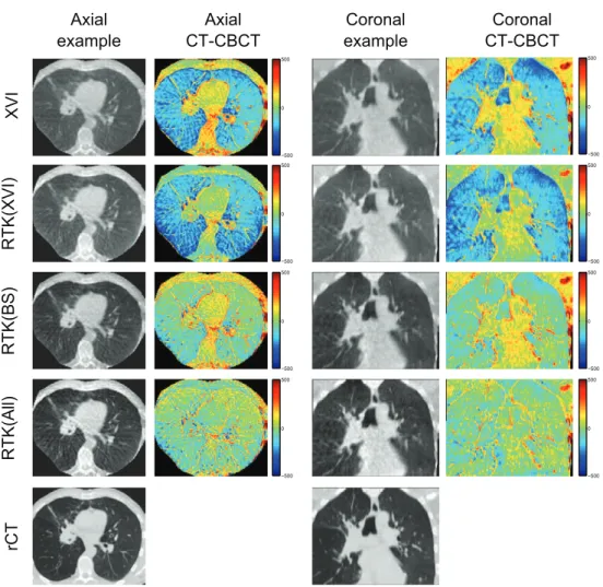
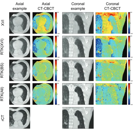
Figure 2 shows an illustrative example of axial and coronal CBCT reconstructions for patient 3. From these images, it is evident that the reconstructed CBCT HU values are too high in the lung tissues, while being too low in the tumour and bony structures on both the XVI and RTK(XVI) reconstructions. When the MC based scatter correction is applied, the HU values in the lung tissue are improved, but too low CBCT HU values in the tumour and mediasti-num remain. This remaining discrepancy is resolved when all corrections are applied in the RTK(All) reconstruction. A slight overcorrection of the bony structures is observed in the RTK(All) reconstruction. Furthermore, contrast is improved and gradients between different gray values are steeper when all corrections are applied. Example images of the remaining four patients are shown in appendix B.

The calibration plots in igure 3 show the CBCT HU values of the entire reconstructed CBCT volume as a function of the reconstructed rCT HU values for all ive patients. These plots emphasize that the XVI and RTK(XVI) reconstructions overestimate the CBCT HU values in the lung tissue, and underestimate the CBCT HU values for the bony structures.

The main difference between the XVI and RTK(XVI) reconstructions is the high CBCT HU values, where the RTK(XVI) reconstruction results in a closer match with the rCT HU values than the XVI reconstruction.

The RTK(BS) reconstructions provide a better HU match at low HU values corresponding to the lung tissue, but tends to underestimate the CBCT HU values of the soft and bony tissues. This is most pronounced for patients 1, 2, and 4, while patients 3 and 5 are nearly matched to the CT HU by the RTK(BS) reconstruction. However, when looking at the example recon-structions of patients 3 and 5 in igures 2 and B4 in the appendix, local discrepancies remain in the RTK(BS) reconstruction in the superior part of the reconstructed FOV.

When all corrections are applied in the RTK(All) reconstructions, the best one-to-one cor-respondence between the CBCT HU and the rCT HU values of the different reconstructions is found. For patient 4, igure 3 shows large CBCT HU variation in the high HU region (bony structures). This is caused by improper registration of a shoulder, and is not an effect of the Figure 2. Example images for patient 3, illustrating that all corrections are required to recover HU values in the tumour and soft tissues. The example axial and coronal images are shown with a display range of (−250 1400  ), to show contrast in the lung

tissue as well as soft tissue. Difference images are shown with a scale of (−500 500  ).

Blue colours represent too high CBCT HU values, while red colours are indicative of too low CBCT HU values compared to the rCT images.

artefact corrections. Due to the low number of voxels containing high HU values, this mis-match is very pronounced in the calibration plots.

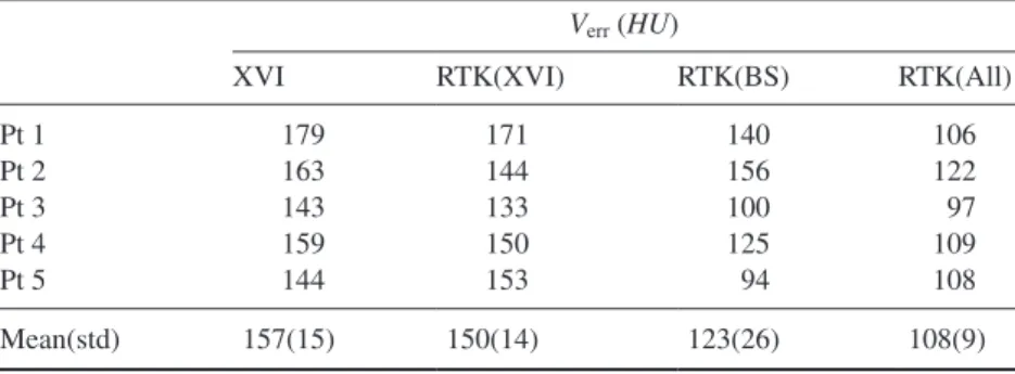
To quantify the differences in CBCT HU values, the total volume error was calculated for all reconstructions of the ive patients as shown in table 2. The overall trend is that the XVI reconstruction has the largest total volume error, with a slight decrease obtained by the RTK(XVI) reconstruction. The RTK(BS) reconstruction reduces the error further, but for four of the ive patients, the lowest HU error is found in the RTK(All) reconstruction.

Figure 3. Calibration plots for the ive lung patients displaying the median CBCT HU value as a function of the median CT HU value in 50 equidistant bins for each of the four reconstruction methods. Error bars show the 25 and 75% quartiles of the CBCT HU values in each bin. The large discrepancies at high HU values for patient 4 is due to improper registration of a shoulder.

3.1. Calculation time

Monte Carlo simulations were performed on the computer cluster in less than 2.5 h per patient. With the simulated images available, the projection image processing and reconstruction was performed in 10 min for the each patient for the RTK(All) reconstruction. Image process-ing and reconstruction was performed on the laptop PC. The extended image processprocess-ing and reconstruction time could be reduced through algorithm optimisation as well as utilisation of a higher performance computer.

4. Discussion

CBCT reconstructions of ive lung scans showed that CBCT image quality can be brought much closer to CT image quality through comprehensive artefact correction. In the present study, only postprocessing of raw projection data from our clinical database was performed. This emphasizes that the image quality improvements are achievable in any clinic that has stored their original projection data, without having to acquire new images or change their acquisition protocols.

This clinically oriented study found largest improvements in image quality when all correc-tions were applied, with the highest importance of an accurate body scatter correction method in agreement with a previous phantom study on a bench top CBCT scanner (Sisniega et al 2015). Calibration plots in igure 3 show the RTK(All) CBCT HU values scattered closely around the CT HU values, indicating that the remaining HU discrepancies after artefact corrections are ascribed mainly to image noise, as well as residual mismatch between the CBCT and rCT reconstructions after deformable registration. It is a weakness of the calibration plot analysis that some bins have a low number of voxels included, and thus become very prone to image noise and improper registration. The calibration plots must therefore be considered in relation to the example images, where the HU accuracy can be assessed in relation to the position in the image. The same sensitivity to image noise and improper registration is found in the total volume errors presented in table 2, which explains why what appears to be major changes in HU accuracy in the example images show up as only modest changes in the root mean square error metric.

The deformable registration itself is a potential source of bias favouring the RTK(All) correction on which the deformable registration was performed. We did however not observe major changes when initially investigating the registration accuracy of the different recon-structions, and the same registration was used for all reconstructions of the same patient to eliminate effects of small variations between individual deformable registration of the CBCT images in the comparison. Small anatomical variations between the rCT and CBCT recon-structions were still present although reduced through the deformable registration.

Table 2. Total volume error for the ive patients calculated according to (14).

Verr (HU)

XVI RTK(XVI) RTK(BS) RTK(All)

Pt 1 179 171 140 106 Pt 2 163 144 156 122 Pt 3 143 133 100 97 Pt 4 159 150 125 109 Pt 5 144 153 94 108 Mean(std) 157(15) 150(14) 123(26) 108(9)

The main cost of the improved HU correspondence is an apparent increase in image noise. The clinical images contains statistical Poisson noise, and when the proposed image cor-rections are applied, signal is subtracted from the clinical images. This process leads to a decreased signal to noise ratio in the projections, resulting in decreased signal to noise in the reconstructed images. Other studies have proposed the use of iterative reconstructions to combat the statistical noise (Sidky and Pan et al 2008, Tang et al 2009), and the noise could also be reduced by a post-reconstruction ilter (e.g. median iltering).

In CBCT imaging of the lungs, cardiac and respiratory motion cause blurring and streak-ing in reconstructed 3D images. These motion related artefacts are not considered in the pre-sent study, but at the same time they are not believed to cause major degradation of the effect of the proposed corrections. The image lag and detector scatter corrections simply correct for effects in the detector which are not affected by motion, while the patient speciic correction for body scatter is a spatially slowly varying function. This means that the small changes in anatomy related to the breathing motion will not have a major effect on the body scatter correction. The motion itself was not considered in the presented correction methods, but motion artefacts can be reduced through iterative reconstruction methods (Leng et al 2008) or motion compensated reconstruction (Rit et  al 2009). In addition to the motion induced artefacts, streaks arise from the undersampled CBCT acquisitions, which do not fulil Tuy’s data suficiency condition due to the circular orbit of the gantry mounted CBCT scanner (Tuy 1983).

While the present study relies on Monte Carlo based body scatter corrections, alternative options have been proposed in the literature. Suggestions of adding an anti scatter grid to the detector (Sisniega et al 2013, Stankovic et al 2014) or a stationary or moving beam blocker close to the source (Wang et al 2010, Niu and Zhu 2011, Ouyang et al 2013, Ritschl et al

2015) have shown promising results, but post-processing such as the algorithmic methods proposed by (Bertram et al 2005, Zhao et al 2015) or MC based methods (Poludniowski et al

2009, Bootsma et al 2015, Xu et al 2015) have the advantage of being able to retrospectively correct for body scatter in images of patients who already completed treatment. This makes the algorithmic or MC based approaches such as the present model more appealing for doing retrospective research on larger patient cohorts.

The scaling factor K applied prior to reconstruction of the RTK(BS) and RTK(All) was determined from the MC simulations of primary and scattered radiation. The same scaling factor could potentially be measured on the XVI system as the open ield signal, but this is not a feasible option for retrospective data analysis as the acquisition protocols may have changed. Furthermore, we have observed some variations in the output of the x-ray source when using the same preset on the same unit, and hence we favour the MC based estima-tion of K.

A different way of obtaining accurate HU in CBCT images has been proposed by Yang et al (2007) and Zhang et al (2015) where the planning CT is deformably registered to the daily CBCT. This approach has the strength of providing true HU values as long as the anatomy does not change too much, but the accuracy of the method depends on the accuracy of the deformable image registration which is dificult to validate. Furthermore, anatomi-cal changes are frequent in lung cancer patients (Møller et al 2014), and it is not clear how the deformable image registration handles the appearance or disappearance of atelectasis or pleural effusion. While the proposed MC based scatter correction based on the planning CT image will also be affected by these anatomical changes, the scattered radiation will be less sensitive to anatomical changes than the primary radiation. In the same way, small variations in patient setup between planning CT and CBCT acquisition might have a slight detrimental effect on the scatter correction accuracy. Although the present study does not correct for

these setup variations, the smooth variation in the scatter signal as well as small setup correc-tions (⩽1 cm) means that this is not expected to be a major problem.

The relative effect of each of the proposed artefact correction steps was found to be related to the individual patient rather than a common measure. The present study did not have the power to fully investigate the image quality improvement found from all potential combinations of the artefact corrections, which requires many more patients to provide a statistical measure of whether all corrections are required to obtain a signiicantly better image quality.

It is noted that a recent upgrade of the XVI software (R5.0) contains so-called HU-calibration which was not used in the clinical reconstructions in the present work. This clinically avail-able HU calibration relies on post-reconstruction linearisation of the measured grey values as measured from a phantom. For patient sizes the same as the calibration phantom this method may be relatively accurate. We do however note that a change in body scatter will cause a change in HU even after calibration, and hence the method remains to be proven accurate for patients of different sizes.

How to best evaluate image quality remains an open question with many answers depend-ing on the intended use of the images studied. Phantom studies have the strength of providdepend-ing a ground truth image since the geometry and material composition of the phantom is known, but phantoms suffer from non-realistic discontinuous density interfaces and truly homogene-ous materials, which are never found in patients. Furthermore, clinical CBCT imaging of lung cancer patients includes respiratory and cardiac motion far more complex than what can be simulated by 4D phantoms. Therefore, we believe that patient imaging can only truly be optimised on patient images.

The main use of CBCT image is for image guidance, and it is well established that even undersampled CBCT images can provide accurate image registration against the planning CT image (Westberg et  al 2010). The main driver behind the quest for improved CBCT image quality is therefore not the improvement of image registration accuracy, but rather the potential extended uses of CBCT images acquired on a daily basis. In this study, a very generic image quality measure was chosen, namely the HU resemblance of CBCT images to reference CT images. We believe that if CBCT images can provide proper HU values without severe artefacts, the potential routine uses of such CBCT images include dose calculations for treatment veriication, dose accumulation, and treatment adaptation, but also the extraction of anatomical biomarkers during the fractionated treatment course which might allow a much higher degree of personalised radiotherapy than what can be offered today.

5. Conclusion

A comprehensive artefact correction method for clinical CBCT images of the chest has been demonstrated to improve CBCT-CT HU correspondence for ive lung cancer patients with CBCT images acquired for IGRT. This study shows the irst clinical results on how sophis-ticated body scatter corrections do not sufice in realising the best image quality. To realise the best HU correspondence, all the proposed corrections must be applied in conjunction. No patient speciic optimisation of the artefact corrections was applied, and the artefact correc-tion methods work as retrospective processing of the clinical projeccorrec-tion data already available. With the improved CBCT image quality, CBCT images might have the potential to be used for dose calculation and accumulation, plan adaptation, and biomarker extraction in the same way as CT images.

Acknowledgments

CB, RST, and UB acknowledge research support from Elekta Ltd. RST acknowledges PhD funding from Odense University Hospital and CIRRO—The Lundbeck Foundation Center for Interventional Research in Radiation Oncology and The Danish Council for Strategic Research. CB and OH acknowledge support from AgeCare (Academy of Geriatric Cancer Research), an international research collaboration based at Odense University Hospital, Denmark.

Appendix A. Details of Monte Carlo simulation of the XVI source

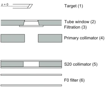
This appendix describes the simulation setup used to simulate the XVI source in the pres-ent work. Geometrical details are estimated from information found in the technical data x-ray tube housing assembly document from Dunlee, describing the DA10 series tube hous-ing (available at www.dunlee.com/resources/category/1/1/2/3/documents/DA%2010%20 Series%200309%20Dunlee.pdf on 18 April 2016), and the Technical data DU 694 x-ray tube document (www.dunlee.com/resources/category/1/2/5/5/images/DU%20694%201205.pdf, available on 18 April 2016), as well as the XVI R4.5 and R5.0 instructions for use by Elekta Ltd. Furthermore, non-destructive measurements of the x-ray source assembly was performed. It is noted that the described simulation geometry has only been estimated from measurements and information in the provided sources, and validated to give simulations which are similar to measured data. The geometry is thus not an accurate picture of the x-ray source assembly, but rather an empirical estimate which provides simulation results with suficient accuracy for the intended scatter correction purpose. While some numbers are given with high accuracy in the following description, this relects only the numbers which have been used in the actual simulation and not the accuracy with which the details are known. Most of the geometry speciications have been calculated based on speciications of ield size etc.

Figure A1 shows a schematic overview of the Monte Carlo simulation setup when simu-lating the XVI source. The source was simulated as a compiled BEAMnrc source input to egs_cbct using a photon low energy threshold of 1 keV and an electron low energy thresh-old of 512 keV (total energy).

A.1. X-ray target

The x-ray target was simulated using the XTUBE component module in BEAMnrc, with the target deined as a 5 mm thick alloy composed of 90% tungsten and 10% rhenium by weight, giving a mass density of 19.4 g cm−3_{. The target alloy was mounted on a molybdenum holder.}

The target angle was 17.5°, and the z-extend of the target was estimated to 1 cm. The cen-treline of the x-ray target was deined as the reference plane with z = 0.

A.2. Tube exit window

The tube window was simulated using the PYRAMIDS component module to deine the aper-ture of the Dunlee x-ray tube housing. The window was positioned at an estimated z = 5.73 cm, with a square aluminium window of 1.6 mm thickness and side length 2.64 cm. The Al win-dow was placed in the opening of a 3.2 mm lead block, and the opening was focused towards the focal point of electrons on the x-ray target.

A.3. Filtration

Additional iltration was simulated using the SLABS component module placed immediately after the tube exit window at z = 6.05 cm. The iltration was composed of 0.1 mm copper and 2 mm aluminium.

A.4. Primary collimator

The primary collimator in the XVI tube assembly was simulated using the PYRAMIDS component module. An unfocused square aperture with an estimated side length of 3 cm was deined in a 3.2 mm thick lead block placed at z = 6.5 cm.

A.5. S20 collimator

The S20 collimator cassette used in the present study was simulated using the SLABS, PYRAMIDS, and SLABS component modules. The S20 collimator is constructed as a lead aperture placed between two sheets of a transparent plastic material. This plastic was simulated as PETG (C10H8O4, density 1.27 g cm−3). The irst PETG slab was placed at z = 19.89 cm,

and with an estimated thickness of 1 mm. This was followed by the square collimator speci-ied using the PYRAMIDS component module, creating a 5.67 cm square opening in a 3.2 mm thick lead block. The aperture was then followed by another PETG sheet of 1 mm thickness.

A.6. F0 ilter

The F0 ilter simply consists of two plastic sheets with air in between. This was simulated using the SLABS component module with three layers placed at z = 21 cm. The irst layer was 1 mm PETG followed by 3 cm air, and inally a 1 mm PETG layer.

Figure A1. Schematic overview of the Monte Carlo simulation setup for the XVI tube. Figure not to scale.

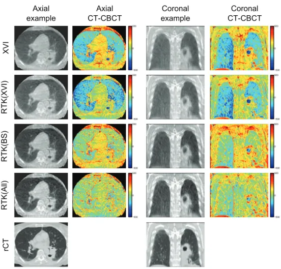
Appendix B. Example images of patients 1, 2, 4 and 5

Figure B1. Example images for patient 1. The irregular shape of the axial CBCT FOV is a result of the deformable image registration. The example axial and coronal images are shown with a display range of (−250 1400  ), to show contrast in the lung tissue as

Figure B2. Example images for patient 2. The example axial and coronal images are shown with a display range of (−250 1400  ), to show contrast in the lung tissue as well

Figure B3. Example images for patient 4. The example axial and coronal images are shown with a display range of (−250 1400  ), to show contrast in the lung tissue as well

References

Bernchou U, Hansen O, Schytte T, Bertelsen A, Hope A, Moseley D and Brink C 2015 Prediction of lung density changes after radiotherapy by cone beam computed tomography response markers and pre-treatment factors for non-small cell lung cancer patients Radiother. Oncol. 117 17–22

Bertelsen A, Schytte T, Bentzen S M, Hansen O, Nielsen M and Brink C 2011 Radiation dose response of normal lung assessed by cone beam CT—a potential tool for biologically adaptive radiation therapy Radiother. Oncol. 100 351–5

Bertram M, Wiegert J and Rose G 2005 Potential of software-based scatter corrections in cone-beam volume ct Proc. SPIE 5745 259–70

Bootsma G J, Verhaegen F and Jaffray D A 2015 Eficient scatter distribution estimation and correction in cbct using concurrent monte carlo itting Med. Phys. 42 54

Brink C, Bernchou U, Bertelsen A, Hansen O, Schytte T and Bentzen S M 2014 Locoregional control of non-small cell lung cancer in relation to automated early assessment of tumor regression on cone beam computed tomography Int. J. Radiat. Oncol. Biol. Phys. 89 916–23

Elstrøm U V, Olsen S R K, Muren L P, Petersen J B B and Grau C 2014 The impact of cbct reconstruction and calibration for radiotherapy planning in the head and neck region—a phantom study Acta

Oncol. 53 1114–24

Figure B4. Example images for patient 5. The example axial and coronal images are shown with a display range of (−250 1400  ), to show contrast in the lung tissue as well

Feldkamp L A, Davis L C and Kress J W 1984 Pracitcal cone-beam algorithm J. Opt. Soc. Am. A 1 612–9

Fotina I, Hopfgartner J, Stock M, Steininger T, Lütgendorf-Caucig C and Georg D 2012 Feasibility of cbct-based dose calculation: comparative analysis of hu adjustment techniques Radiother. Oncol.

104 249–56

Herman G T 1979 Correction for beam hardening in computed tomography Phys. Med. Biol. 24 81–106

Hsieh J, Gurmen O E and King K F 2000 Recursive correction algorithm for detector decay characteristics in ct Proc. SPIE 3977 298–305

Hubbell  J  H and Seltzer  S  M 2004 Tables of x-ray mass attenuation coeficients and mass energy-absorption coeficients (version 1.4) Technical Report National Institute of Standards and Technology, Gaithersburg, MD (http://physics.nist.gov/xaamdi)

Jabbour S K et al 2015 Reduction in tumor volume by cone beam computed tomography predicts overall survival in non-small cell lung cancer treated with chemoradiation therapy Int. J. Radiat. Oncol.

Biol. Phys. 92 627–33

Jaffray  D  A, Siewerdsen  J  H, Wong  J  W and Martinez  A  A 2002 Flat-panel cone-beam computed tomography for image-guided radiation therapy Int. J. Radiat. Oncol. Biol. Phys. 53 1337–49

Kawrakow I 2000 Accurate condensed history Monte Carlo simulation of electron transport. I. Egsnrc, the new egs4 version Med. Phys. 27 485–98

Kawrakow I, Mainegra-Hing E, Rogers D W O, Tessier F and Walters B R B 2011 The egsnrc code system: Monte Carlo simulation of electron and photon transport, nrc report pirs-701 Technical

Report National Research Council of Canada

Klein S, Staring M, Murphy K, Viergever M A and Pluim J P W 2010 Elastix: a toolbox for intensity-based medical image registration IEEE Trans. Med. Imaging 29 196–205

Leng S, Tang J, Zambelli J, Nett B, Tolakanahalli R and Chen G-H 2008 High temporal resolution and streak-free four-dimensional cone-beam computed tomography Phys. Med. Biol. 53 5653–73

Mail N, Moseley D J, Siewerdsen J H and Jaffray D A 2008 An empirical method for lag correction in cone-beam ct Med. Phys. 35 5187–96

Mainegra-Hing  E and Kawrakow  I 2008 Fast Monte Carlo calculation of scatter corrections for cbct images Int. Workshop on Monte Carlo Techniques in Radiotherapy Delivery and Veriication—3rd

McGill Int. Workshop (McGill Univ, Montreal, Canada, May 29–Jun 01 2007) (Journal of Physics Conf. Series vol 102)

Mainegra-Hing E and Kawrakow I 2010 Variance reduction techniques for fast monte carlo cbct scatter correction calculations Phys. Med. Biol. 55 4495–507

Møller D S, Khalil A A, Knap M M and Hoffmann L 2014 Adaptive radiotherapy of lung cancer patients with pleural effusion or atelectasis Radiother. Oncol. 110 517–22

Niu T and Zhu L 2011 Scatter correction for full-fan volumetric ct using a stationary beam blocker in a single full scan Med. Phys. 38 6027–38

Ohnesorge  B, Flohr  T, Schwarz  K, Heiken  J  P and Bae  K  T 2000 Eficient correction for ct image artifacts caused by objects extending outside the scan ield of view Med. Phys. 27 39–46

Ouyang L, Song K and Wang J 2013 A moving blocker system for cone-beam computed tomography scatter correction Med. Phys. 40 071903

Poludniowski  G, Evans  P  M and Webb  S 2009 Rayleigh scatter in kilovoltage x-ray imaging: is the independent atom approximation good enough? Phys. Med. Biol. 54 6931–42

Poludniowski  G, Evans  P  M, Kavanagh  A and Webb  S 2011 Removal and effects of scatter-glare in cone-beam ct with an amorphous-silicon lat-panel detector Phys. Med. Biol. 56 1837–51

Rit S, Wolthaus J W H, van Herk M and Sonke J-J 2009 On-the-ly motion-compensated cone-beam ct using an a priori model of the respiratory motion Med. Phys. 36 2283–96

Rit S, Oliva M V, Brousmiche S, Labarbe R, Sarrut D and Sharp G C 2014 The reconstruction toolkit (rtk), an open-source cone-beam ct reconstruction toolkit based on the insight toolkit (itk) J. Phys.:

Conf. Ser. 489 012079

Ritschl L, Fahrig R, Knaup M, Maier J and Kachelrieß M 2015 Robust primary modulation-based scatter estimation for cone-beam ct Med. Phys. 42 469–78

Roberts D A, Hansen V N, Niven A C, Thompson M G, Seco J and Evans P M 2008 A low z linac and lat panel imager: comparison with the conventional imaging approach Phys. Med. Biol. 53 6305–19

Rogers D W O, Walters B R B and Kawrakow I 2011 Beamnrc users manual, nrc report pirs-509(a)revl

Technical Report National Research Council of Canada

Rong Y, Smilowitz J, Tewatia D, Tomé W A and Paliwal B 2010 Dose calculation on kv cone beam ct images: an investigation of the hu-density conversion stability and dose accuracy using the site-speciic calibration Med. Dosim. 35 195–207

Sidky  E  Y and Pan  X 2008 Image reconstruction in circular cone-beam computed tomography by constrained, total-variation minimization Phys. Med. Biol. 53 4777–807

Siewerdsen J and Jaffray D 2001 Cone-beam computed tomography with a lat-panel imager: magnitude and effects of x-ray scatter Med. Phys. 28 220–31

Siewerdsen  J  H and Jaffray  D  A 1999 A ghost story: spatio-temporal response characteristics of an indirect-detection lat-panel imager Med. Phys. 26 1624–41

Sisniega A, Zbijewski W, Badal A, Kyprianou I S, Stayman J W, Vaquero J J and Siewerdsen J H 2013 Monte carlo study of the effects of system geometry and antiscatter grids on cone-beam ct scatter distributions Med. Phys. 40 051915

Sisniega  A, Zbijewski  W, Xu  J, Dang  H, Stayman  J  W, Yorkston  J, Aygun  N, Koliatsos  V and Siewerdsen J H 2015 High-idelity artifact correction for cone-beam ct imaging of the brain Phys.

Med. Biol. 60 1415–39

Spezi E, Downes P, Radu E and Jarvis R 2009 Monte carlo simulation of an x-ray volume imaging cone beam ct unit Med. Phys. 36 127–36

Stankovic U, van Herk M, Ploeger L S and Sonke J-J 2014 Improved image quality of cone beam ct scans for radiotherapy image guidance using iber-interspaced antiscatter grid Med. Phys. 41 061910

Starman J, Star-Lack J, Virshup G, Shapiro E and Fahrig R 2011 Investigation into the optimal linear time-invariant lag correction for radar artifact removal Med. Phys. 38 2398–411

Starman J, Star-Lack J, Virshup G, Shapiro E and Fahrig R 2012 A nonlinear lag correction algorithm for a-si lat-panel x-ray detectors Med. Phys. 39 6035–47

Tang  J, Nett  B  E and Chen  G-H 2009 Performance comparison between total variation (tv)-based compressed sensing and statistical iterative reconstruction algorithms Phys. Med. Biol. 54 5781–804

Thing R S and Mainegra-Hing E 2014 Optimizing cone beam ct scatter estimation in egs_cbct for a clinical and virtual chest phantom Med. Phys. 41 071902

Thing  R  S, Bernchou  U, Mainegra-Hing  E and Brink  C 2013 Patient-speciic scatter correction in clinical cone beam computed tomography imaging made possible by the combination of Monte Carlo simulations and a ray tracing algorithm Acta Oncol. 52 1477–83

Tukey J W 1967 An introduction to the calculations of numerical spectrum analysis Spectral Anal. Time

Ser. 25–46

Tuy H K 1983 An inversion formula for cone-beam reconstruction SIAM J. Appl. Math. 43 546–52

Vestergaard  A, Muren  L  P, Lindberg  H, Jakobsen  K  L, Petersen  J  B  B, Elstrøm  U  V, Agerbæ k  M and Høyer  M 2014 Normal tissue sparing in a phase ii trial on daily adaptive plan selection in radiotherapy for urinary bladder cancer Acta Oncol. 53 997–1004

Wang  J, Mao  W and Solberg  T 2010 Scatter correction for cone-beam computed tomography using moving blocker strips: a preliminary study Med. Phys. 37 5792–800

Westberg J, Jensen H R, Bertelsen A and Brink C 2010 Reduction of cone-beam ct scan time without compromising the accuracy of the image registration in igrt Acta Oncol. 49 225–9

Xu  Y, Bai  T, Yan  H, Ouyang  L, Pompos  A, Wang  J, Zhou  L, Jiang  S  B and Jia  X 2015 A practical cone-beam ct scatter correction method with optimized monte carlo simulations for image-guided radiation therapy Phys. Med. Biol. 60 3567–87

Yang Y, Schreibmann E, Li T, Wang C and Xing L 2007 Evaluation of on-board kv cone beam ct (cbct)-based dose calculation Phys. Med. Biol. 52 685–705

Zhang  Y, Yin  F-F and Ren  L 2015 Dosimetric veriication of lung cancer treatment using the cbcts estimated from limited-angle on-board projections Med. Phys. 42 4783–95

Zhao W, Brunner S, Niu K, Schafer S, Royalty K and Chen G-H 2015 Patient-speciic scatter correction for lat-panel detector-based cone-beam ct imaging Phys. Med. Biol. 60 1339–65