HAL Id: hal-02878130
https://hal.archives-ouvertes.fr/hal-02878130
Submitted on 22 Jun 2020
HAL is a multi-disciplinary open access
archive for the deposit and dissemination of
sci-entific research documents, whether they are
pub-lished or not. The documents may come from
teaching and research institutions in France or
abroad, or from public or private research centers.
L’archive ouverte pluridisciplinaire HAL, est
destinée au dépôt et à la diffusion de documents
scientifiques de niveau recherche, publiés ou non,
émanant des établissements d’enseignement et de
recherche français ou étrangers, des laboratoires
publics ou privés.
Correction of systematic radiometric inhomogeneity in
scanned aerial campaigns using principal component
analysis
Lâmân Lelégard, Arnaud Le Bris, Sébastien Giordano
To cite this version:
Lâmân Lelégard, Arnaud Le Bris, Sébastien Giordano. Correction of systematic radiometric
inhomo-geneity in scanned aerial campaigns using principal component analysis. XXIVth International Society
for Photogrammetry and Remote Sensing Congress, French Society for Photogrammetry and Remote
Sensing (SFPT), Jul 2021, Nice, France. pp.871–876, �10.5194/isprs-annals-V-2-2020-871-2020�.
�hal-02878130�
CORRECTION OF SYSTEMATIC RADIOMETRIC INHOMOGENEITY IN SCANNED
AERIAL CAMPAIGNS USING PRINCIPAL COMPONENT ANALYSIS
Lˆamˆan Lel´egard∗ Arnaud Le Bris S´ebastien Giordano
LASTIG, Univ Gustave Eiffel, ENSG, IGN, F-94160 Saint-Mande, France (laman.lelegard, arnaud.le-bris, sebastien.giordano)@ign.fr
KEY WORDS: Analogue Photography, Airborne Imagery, Radiometry, Orthophotomosaic, Hotspot Correction, PCA, KLT
ABSTRACT:
Orthophotomosaic is defined as a single image that can be layered on a map. The term “mosaic” implies that it is produced from a set of images, usually aerial images. Even if these images are taken during cloudless period, they are impaired by radiometric inhomogeneity mostly due to atmospheric phenomena, like hotspot, haze or high altitude clouds shadows as well as imaging device systematisms, like lens vignetting. These create some unsightly radiometric inhomogeneity in the orthophotomosaic that could be corrected by using a Wallis filter. Yet this solution leads to a significant loss of contrast at small scales. This work introduces an alternative to Wallis filter by considering some systematic radiometric behaviours in the images through a principal component analysis process.
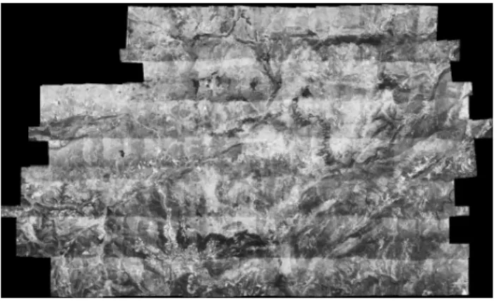
Figure 1a: Orthophotomosaic with overlaps
1. INTRODUCTION
1.1 Context
Working on former aerial campaigns has become a major issue in remote sensing and, more generally, in data sciences like for examples the European project Time Machine (Time Machine, 2019) or more local project as Swisstopo historical scanned maps (SwissTopo, 2018) and French National Mapping Agency scanned aerial campaigns available on the website IGN Remonter le Temps (IGN, 2016).
These data are interesting as they are a unique mean to access to past information about land cover. have generally be scanned by national mapping agencies and are thus available as digital data compatible with automatic processing. Thus, they open new research opportunity, for example in the studies of time varying phenomena. Yet, their exploitation leads to several geometric and radiometric processing issues. This work will specifically focus on the radiometric issues in scanned analogue airborne images. 1.2 Dataset
Datasets are only composed of images. Unlike recent aerial cam-paigns, no information about their exposure time nor the camera
∗Corresponding author.
Figure 1b: Orthophotomosaic with Voronoi cells
calibration is provided with images, yet it is here assumed that they were shot with the same camera and following the same ac-quisition pattern (Abdullah et al., 2013) which consists on several stripes, with overlaps to ensure stereoscopic analysis. Geometric processing of these images have been done using MicMac pho-togrammetric software (ENSG, 2016)(Rupnik et al., 2017): im-ages are oriented and orthorectified, making it possible to gener-ate raw orthophotomosaic renderings as shown on Figure 1.
There are many ways of mosaicking per image orthophotos, some using more advanced blending methods than others. Yet, in or-der to focus this work on image radiometric corrections, it was decided to consider only two very simple rendering solutions: using the overlaps (Figure 1a) where each pixel is the mean of the different contributing images or choosing the contribution of only one image per pixel, usually the one which the centre is the closest to the considered pixel, which leads to a Voronoi cells partition (Figure 1b).
Both rendering methods have their pros and cons: the radiometry of Figure 1a seems more homogeneous yet small shift between the different images could be observed at full resolution whereas the inhomogeneity of Figure 1b is more pronounced. In any case, both rendering are presenting radiometric heterogeneity requiring a correction step.
1.3 Existing approaches
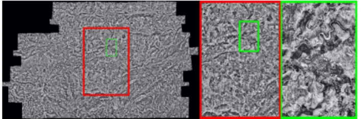
1.3.1 Statistic approaches: The image correction currently used on the historical images from IGN Remonter le Temps is purely image based and lays on Wallis filtering (Wallis, 1976) il-lustrated by Figures 2, 3 and 4. When considering Figure 2, one can notice that the contrast perception is not the same at each scale: small scales suffer from a loss of contrast whereas large scales (full resolution zoom) do not present any visible contrast alteration.
Some more recent works using Contourlet transform (Li et al., 2016) are also returning unsatisfying results when considered at small scales.
1.3.2 Multi-scales approaches: In order to perform correc-tion at different scales, one could consider multi-resolucorrec-tion blend-ing (Ogden et al., 1985) mostly used in panoramic image ren-dering (Brown and Lowe, 2007) yet requiring a preliminary vi-gnetting (image radial darkening) correction. This requirement focuses on the main issue that is here dealt with: the vignetting parameters are unknown in the present case.
1.3.3 Physical approaches: Vignetting is mostly due to two factors: the constant lens vignetting and the hotspot which could be determined by the Sun position. Knowing these parameters and using a physical model (Chandelier and Martinoty, 2009) could usually provide some relevant image corrections. Unfor-tunately, the Sun position, given by the date and the time of the aerial shot should be determined for each image, in addition of other parameters (like the aerosol composition of the atmosphere or the film response curve) that cannot be obtained on old scanned airborne missions. Consequently, physically based radiometric correction cannot be performed in our case.
2. PROPOSED APPROACH
The proposed approach is purely image based and could be come down to a Wallis filtering method regularized by all the images of a mission, the parameters of the filter being obtained by prin-cipal component analysis (PCA), also known as Karhunen-Lo`eve transform (KLT).
2.1 Wallis filtering
The principle is illustrated by the Figure 3. There are only three parameters: the size of the window, the desired mean (e.g. the mean value 128, in the case of an 8bit image) and the desired standard deviation (e.g. a value taken between 32 or 64). The mean and the standard deviation would respectively influence the luminosity and the contrast of the resulting image.
The influence of the window size is shown in Figure 4. A small window will remove the vignetting effect and all the low frequen-cies of the image whereas a large window will keep the image vignetting uncorrected. The size of the window is chosen em-pirically to obtain an acceptable compromise between vignetting correction and image legibility. In other words, this method is equivalent to calculate a gain and an offset for each pixel accord-ing to it neighbourhood.
Yet, even after having chosen manually an optimal neighbour-hood window, the final orthophotomosaic rendering is not satis-fying at small scales as shown previously on Figure 2 where large land structures are not clearly visible.
Figure 2: Wallis filter solution viewed at different scale
Figure 3: Wallis filtering
Figure 4: Wallis filtering
Figure 5: Karhunen-Lo`eve transform (KLT)
2.2 Karhunen-Lo`eve transform
This method, based on principal component analysis, is illus-trated by Figure 5. A set of vector of the same length, in the present case images represented on a canonical basis are pro-cessed to generate a new basis, called KLT basis, where most of the information is contained in the first vectors while the other vectors would give more specific information. In another way, the first vectors will show the systematic behaviours of the vec-tor set. In the case of images, they correspond to common global behaviours shared by all the images.
In this case the input vectors would be of two kind: the local mean of each aerial images and their local standard deviation (for a given Wallis filtering window chosen empirically). For each image a new local mean and a new local standard deviation are
determined using only the first vectors of the KLT basis. Using all the vectors from the KLT basis to reconstruct the local means and standard deviation would obviously lead to the initial Wallis filtering shown in Figure 2.
Principal component analysis acts here, to some extent, as a low pass filter: the first axes of the KLT basis are displaying the com-mon information somehow corresponding to low frequencies or small scales behaviour of the dataset.
2.3 Image preparation
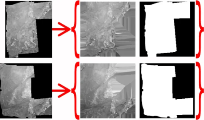
To obtain a KLT basis, the vectors, derived from the aerial or-thorectified images, should have the same length, which is not the case with the ”raw” orthorectified images from different size. In order to give all the images the same size without losing infor-mation, instead of cropping them, it was decided to include them in a bigger square frame completed by nearest neighbourhood ex-trapolation. Each new resized image is given a new mask and a new orientation file taking into account the transformation. Some examples are given in Figure 6.
Figure 6: Two extrapolated images with their associated mask
The extrapolation is justified by the fact that using directly the images with their mask would follow some irrelevant KLT basis illustrated in Appendix A.
As the phenomena that have to be corrected are related to very low frequencies, in other word very small scales, working on low resolution images is justified. In this example, considered images size is 800×800pixels.
3. RESULTS
The data set is composed of 143 orthorectified images (1.5 km footprint each) shot with an analogue camera over the Larzac area (France) in 1996. Computing the KLT basis of this set leads to 143 ”eigen” images (KLT axis) associated to respective eigenval-ues. Only the ones with stronger eigenvalues will be considered.
3.1 Choosing the relevant number of KLT axis
The choice of the ”threshold” will be empirical (yet, justified by some observations). Let’s consider the correlation of each image with the vector axis of the KLT basis of which the main axes are shown in Figure 8.
The results are shown in Figures 7. All the images are strongly correlated with the first axis: this is the main behaviour of our images set. The second axis is more interesting: two distinct behaviours are observed on Figure 7b between the North and the
Figure 7a: Correlation with the first KLT axis (local mean)
Figure 7b: Correlation with the second KLT axis (local mean)
Figure 7c: Correlation with the third KLT axis (local mean)
Figure 7d: Correlation with the fourth KLT axis (local mean)
South of the mission. After considering the eigen image relative to the second axis, this could be interpreted as a change of the
hotspot shape, probably due to a different position of the Sun.
Further investigation showed that the images were not taken the same day; it was a two days mission. The correlation with the third or fourth axis (Figures 7c and 7d) is more difficult to inter-pret: the variation seems somehow more or less correlated along one strip. The correlations on other axis do no show any struc-tured behaviour.
Figure 8: The 24 main KLT axis (local mean) sorted by their decreasing eigenvalues
So only the three (or four) first axis seem relevant to model the local means and standard deviations of each image, the other or-ders axis being not correlated with systematic phenomena that we try to remove.
3.2 Orthophotomosaic rendering
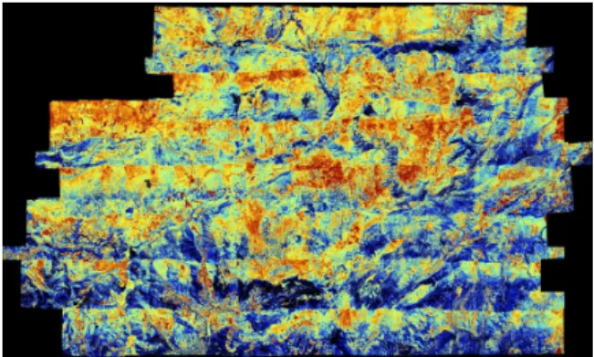
In order to compare and discuss the results in a more visual and efficient way by artificially increasing the dynamic of the images, the Figure 9 proposes a colour scale representation of the result-ing orthophotomosaics rather than a greyscale one.
Compared to uncorrected overlap rendered orthophotomosaic (Fig-ure 9a), obtained results are more homogeneous even if some lit-tle discontinuities seem to be present in their Voronoi cells render-ing shown on Figure 9c (that could be compared with the uncor-rected version given by Figure 1b). These discontinuities are al-most invisible when considering overlaps rendering (Figure 9d).
A compromise is obtained by merging the two reconstructions: in practice, applying another Wallis filter on the corrected images where the desired mean and standard deviation are no more fixed but given by the overlaps rendered orthophotomosaic: the details coming from the Voronoi cells rendering and the low frequencies from the overlaps rendering.
Eventually, the proposed method avoids the loss of contrast fol-lowing the Wallis filtering approach (Figure 9b). Yet, some initial choices could be discussed and developed.
3.3 Discussion and further developments
This method is justified by the fact that the image set is composed of a large amount of images, yet on small sets of images, this method would probably show some limits.
Also the fact orthorectified images are used instead of consider-ing directly the camera geometry images might be justified by the assumption that oriented images would give better results, yet
Figure 9a: Orthophotomosaic with uncorrected overlaps
Figure 9b: Orthophotomosaic corrected with simple Wallis
Figure 9c: Our result rendered with Voronoi cells
Figure 9d: Our result rendered with overlaps
restarting the experiment directly on the ”original” scanned im-ages before orthorectification could be an interesting alternative approach to this method. The image preparation illustrated by Figure 6 would also be much faster.
4. PERSPECTIVES
Compared to existing radiometric equalization methods, without any context information, the proposed simple approach gives bet-ter visual results. Yet, this method is only limited to panchromatic images. Applying it directly to colour images (separately on red, green and blue bands) leads to some drab and unsightly results shown in Appendix B. The colour approach should be considered in a different way, typically by first avoiding using fixed global mean and standard deviation as it is done in this work.
Another perspective would be to perform the method directly on ”raw” images (e.g. before orthorectification) and see its influence on the photogrammetric process leading to final product as digital terrain model and orthorectified images. Eventually, the last step would consist on testing our method on larger datasets, like for example a region or a whole country in order to discuss it possible limits.
REFERENCES
Abdullah, Q., Bethel, J., Hussain, M. and Munjy, R., 2013. Pho-togrammetric project and mission planning. In: McGlone, J.C.
(Ed.), Manual of Photogrammetry. American Society for Pho-togrammetry and Remote Sensing, pp. 1187–1220.
Brown, M. and Lowe, D., 2007. Panoramic image stitching us-ing invariant features. International Journal of Computer Vision 74(1), pp. 59–73. doi:10.1007/s11263–006–0002–3.
Chandelier, L. and Martinoty, G., 2009. A radiometric aerial triangulation for the equalization of digital aerial images and orthoimages. Photogrammetric Engineering Remote Sensing
75(2), pp. 193–200. doi:10.14358/PERS.75.2.193.
ENSG, 2016. Micmac.https://micmac.ensg.eu - link visited
on February the 6th, 2020.
IGN, 2016. Remonter le temps. https://remonterletemps. ign.fr - link visited on February the 6th, 2020.
Li, W., Sun, K., Li, D. and Bai, T., 2016. Algorithm for auto-matic image dodging of unmanned aerial vehicle images using two-dimensional radiometric spatial attributes. Journal of
Ap-plied Remote Sensing10(3). doi:10.1117/1.JRS.10.036023. Ogden, M., Adelson, E., Bergen, J. and Burt, P., 1985. Pyramid-based computer graphics. RCA Engineer 30(5).
Rupnik, E., Daakir, M. and Deseilligny, M. P., 2017. Micmac – a free, open-source solution for photogrammetry. Open Geospatial
Data, Software and Standards2(14). doi:10.1186/s40965-017-0027-2.
SwissTopo, 2018. A journey through time - maps. https: //www.swisstopo.admin.ch/en/maps-data-online/ maps-geodata-online/journey-through-time.html
-link visited on February the 6th, 2020.
Time Machine, 2019. Invigorating european history with the big data of the past. Time Machine, This project has received funding
from the European Union’s Horizon 2020 research and innova-tion program under grant agreement No 820323.https://www. timemachine.eu - link visited on February the 6th, 2020. Wallis, R., 1976. An approach to the space variant restoration and enhancement of images. In: Proceedings of the Symposium
on Current Mathematical Problems in Image Science, Montery, CA, USA.
ACKNOWLEDGEMENTS
This work was supported by the French National Research Agency under the grant ANR-18-CE23-0025.
...
...
APPENDIX A
...
The 99 first axes (sorted by decreasing eigen-values) of the KLT basis with (top) and without (bottom) extrapolation of the image border mask:
APPENDIX B
From top to bottom, colour orthophotomosaic rendered: with-out correction, with Wallis filtering on the RGB layer, with our method applied directly on the RGB layers:
... ... ... ... APPENDIX C ...
... More results on a smaller campaign composed of 27 images.
... ...