Cogeneration system size optimization and return on investment study

by

> wi.

-AND RETURN ON INVESTMENT STUDY

KEVIN ANDREW MAYER

SUBMITTED TO THE DEPARTMENT OF MECHANICAL ENGINEERING IN PARTIAL FULFILLMENT OF

THE REQUIREMENTS FOR THE DEGREE OF BACHELOR OF SCIENCE IN MECHANICAL ENGINEERING

a* the

MASSACHUSETTS INSTITUTE OF TECHNOLOGY

December 19, 1983

© 1983 Massachusetts Institute of Technology

Signature of Author _ 9g LL BN

Department of Meckfnical Engineering

December 19, 1983

Certified by _ ) Cs Maher El- Masri

Pan Thesis Supervisor

Accepted by” _

Chairman,

EE MASSACHUSETTS RBATIFReNt Thesis Committee

OF TECHNOLOGY

MAR 21 1984

Archives

LIBRARIES

2

by

COGENERATION SYSTEM SIZE OPTIMIZATION AND RETURN ON INVESTMENT STUDY

KEVIN ANDREW MAYER

Submitted to the Department of Mechanical Engineering on

December 19, 1983 in partial fulfillment of the

requirements for the Degree of Bachelor of Science in

Mechanical Engineering

ABSTRACT

A computer study was performed to determine optimum system sizes and

corresponding returns on investment for gas turbine cogeneration

systems located at relatively small sites. A sensitivity analysis was also performed to establish which parameters the optimum system

size and the return on investment were most sensitive to. This was

accomplished by varying one program input while holding all other inputs constant. The optimum system size was sensitive only to

(excluding energy consumption requirements) the utility electricity

prices and the utility buy-back rates. Even to these parameters,

the optimum size was insensitive until large variations were

introduced. The return on investment was most sensitive to the

utility electricity price, the price of natural gas, the marginal

tax rate, and the magnitude of financing. The return on investment

was least sensitive to the standby charge, the system lifetime,

and the inflation rate. In the absolute sense, all calculated

returns on investment were high, showing an investment in

cogeneration to be quite attractive.

Thesis Supervisor: Maher El-Masri

I would like to thank Professor El-Masri for his continuous support throughout my years at MIT, both as my academic and thesis advisor.

Thanks also to the Department of Mechanical Engineering staff and faculty. They made my experience here productive and enjoyable.

Thank you Professor Dewey for letting me use the printer.

Of course, thanks to all the brothers of Sigma Alpha Epsilon for

putting up with me all these years.

A profound thanks to my parents whose financial and moral support made possible the completion of my studies."wm St PF

lL

TABLE OF CONTENTS

2.1 Cogeneration technologies 10

2.2 Federal incentives i5 ~ Methods of analysis '8 3.1 Gas turbine characteristics 18

3.2 Optimization and return on investment 21

342.1 Optimization methodology 21

3.2.2 Net present value analysis 24

3.2.3 Return on investment analysis 27 ~~ Potential cogeneration sites £8

2,4 Input parameters oh

3.4.1 Hardware assumptions

3.4.2 Economic parameters i 3.4.3 Financial parameters = L, Analytical results ;

4.1 Size optimization and return on investment "a

4,2 Sensitivity analysis 45

4.2.1 Optimum system size Lé

5. Conclusions and recommendations be 3

5.1 Conclusions 213

5.2 Recommendations Aly

Appendix A £5

Appendix B 71

LIST OF FIGURES

Figure 2-1: Conventional Systems Compared With Cogeneration 11

Figure 2-2: Typical Simple Gas Turbine Cogeneration System

Schematic 13

Figure 3-1: Allison 501-KB Fuel versus Output 20

Figure 3-2: Optimization Analysis Algorithm 22

Figure 3-3: Energy Requirements for Battle Creek Hospital 29

Figure 3-4: Energy Requirements for San Diego Hospital “0

Figure 3-5: Energy Requirements for Lake City Hospital 21

Figure 3-6: Energy Requirements for Buffalo Hospital “2

Figure 3-7: Energy Requirements for M.I.T. "3

Figure 4-1: Cogeneration System Energy Output for San Diego

Hospital 39

Figure 4-2: Cogeneration System Energy Output for Battle

Creek Hospital 40

Figure 4-3: Cogeneration System Energy Output for Lake City

Hospital 41

Figure 4-4: Cogeneration System Energy Output for Euffalo

Hospital L2

Figure 4-5: Cogeneration System Energy Output for M.I.T. L3

Figure 4-6: NPV to Capital Outlay Ratio versus System Size

for M.I.T. Ls

Figure 4-7: Turbine Size Sensitivity for San Diego Hospital Ly

Figure 4-8: Turbine Size Sensitivity for Buffalo Hospital "8

Figure 4-9: Turbine Size Sensitivity for Lake City Hospital L9

Figure 4-10: Turbine Size Sensitivity for Battle Creek

Hospital 50

Figure 4-11: Turbine Size Sensitivity for M.I.T. 51 Figure 4-12: ROI Sensitivity to Fardware and Economic Variables

for Buffalo Hospital 53

Figure 4-13: ROI Sensitivity to Hardware and Economic Variables

for Lake City Hospital 51

Figure 4-14: ROI Sensitivity to Hardware and Economic Variables

for San Diego Hospital 55

Figure 4-15: ROI Sensitivity to Hardware and Economic Variables

for Battle Creek Hospital 56

Figure 4-16: ROI Sensitivity to Hardware and Economic Variables

for M.I.T. 57 Figure 4-17: ROI Sensitivity to Tax and Financing Variables for

Buffalo Hospital 58

Figure 4-18: ROI Sensitivity to Tax and Financing Variables for

Lake City Hospital 59

Figure 4-19: ROI Sensitivity to Tax and Financing Variables for

San Diego Hospital 60

Figure 4-20: ROI Sensitivity to Tax and Financing Variables for

Battle Creek Hospital 61

Figure 4-21: ROI Sensitivity to Tax and Financing Variables for i

4

LIST OF TABLES

Table 2-1: Summary of Gas Turbine Technology 14

Table 3-1: Summary of Input Parameter Values 36

CHAPTER ONE

INTRODUCTION

1.1 Historical perspective

Cogeneration, as a concept and a practice, is not new. During the late 1800s and early 1200 s various types

of cogeneration technologies were developed in Europe and the United States. Cogeneration was particularly

attractive in that period because utility produced

electricity was unreliable and expensive. As the twentieth

century progressed, and utilities became extremely

reliable and less costly under heavy regulation, the interest in on-site electricity production declined.

Concomitantly, the number of sites in the United States which had electrical and thermal loads suitable for

cogenerated energy increased. Due to this, and the increased awareness of energy costs, there is now a renewed interest in cogeneration as a viable energy

alternative.

1.2 Benefits of cogeneration

Cogeneration is the simultaneous on-site production

8

using one prime mover. Thus the exhaust heat which is generated as a by-product of the production of electrical power is recaptured and used for thermal energy

requirements. This simultaneous production costs less than the combined costs of utility purchased electricity and

on-site steam production. The nature of this dual production process is to increase the overall fuel

efficiency of the energy production process. This results

in aggregate national fuel savings and in a more global

sense a decreased reliance on foreign energy sources.

1.3 Goals and structure of this study

This report examines the effects of various economic

and technological parameters on the optimal cogeneration

system size and on the internal rate of return for the

cogeneration system investment for a given site. A

potential site is characterized by both the sites energy

requirements and the economic environment in which it is

situated. One goal of this study is to predict an optimum

cogeneration plant size for different potential

cogeneration sites which differ in energy consumption

profiles and in their economic situations. Another goal is

to calculate the return on investment for the cogeneration

systems corresponding to optimum system sizes, as well as

to determine the sensitivity of the system size and the

effect of uncertainties in these parameters on investment

decisions can be determined.

Chapter 2 begins with a discussion of cogeneration technologies and goes on to address Federal cogeneration incentive policies. Chapter 3 introduces the methods of analysis used for the optimization and internal rate of return algorithms. Chapter 4 presents the results of the study and briefly discusses and analyzes these results. Chapter 5 concludes the report and suggests future

10

CHAPTER TWO

OVERVIEW

2.1 Cogeneration technologies

Cogeneration technologies can be broken down into two

major sub-catagories, topping cycles and bottoming cycles.

power first and then produce thermal power: these are the

most common types of cogeneration systems. Conversely,

bottoming cycle systems produce thermal power first and

then produce electricity, and are much less common than

topping cycle systems. As previously pointed out,

cogeneration systems are more efficient at producing both thermal and electrical power than are systems which

produce only steam or only electricity, as Figure 2-1

illustrates.

The following are some of the more common types of cogeneration technologies along with their most practical

applications. The steam turbine topping cycle can vary in size from about 500 kW to 100 MW and can run on natural gas, distillate, residual fuels, coal, wood and a variety

of other fuels. This system can be expected to have a lifetime of about 25 to 35 years and is the most commonly

YIEAY

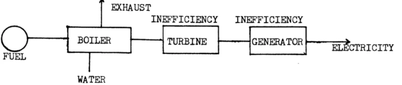
Figure 2-1 : Conventional Systems Compared With Cogeneration

| EXHAUST INEFFICIENCY INEFFICIENCY o : Tm m— .

a TURBINE GENERATOR =—

A) Conventional electrical requires 1 barrel of oil to produce 600 kWh

| EXHAUST

- sr INDUSTRY; R

sora B ' PROCESS

= ;

FUEL WATER

B) Conventional process-stean requires 2.25 barrels of oil to produce

8500 lbs. of process steam

# EXHAUST

| INEFFICIENCY INEFFICIENCY

— |Borie TURBINE GENERATORF— —3 ELECTRICITY

STEAM JProcess

FUEL a

C) Cogeneration system requires the equivalent of 2.75 barrels of oil to

SOURCE: Office of Technology Assessment, Industrial and Commercial

12

Hx).

utilities, or in any application where the electric to

thermal enrgy requirement ratio is low. The open cycle gas

turbine is available in sizes ranging from 100 kW to 100

MW and is commercially available in large quantities, being a mature technology. This system can run on a variety of fuels including natural gas, distillate,

treated residual /coal, or biomass—derived gases and

liquids, although it is best suited to natural gas and low—sulphur oil. The open cycle gas turbine cogeneration system is well suited for use in residential , commercial.

and industrial sectors given the proper economic

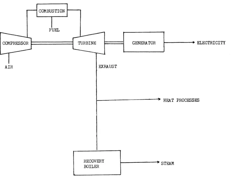
conditions. This system was chosen for this study, and is sketched schematically in Figure 2-2. A summary of the gas

turbine characteristics can be found in Table 2-1.

The diesel topping cycle is another mature technology which is available commercially in large quantities. It has a size range from 75 kW to 30 MW. Because of its

reliability and availibility, the diesel topping cycle can

be used in hospitals, apartment complexes, shopping

centers, hotels, and a host of other applications. Other

technologies currently being developed and deserving

mention are the closed-cycle gas turbine cycle, the

combined gas turbine/steam turbine topping cycle, the fuel

cell topping cycle, and the Stirling engine topping cycle,

all of which show promise for the future (Office of

FI

. COMPRESSOR {———————-=% TURBINE I————— GENERATOR ELECTRICITY

A EXHAUST

HEAT PROCESSES

RECOVERY —

BOILER oe

Figure 2-2 : Typical Simple Gas Turbine Cogeneration System Schematic

SLL

IR

14

Table 2-1 : Summary of Gas Turbine Technology

'" Unit size: 500 kW - 100 MW

Fuels: natural gas, distillate, treated residual/coal, biomass

derived gases and liquids

Average annual availability: 90-95 %

Full load electric efficiency: 24-35 %

50 % load electric efficiency: 19-29 %

Electricity to steam ratio: 140-225 kWh/MMBTU

Total installed cost: 320-700 $/kW

Construction lead time: 0.75-2 years

Expected lifetime: 20 years

Commercial status: mature technology, available in large

quantities

Applicability: residential, commercial, industrial

SOURCE: Office of Technology Assessment, Industrial and Commercial

2.2 Federal incentives

The bulk of the Federal incentives for cogeneration

are promulgated in the Public Utilities Regulatory

Policies Act of 1978 (PURPA). Because it has been shown that the United States wastes about the same amount of

energy that it imports (Dames and Moore, 1981), the

Federal government regards energy conservation as an

important national priority, as PURPA clearly

demonstrates. Basically, PURPA (Section 210) requires the Federal Energy Regulatory Commission (FERC) to establish

policies to encourage cogeneration.

PURFA Section 210 mandates the following important Federal cogeneration policy incentives. Section 210

assures that utilities may not price cogeneration back-up

electricity discriminatorily, and that qualifying

cogenerators receive prices for power sales to electric utilities which are just and reasonable, and in the public interest. This "buy-back" provision has been hotly

contested in the courts the past few years, but recently

the U.S Supreme Court decided that the FERC was correct in

ordering utilities to pay cogenerators the utilities” full

avoided costs for any electrical power purchased {from

qualified cogenerators. The decision also upheld an FERC

policy that utilities must effect an interconnection with any small power producer that warrants one, without

16

1983.

full-scale evidentiary hearings (The Energy Dailv, ¥ The advantages of this decision for qualifying

cogenerators are obvious. The price utilities must pay for

electrical power is completely independent of the

cogenerator™s power production cost. Additionally, cogenerators are assured a market for any excess

electricity produced, and are also assured reasonable interconnection costs.

Other pieces of legislation provide incentives to potential cogenerators. The Industrial Fuel Use Act of

1978, which limits the use of oil and natural gas contains

some special exemptions for cogenerators. The Natural Gas Policy Act of 1978 protects cogenerators from the normal

incremental gas pricing policies, and thus saves money for

qualifying cogenerators in several regions. The Energy Tax

Act of 1978 provides tax incentives for cogenerators. Under the specially defined and alternate energy property provisions of the Act, some components of cogeneration

property are entitled to additional tax credits beyond the

usual 10 percent investment tax credit. Finally, the Economic Recovery Tax Act of 1981 places cogeneration equipment under accelerated cost recovery system (ACRS) five year business property which allows full depreciation

of equipment in a five vear period.

This enacted legislation makes obvious the Federal

1 this country. The Office of Technology Assessment makes further recommendations for additional policy concerning cogeneration. OTA feels that future policy should be directed towards reducing oil use in future systems by introducing extra incentives for non—-oil fired systems.

OTA further suggests that utility owned cogeneration

systems be entitled to equal benefits under the law. Another suggestion is to reduce the air quality

regulations for cogenerators due to their increased fuel

efficiency. These policy measures would make an investment in cogeneration systems even more attractive in the future and reduce the overall oil consumption in this country.

18

CHAPTER THREE

METHODS OF ANALYSIS

This chapter presents the methodology used for the

system size optimization and return on investment analyses. A computer program was written at the Joint

Computer Facility at M.I.T. to accomplish these analyses,

a copy of which can be found in Appendix A. A sample

output is located in Appendix B. The determination of the

input parameters used to run the program is discussed

later in the chapter.

3.1 Gas turbine characteristics

As cited earlier, the gas turbine topping cycle was

chosen as the prime mover for this analysis. This system was chosen because of the typical system size

requirements, the thermal and elctric load profiles of the sites considered, reliability, and maintenance

characteristics.

Many of the quantitative characteristics of gas turbine systems were taken from Cogeneration and Utility Planning, FPickel’s 1982 doctoral thesis. Pickel estimated the capital cost for gas turbine cogeneration systems to

follow a logarithmic function of the electric output

capacity. This 1980 equation has been increased here by 30 percent to account for the past three years of inflation

to produce the following:

CCqp = 1660 - 120 1n E, 3.1)

where CCqrp is the capital cost for the turbine in 1983

dollars, and Eq is the turbine’s electrical output

capacity in kilowatts. This relation accounts for the price of the turbine, installation, and all necessary

auxilliary systems and engineering efforts.

An equation for the rated output turbine electric efficiency was also taken from Pickel, but multiplied by a

factor to approximate the electric efficiencies of a

modern Allison gas turbine model. Rated output gas turbine

electric efficiency is given by:

Te =T+exp(1.3588=0.1079Tn55)£32)

where oo is the turbine’s maximum electrical output in

megawatts.

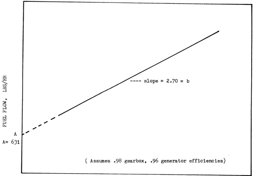
To predict the attenuation of the electric efficiency when the gas turbine operates below its maximum capicity, the performance charateristics of a typical gas turbine

(in this case an Allison model S501-KRBR) was used (see Figure 3-1). From the linear relationship between fuel

& 3 3 { "pe = 2.70 = b

q

=.

=

A= 631 |

. Assumes .98 gearbox, .96 generator efficiencies)

GENERATOR OUTPUT, KW

Figure 3-1 : Allison 501-KB Fuel versus Output

31C..

and:

following relationship for the electric efficiency of the

gas turbine operating at less than rated output was

derived:

7 _ 1 (1 - v7)g Max) (A + b-CAPMAX) (3,3)

E,ACT b b (A + b-PCAP:CAPyAX) |

where b is the slope of the fuel versus output curve, A

is the intercept of the same curve in kilowatts, CAP, y is the rated operating capacity of the turbine in kilowatts, and PCAP is the decimal coefficient which

represents the capacity at which the turbine is operating: Actual operating capacit

PCAP = ~ Sperating capacity | (3.4)

Rated operating capacity

Ne =: Moi Dan (3.5)

where Nex is the gearbox efficiency, 7) cEN is the

generator efficiency of the gas turbine system, and 7]

3.2 Optimization and return on investment

3.2.1 Optimization methodology

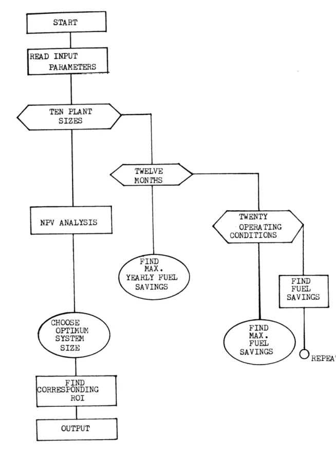
The algorithm used for the optimization portion of

the analysis is shown in flowchart form in Figure 3-2. Ten potential gas turbine sizes were considered, the size

being described by the turbine’s rated electrical output capacity. The smallest size considered was that size just

22

, 2 2X aL

Figure 3-2 : Optimization Analysis Algorithm

STA RT |

PARAMETERS |

SIZES /

agenteens

TWENTY

Eg mo

SYSTEM a

Biz SAVINGS A

> REPEAT

ROI i

—

OUTPUT |

1 yo

-able to meet one half of the lowest average site monthly

electrical power requirement; the largest size considered

was just able to meet twice the lowest average electrical

power requirement:

CAP, = 0.5 ELREQy 1 3 CAF, x = 2 ELREQy 1x (3.6)

where CAP is the size of the turbine, and ELREQ,Tn is the lowest average electrical power requirement.

For each turbine size, the turbine was then taken to

operate at twenty different capacities for each month, so that PCAP as defined in equation (3.4) ranged from:

a . = ° ( °

PCAPy, r= 0.2 PCAPy,y=1.0(3.7)

Thus the turbine was run from 20 percent of its rated

capacity to 100 percent of its rated capacity for each

month and for each of the ten turbine sizes. The

electrical efficiency was then determined using

equation(3.3). For each operating condition, the

electrical power output was calculated by:

ELOUT = PCAP:'CAP 3.8)

where ELOUT is in kilowatts. The fuel needed to operate

the cogenerator at this point is given by:

J = * . / °

FUEL (BLOUT/ Tg op) 2l4.- 30 3.9)

24

corresponding thermal output was calculated using:

THOUT = FUEL (1 -T];) BOIEFF:0.97 (3.10)

where THOUT is in kilowatt-hours per month which is

easily converted to BTU per month, BOIEFF is the boiler efficiency, and 0.97 accounts for turbine losses.

Once ELOUT and THOUT were determined for a particular

PCAFP and month, the monthly fuel savings were found by

comparing the cogeneration outputs to site energy demands,

noting that any excess electricity produced was bought

back by the utility at the legally established buy-back

rate. The fuel savings were then calculated as the fuel

cost without the cogeneration system in place less the total fuel cost with the cogeneration system. For each

month, the turbine operating condition which yielded the

greatest fuel savings was chosen as the optimum operating

condition. In this manner, a maximum yearly fuel savings

and a corresponding optimum operating profile (by month)

was established for each of the ten considered turbine

sizes. Each turbine size, with its corresponding capital cost (equation (3.1)) and its corresponding maximum yearly

fuel savings were then inputs to a net present value (NFV)

analysis to choose the optimum turbine size.

2.2.2 Net present value analysis

cogeneration system can be expressed: 2 NETSAV

NPV = — Y__)}—CAPCOS(3.11)

x (1 + 5)

where Y is the lifetime of the equipment in years, NETSAV,

is the net savings in year y , CAPCOS is the initial

capital outlay at the time of the purchase (year zero),

and DR is the discount rate of money. A look at the components of equation (3.11) is now in order.

Capital cost. CAPCOS represents the total initial

capital cost of the system less any tax credits and less

any borrowed capital, thus:

CAPCOS = CCqp (1 - ITC - EITC - FIN) + ICN-CAP (3.12)

where ITC represents the investment tax credit ( i.e.,

for a ten percent investment tax credit, ITC equals 0.10) ,EITC represents the energy investment tax credit, and FIN

represents the percentage of capital cost borrowed, as a

decimal quantity.

Net savings. The net savings in year y can »>e

expressed:

NETSAV,= (1 - TR) (1 + GR)” (FUESAV, - Omg) + (3.13)

TR +DEPy (CC (1 - 0.5 ITC - 0.5 EITC) + ICN+CAP)

where Tk is the decimal equivalent of the marginal tax rate, GR is the decimal annual growth rate of fuel and maintenance costs, FUESAV,4 is the fuel savings in year one, OMq is the operation and maintenance cost in year

26

one, ICN is the cost of utility interconnection in

dollars per kilowatt of installed capacity, and DEPy is

the depreciation coefficient in year y . If financing is

considered, equation (3.13) is ammended to:

NETSAV_ = (1 - TR) (1 + GR)Y (FUESAV, - OM, ) - ALP,

TR (DEPy ( CCyyp (1 - 0.5 ITC - 0.5 EITC) + 3.14)

ICN-CAP) + LIP}

where LIP is the loan interest payment in year y and ALF

is the total annual loan payment in year

Depreciation. Under the new accelerated cost recovery

system, ACRS, the cogeneration equipment is eligible for complete depreciation under the following yearly

coefficients:

DEP1 = 0.15 : DEP2 = 0.22 ; DEP3 = 0.21 ; DEP4 = 0.21

DEP5 = 0.21 ; DEP6—= 0.0 (3.15)

Note that DEP1 + DEP2 + DEP3 + DEP4 + DEPS = 1.0.

Financing. For financing the capital cost, a repayment schedule in which an equal portion of the principal is paid back in each year in addition to

interest on the unpaid balance of the principal was

considered. Under this repayment plan, the annual loan

payment 1s:

ALP, =P (1/N+ (1 -(y-1)/N) IR) ex N (3.16)

where P is the total principal borrowed, N is the loan repayment period, and IR is the loan interest rate. The

loan payment less the amount of principal repaid:

LIP, = P (1 - (y -1)/N) Ir we N (3.17)

From the above equations, a net present value for each of the ten different possible turbine sizes was

calculated. However, since capital for these investments would probably be scarce, the optimum plant was chosen by the highest return on investment, not by highest net

present value. After the net present value was calculated,

the ratio between the net present value and the

corresponding initial capital outlay was found. Because

the internal rate of return is an increasing monotonic

function of this ratio, the plant with the highest ratio was chosen as the input to the return on investment

analysis, and was considered optimum.

3.2.3 Return on investment analysis

This part of the analysis used as its inputs the

size, capital cost, and net savings of the plant size

which was found to have the highest NPV to capital outlay ratio. The return on investment is simply that discount

rate in equation (3.11) which drives the net present value to zero. Thus the same equations govern this analysis as governed the net present value analysis, and will not be

28

determination of the return on investment for the optimal

system size operating at its optimal capacity each month.

A sensitivity analysis was also performed by varying one parameter while holding all others constant to determine which parameters the rate of return and the optimum system size were most sensitive to.

3.3 Potential cogeneration sites

Five sites were chosen as potential cogeneration facilities for this study. Four of these sites are

hospitals spread throughout the country in different economic and environmental conditions. These sites were

chosen because of the availability of their energy

consumption data. their geographical spread. and their

differing economic parameters. The Veteran’s

Administration operates three of the hospitals: those located in Buffalo, New York: Lake City, Florida: and San

Diego, California. The fourth hospital is located on a

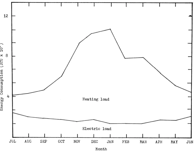
military post in Battle Creek, Michigan. The heat and

electric requirements for these sites were obtained from

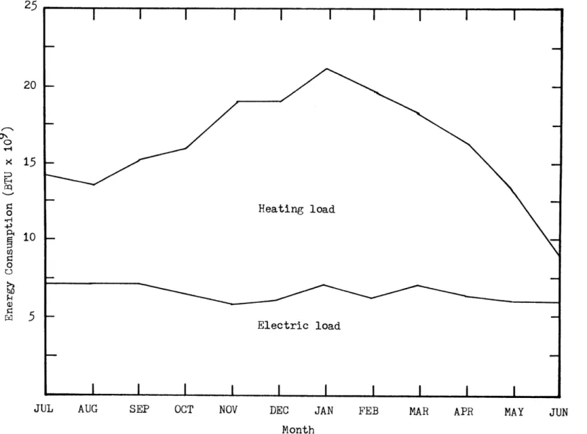
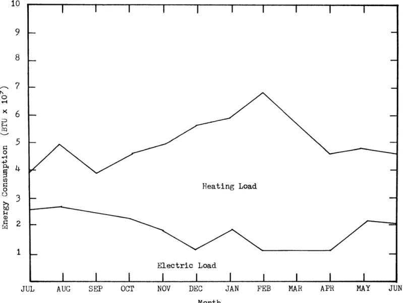
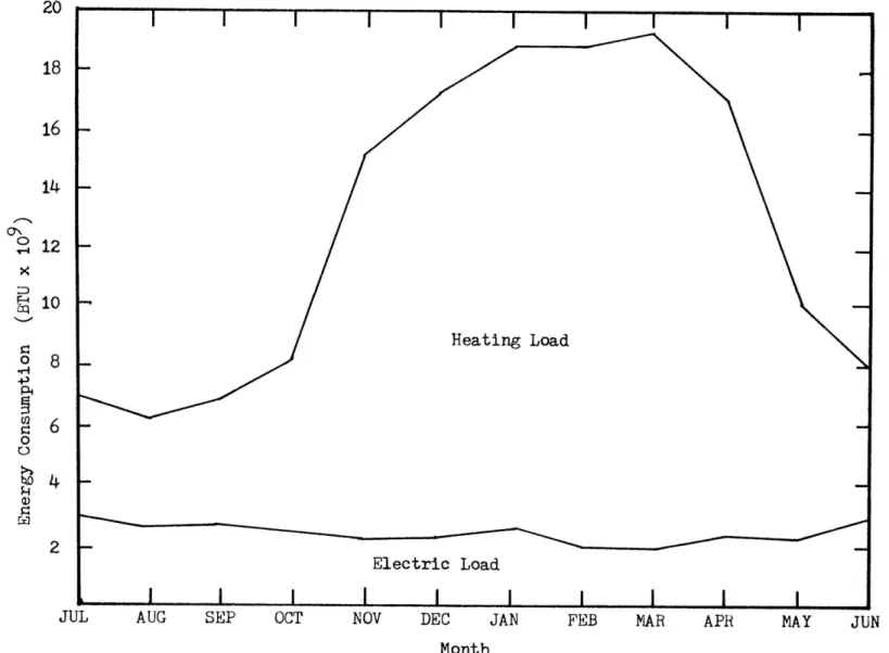
Flint’s 1983 thesis, and are depicted graphically in Figures 3-3 through 3-6. The fifth potential site chosen

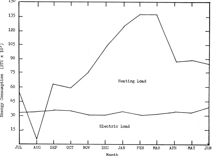
was the Massachusetts Institute of Technology because it is not a hospital like the other sites and therefore has different energy requirements, its heat and electrical loads (Figure 3-7) were readily available from the

LA

Heating load

Electric load i

—_— rrpr1Ji

JUL AUG SL. OCT NOV DEC JAN FEB MAR APR MAY JUN

Month

Figure 3-3 : Energy Requirements for Battle Creek Hospital 17

iL

Rn

TTT fTTTT=

; Heating load

= 10 kL

Month

Figure 3-4 : Energy Requirements for San Diego Hospital

wed

~~

c } f i

: Heating Load

I

5

5

| I | : | | I | |

JUL AUG SEP OCT NOV DEC JAN FEB MAR APR MAY JUN Month

Figure 3-5 : Energy Requirements for Lake City Hospital

«

7 ” - : TT T 7 TT pre

12 +

1

I

5 10 |

Heating Load

Ly

JUL AUG oEP OCT NOV DEC JAN FEB MAR APR MAY JUN Month

Figure 3-6 : Energy Requirements for Buffalo Hospital

a“

wa) nd

135 bo

120 }—

9 |.

:

75

- Heating Load

S60

wl

-CL J yo

JUL AUG SEP OCT No DEC JAN FEB MAR APR ‘MAY JUN Month

Figure 3-7 : Energy Requirements for M.I.T.

x

Bad

physical plant office, and it was of personal interest to

the author.

3.4 Input parameters

This section presents a brief discussion concerning

the values of the important input parameters of the

analysis program.

3.4.1 Hardware assumptions

All boilers were reasonably assumed to be 80 percent

efficient. The slope and intercept of the gas turbine fuel versus output curve (Figure 3-1) were obtained from

Allison model S501-KR literature, and are probably

representative of most gas turbines. The lifetime of the

cogeneration system was conservatively assumed to be 15

vears. The operation and maintenance costs were assumed to

be 10 percent of the turbine capital cost yearly (Flint,

1983).

3.4.2 Economic Parameters

The applicable utility electricity prices and gas

prices were obtained both from Flint (1983), and from The

Energy User News. The utility buy-back rates were obtained from the U.S. Office of Technology Assessment,0TA, report on cogeneration (1983), except for the Lake City. Florida

Pl

interconnection costs were also taken from 0TA’s study. It was further assumed that cogeneration facilities would be

required to pay a standby charge to the local utility in case of an emergency. The values for this charge were

taken from the OTA report where available, or

alternatively, from Flint (1923), 3.4.3 Financial parameters

The marginal tax rate for the hospitals was assumed

to be zero in one case, because government hospitals are

tax exempt, and assumed to be 46 percent in the other case

which is applicable to many instutions. The marginal tax rate for M.I.T. was also assumed to be zero because it is

a non-profit instition, but the 44 percent case was also

examined. The percent of capital borrowed, the loan

interest rate, and the loan repayment period were all

taken to be zero, except for the sensivity analysis. Table 3-1 lists all the appropriate input parameter values.

PARAMETER Battle Creek Buffalo Lake City M.I.T. San Diego

Elect. Cost (¢/kWh) 5.79 6.41 5.04 7.00 10.85

Buyback Rate (¢/kWh) 2.50 6.00 3.78 5454 7.07

Gas Cost ($/MMBTU) L.53 Ly 3 3.28 5.30 5.25

Intcn. Cost ($/kW) 12 12 12 12 12

Standby ($/kW-month) 2.42 2455 2.25 3.13 2.00

Boiler Eff. (%) 80 80 80 80 80

Turb. Eff. Slope 2.70 2.70 2.70 2.70 2.70

Turb. Eff. Intcpt. (kW) 3398 3398 3398 3398 3398

Expected Life (years) 15 15 15 15 15

ITC (%) 10 10 10 10 10

EITC (%) 0.0 0.0 0.0 0.0 0.0

Percent Financed 0.0 0.0 0.0 0.0 0.0 Interest Rate 0.0 0.0 0.0 0.0 0.0

Tax Rate (%) 0,46 DLs C.le 0,46 ot

Table 3-1 : Summary of Input Parameter Values

o)

L

CHAPTER FOUR

ANALYTICAL RESULTS

4.1 Size optimization and return on investment

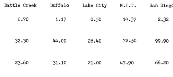
Table 4-1 shows the optimum system size, the

tax-exempt return on investment (ROI), and the taxable ROI for each of the sites. Note that the optimum system size was just above the lowest average monthly electric power

requirement for the M.I.T. site and the Buffalo site, while the optimum system sizes for the San Diego, the Battle Creek, and the Lake City sites were just at the

lowest average electric power requirement. This can be seen in Figures 4-1 through 4-5. This is an important

result because the optimum system size predicted without

any buy-back rate was that size just able to meet the

lowest average monthly electrical requirement (Flint,

1983). Therefore, the addition of utility buy-back rates had either a small or a negligible effect on the optimum

system size, depending on the site. It was further

determined that for those sites which did exhibit a larger

optimum system size with the addition of utility buy-back,

complete elimination of the buy-back rate only reduced the ROI by at most 7.5 percent of its original value. The

Battle Creek Buffein Lake City MoT LT, oan Diego OPTIMUM SYSTEM SIZE (MW) 1 9 nor 1h. n S

TAX-EXEMPT

Table 4-1 : Optimum Plant Size and Return on Investment Results

Lule

De70 Led? Ue 0 ho Le32

e730 «4,00 28.40 02-50 99.90

Wage =: - 15 - ..

5 — . — mo ee er st rt set rt eee ees eet ey eit hot hp WE

X System thermal output level

B10

O

TTT TTT me me - wo. a fem me = I

System electric output level

- od \ I

JUL AUG SEP oc NOV DEC JAN FEB MAR APR MAY JUN Month

Figure 4-1 : Cogeneration System Energy Output for San Diego Hospital

20

Laate

Sy

PTT TT TTTTTST

~ 8 - :

: _

7 Wag Waste

: _

: ro free a ww mt WS EE | Se Sed de eh een eens ot vy oi py To :

|

System thermal output level

System electric output level

| | I i

JUL AUG SEP OCT NOV DEC JAN FEB MAR APR MAY JUN Month

Figure 4-2 : Cogeneration System Energy Output for Battle Creek Hospital

12

,

z L I< id

’ System thermal ‘output level =

F System electrical output level

JUL AUG SEP OCT NOV DEC JAN FEB MAR APR MAY JUN Month

RG EE TTT

18

-37 os

5 10 rm

t Was:

8 | System thermal output level _

Eo. o_o

System electrical output level

-_ ) o-_o -_ ee

—--_ ~ oo -— —- Le —

: Utility buy-back

e—_ tt rrov_!Loa

JUL AUG SE; OCT NOV DEC JAN FEB MAL APR MAY JUN Month

Figure 4-4 : Cogeneration System Energy Output for Buffalo Hospital

0

FN

-»y

125 +

120 —

10°

90

=

-3 Was. System thermal output level

: 60 =e ______ =

l.

Lo

System electrical output level

t

" = TF - Tm eT = - TTT T= }

Utility buy-.

—_— C1

JUL AUG SEP OCT NOV DEC JAN FEB MAR APR MAY JUN Month

Figure 4-5 : Cogeneration System Energy Output for M.I.T.

rack

li

reason for this relative insensivity to reasonable buy-back rates is that the buy-back rate was not

sufficiently greater than the cogenerated electricity cost to justify the large additional capital expenditures

needed to bring the optimum system size appreciably above the lowest average monthly requirements.

Another important result of this portion of the analysis was that the optimum operating capacity never fell below the rated operating capacity. even though this

meant excess thermal production at times which just went

to waste. This suggests a strong fuel savings sensitivity to turbine efficiency.

Also note that San Diego and M.I.T. had substantially

higher ROIs than the other sites. This was a result of

the high electricity prices in these regions. A high

electricity price means more fuel savings due to the

cogeneration investment, and therefore a higher return on investment.

Figure 4-6 shows the optimal turbine size versus the

NPV to initial capital outlay ratio (as discussed in

section 3.2.2) for a typical site. It is clear that the

turbine which yielded the highest ROI fell within the

ob

Discount rate = 0.10) ]

pb VV

L 4 6 10 12 1 15¢I22c242.

System Size, MW

.F

LA

2 omy

4.2 Sensitivity analysis

4.2.1 Optimum system size

In general, 1t was found that the optimum system size was most sensitive to the buy-back rate, and the utility

electricity cost. The optimum size was found to be

sensitive to utility electricity prices only when the

buyback rates were high (M.I.T. and San Diego, and

Buffalo, see Figures 4-7 through 4-11). The optimum plant size increased with dropping electricity prices because substantial fuel savings could only be realized in this

situation if the cogenerator produced much excess

electricity to take advantage of the high buy-back rates.

Typically, the optimum system size increased substantially

with increasing buy-back rates for those sites which had

an initial increase in optimum size due to buy-back rates

(Figures 4-7 through 4-11). The size increased here

because the cogeneration systems produced electricity at

costs substantially lower than the high buy-back rates. The optimum turbine size increased to take advantage of the additional fuel savings until diminishing returns to

scale of the turbine were realized. Every other input

parameter had a negligible effect on the optimum system

c i ew

B — © 4

DQ 2.0 - .

N

wi. A. Electricity cost

E

5 1.0

% Change in Variable

Figure 4-7 : Turbine Size Sensitivity for

can Diego Hospital

T LE -_— __-B T.8 i

1h

Ee

A AL

_ —— 1|

% Change in Variable

Figure 4-8 : Turbine Size Sensitivity for

buffalo Hospital

-KB oC

x r

p :

or

5 2

Figure 4-9 : Turbine Size Sensitivity for

Lake City Hospital

50 "Wo (1 ah Ee ol A + a.

| KE

TA,B 3

Fo

E

Boo

% Change in Variable

Figure 4-10: Turbine Size Sensitivity for Battle Creek Hospital

2 22 2N

-a 18

bo16 |

z

& w |B Ay

wo Ley

-50 ln -20 0 20 LO AD

% Change in Variable

Figure 4-11: Turbine Size Sensitivity for M.I.T. J

Zé

2h

£2

4.2.2 Return on investment

Fiqures 4-12 through 4-16 show the sensitivity of the ROI to the economic and hardware input parameters. The

results here were fairly consistent with the ROI being

most sensitive to the utility electricity prices, somewhat less sensitive to natural gas costs and in two cases

(M.I.T. and Buffalo) to positive changes in the buy-back

rate, and minimally sensitive to such other parameters as

equipment lifetime, the standby charge, the inflation

rate, and the interconnection costs. Note that the ROI was

most sensitive to those parameters which directly determined the fuel savings.

Figures 4-17 through 4-21 show the sensitivity of the ROI to the tax and financing variables. With the exception

of utility electricity prices, the ROI is about as

sensitive to these variables as to the hardware and

economic variables. The ROI is most sensitive to the tax

rate and the percent of capital borrowed, and least

sensitive to the loan interest rate, the investment tax

credit, and the loan repayment period. This analysis

clearly shows that borrowing as much as possible against the capital cost is an advantageous strategy.

100 3u At dy 2

-50

Cb ’,6

2 IS

Y

=

3. Standby charge

-100 I i

Figure 4-12 : ROI Sensitivity to Hardware and

S54

7

v5

2

-3, Standby charge

4, Buy-back rate

5. System life

Figure 4-13 : ROI Sensitivity to Hardware and Economic

100 80

50

nT ——eSs=_—7—

a

& 1. Electricity price

o 2+. Gas price

No -ho 3. Standby charge

L, Buy-back rate 5. System life 6. Interconnection cost a 7. Inflation .. 4% -ln -20 0 20 Lo 60

% Change in Variable

Figure 4-14 : ROI Sensitivity to Hardware and Eco-nomic Variables for San Diego Hospital

56

ot ~L40 - 1, Electricity price

3. Standby charge

Figure 4-7" - ROI Sensitivity to Hardware and

Eco-nomic Variables for Battle Creek

Ir. J La Iu TAN ly J Tt 1 ot [ny Fi i ny -20 LL.

o

Cooks Em Ee Tw

- -20

@

= 1. Electricity price

50 7. Inflation

-an

% Change in Variable

Figure 4-16 : ROI Sensitivity to Hardware and Eco-nomic Variables for M.I.T.

50 >

Ln

-~D

x

-20 |

20 B. Percent capital borrowed

Ce Loan interest rate D. Investment tax credit

B. Loan repayment period

hn =

"7 ) | ,

~6n -t *Y 20 ” 0) 0 “0

% Change in Variable

Figure 4-17 : ROI Sensitivity to Tax and Financing

Hy 4 2U 1 ~\ el 7 T -Iv — B 3 ~~ an > 10 -— bn a — D % 0 oo — i D ’

-5-10 J od

B. Percent capital borrowed

. Ce Loan interest rate

D. Investment tax credit

BE. Loan repayment period

Ly ~

-AN =L =-20 0 “9 Lo 60

% Change in Variable

Figure 4-18 : ROI Sensitivity to Tax and Financing Variables for Lake City Hospital

60

D.B

@

B. Percent capital borrowed C. Loan interest rate

D. Investment tax credit

E. Loan repayment period

hn

-50 bee _

-60 =n -20 0 29 Lo 60

% Change in Variable

Figure 4-19 : ROI Sensitivity to Tax and Financing

50

C w— . I,

A 10 p E

&

B. Percent capital borrowed

C. Loan interest rate D. Investment tax credit

E. Loan repayment period

he

-50 ; St So ar

-An -hn on n 20 "1 A)

% Change in Variable

Figure 4-20 : ROI Sensitivity to Tax and Financing Variables for Battle Creek Hospital

62

50

Ju

A 10 —p :

B. Percent capital borrowed

Ce Loan interest rate D. Investment tax credit

E. Loan repayment period

“bn i}

re I i I

~~— _—— n

i -20 2 20 9 “9

% Change in Variable

Figure 4-21 : ROI Sensitivity to Tax and Financing

CHAPTER FIVE

CONCLUSIONS AND RECOMMENDATIONS

35.1 Conclusions

Comparing the optimum turbine sizes developed in this study to the optimum sizes expected without considering buyback rates, it was apparent that buy-back rates did not

have a pronounced effect on the optimum cogeneration

system size until the buy-back rates reached

unrealistically high values compared to the price of

electricity. It was also shown that even those sites which

did show an increase in the optimum turbine size due to buy-back rates had ROI’s which were relatively insensitive

to negative changes in the buy-back rates.

Potential cogeneration investors should be less concerned about uncertainties concerning those variables to which the ROI is insensitive, such as the buy-back rate, the inflation rate, the interest rate, or the

lifetime of the system, and much more concerned about

uncertainties in the electricity prices or in the marginal tax rate. Hopefully this report can help potential

investors decide which parameters are important in the

bl

and which parameters are less important to the decision and therefore deserve less consideration.

In an absolute sense, the returns on investment established in this report were quite high, and make the cogeneration investment look extremely attractive. In

addition to saving money, the potential cogenerators would be saving the country’s valuable and limited energy

resources.

2.2 Recommendations

This study should be augmented by taking into account the daily and hourly changes in thermal and electrical

loads at the potential cogeneration sites. The addition of

this parameter would probably reduce the calculated ROIs

of this report, and perhaps give a more realistic

assessment of the economic benefits of rather small scale

cogeneration systems such as those studied here. However,

the results of this study are promising. In cogeneration 1s a means of reducing the aggregate fuel consumption of the United States while reducing the energy financial burden of her citizens. 1 therefore recommend further

Federal policy incentives towards the future growth of

APPENDIX A

The following FORTRAN program was used to calculate the optimum

system size, the optimum turbine output for each month, and the

corresponding return on investment for the potential cogeneration

sites considered in this study. The energy consumption requirements

are read from a data file, while the user must enter the hardware,

66

& WRITTEN BY KEVIN A. MAYER, OCTOBER 1983, FOR UNDERGRADUATE MECHANI-CAL ENGINEERING THESIS. THIS INTERACTIVE PROGRAM OPTIMIZES GAS TURBINE

COGENERATION PLANT SIZE AND OPERATING CONDITIONS GIVEN ECONOMIC, ENVIRONMENTAL, AND TURBINE EFFICIENCY PARAMETERS. THIS PROGRAM

| ALSO GIVES THE OPTIMUM INTERNAL RATE OF RETURN THAT CAN BE EXPECTED

FROM THE INITIAL CAPITAL INVESTMENT IN THE COGENERATION SYSTEM.

: CHARACTER DECLARATIONS

INTEGER ZINC, YINC, YRS

PARAMETER (ZINC=10, YINC=20, GENEFF=.96, GBEFF=.98) LOGICAL TFLAG

REAL A, B, BBRATE, DR, EITC, GR, GRCOST, GASCOS, BOIEFF, INCCAP REAL INICAP, IRATE, ITC, INTCOS, LYRS, MAXCAP, LARGE, PRINC

REAL ROI, RPV, RSUM, SMALL, STBYCH, TAXRAT, AEFC(YINC), ALP (25) REAL ASFC (YINC), ADJBAS (0:ZINC), CAP (0:ZINC), CAPCOS (0:ZINC) REAL COST (YINC), DEP (25), ECOEFF (0:ZINC), ECOST (12), EDIFF (YINC)

REAL EEPCAP (YINC), ELOUT(YINC), ELREQ (12), FMMBTU(YINC), FSMAX (12) REAL FUEL (YINC), FUESAV (YINC), HEREQ(12), KOUT(0:ZINC,12)

REAL KSOUT (0:ZINC,12), LIP (25), MAXSAV(0:ZINC), MCAP (12), MOUT (12)

REAL NETSAV (0:ZINC,0:25), NPV(0:ZINC), PCAP(YINC), PV (0:ZINC, 25) REAL ONPV (0:ZINC), RR(1000), SCOST (12), STEFF (YINC), SDIEF (YINC) REAL STOUT (YINC), SOUT(12), SUM(O:ZINC), TEPCAP (YINC)

REAL TOTCOS (YINC), X(O:ZINC)

z READ IN NECESSARY DATA FROM TERMINAL AND DATA FILE DO 1 L=1,12

READ (5, *) ELREQ(L) ,HEREQ (L)

TYPE*, "MONTHLY ENERGY REQUIREMENTS HAVE BEEN ENTERED’

TYPE*, 'ENTER THE COST OF ELECTRICITY FROM UTILITY

TYPE*, 'IN CENTS PER KW-HOUR'

ACCEPT*,GRCOST

TYPE*, 'ENTER THE UTILITY BUYBACK RATE IN CENTS PER KW-HOUR'

ACCEPT*, BBRATE

TYPE*, 'ENTER THE COST OF GAS IN $ PER MILLION-BTU' ACCEPT* ,GASCOS

TYPE*, 'ENTER THE EXPECTED GROWTH RATE OF ENERGY’ TYPE*, 'COSTS AS A DECIMAL QUANTITY (5%=0.05)' ACCEPT*,GR

TYPE*, 'ENTER THE DESIRED DISCOUNT RATE FOR THE OPTIMIZATION’

TYPE*, 'PROCEDURE AS A DECIMAL QUANTITY ACCEPT*,DR

TYPE*, 'ENTER THE BOILER EFFICIENCY AS A DECIMAL QUANTITY’

ACCEPT* , BOIEFF

TYPE*, 'ENTER THE SLOPE OF THE GAS TURBINE EFFICIENCY CURVE'

ACCEPT*,B

TYPE*, 'ENTER THE INTERCEPT OF THE TURBINE EFFICIENCY CURVE IN KW'

ACCEPT*,A

TYPE*, 'ENTER THE INVESTMENT TAX CREDIT AS A DECIMAL QUANTITY ACCEPT*, ITC

TYPE*, 'ENTER THE ENERGY TAX CREDIT AS A DECIMAL QUANTITY' ACCEPT* ,EITC

TYPE*, 'ENTER THE INTERCONNECTION COSTS IN $ PER KW' ACCEPT*, INTCOS

TYPE*, 'ENTER THE STANDBY CAPACITY CHARGE IN $ PER KW PER MONTH'

ACCEPT*,STBYCH

3

ACCEPT*, YRS

TYPE*, 'ENTER THE FRACTION OF THE CAPITAL COST TO BE FINANCED’ TYPE*, 'AS A DECIMAL QUANTITY

ACCEPT* ,PRINC

TYPE*, 'ENTER THE LOAN INTEREST RATE AS A DECIMAL QUANTITY’

ACCEPT* , IRATE

TYPE*, 'ENTER THE EXPECTED TAX RATE AS A DECIMAL QUANTITY ACCEPT*, TAXRAT

TYPE*, ‘ENTER THE EXPECTED LOAN PAYBACK PERIOD IN YEARS' TYPE*, 'AS A REAL NUMBER (E.G. 18 YEARS= 18.0)’

ACCEPT*,LYRS

0 FIND LOWEST AVERAGE ELECTRICAL LOAD IN MW

>

SMALL=ELREQ (1)

IF (ELREQ (J) .LT.SMALL) SMALL=ELREQ (J)

. CONTINUE

XSMALL=SMALL/24./30.

INICAP=XSMALL/2.

INCCAP= (MAXCAP-INICAP) /REAL (ZINC) r

c INITIALIZE DEPRECIATION COEFFICIENTS TO ACRS 5 YEAR

pe DEP (1)=0.15 DEP (2) =0.22 DEP (3)=0.21 DEP (4)=0.21 DEP (5)=0.21 DO 10 N=6,YRS DEP (N)=0.0 1° CONTINUE

on USE DO-LOOP TO CYCLE THE CAPACITY FROM INICAP TO MAXCAP IN z ZINC INCREMENTS. INITIALIZE.

KFLAG=0 LARGE=0.0 TFLAG=.FALSE. DO 15 K=0,ZINC

CAP (K) =INICAP+REAL (K) * INCCAP

ECOEFF (K)=1.171/(1.+EXP (1.3964-0.14479*ALOG (CAP (XK) )))

DO 20 N=1,12 MELAG=1 FSMAX (N)=0.0

- FOR EACH MONTH, RUN THROUGH YINC DIFFERENT OPERATING

3 PERCENTAGES TO FIND OPTIMUM

DO 25 M=1,YINC

PCAP (M) =REAL (M) /REAL (YINC)

ELOUT (M) =PCAP (M) *CAP (K) *1000.

EEPCAP (M)=(1./B)- (1.-B*ECOEFF (K) ) * (A+B*CAP (K) *1000.) /B/

(A+B*ELOUT (M) )

TEPCAP (M) =EEPCAP (M) /GBEFF /GENEFF

68

FMMBTU (M) =FUEL (M) *0.003412

STEFF (M) = (1.-TEPCAP (M) ) *BOIEFF*0.97 STOUT (M) =STEFF (M) *FMMBTU (M)

SDIFF (M) =STOUT (M) -HEREQ (N) IF (SDIFF (M) .LT.0.) THEN

ASFC (M) =-GASCOS * SDIFF (M) /BOIEFF ELSE

ASFC (M)=0. ENDIF

EDIFF (M) =ELOUT (M) *24.*30.-ELREQ (N) *1000. IF (EDIFF (M) .GT.0) THEN

AEFC (M) =—EDIFF (M) *BBRATE /100. ELSE

AEFC (M) =—EDIFF (M) *GRCOST/100. ENDIF

COST (M) =FMMBTU (M) *GASCOS+ASFC (M) +AEFC (M) TOTCOS (M) =COST (M) +STBYCH*ELOUT (M)

TOTCOS (M) IS THE COST OF TOTAL ENERGY REQ'S FOR MONTH N WITH COGENERATION EQUIPMENT OF CAPACITY CAP (K) OPERATING

= AT CAPACITY PCAP (M)*CAP (K) . NOW FIND FUEL SAVINGS OVER

CONVENTIONAL SOURCES.

ECOST (N) =ELREQ (N) *1000. *GRCOST/100.

SCOST (N) =HEREQ (N) *GASCOS/BOIEFF

FUESAV (M) =ECOST (N) +SCOST (N) —“TOTCOS (M) z FIND M WHICH YIELDS MAXIMUM SAVINGS FOR MONTH N

IF (FUESAV (M) .GT.FSMAX (N)) THEN FSMAX (N) =FUESAV (M)

MFLAG=M ENDIF 27 CONTINUE

SOUT (N) =STOUT (ME LAG)

MOUT (N) =ELOUT (MELAG) 20 CONTINUE

MAXSAV (K) =FSMAX (1) +FSMAX (2) +FSMAX (3) +FSMAX (4) +FSMAX (5) +

1 FSMAX (6) +ESMAX (7) +FSMAX (8) +FSMAX (9) +FSMAX (10) +FSMAX (11) + : FSMAX (12)

DO 30 I=1,12

KSOUT (K, I) =SOUT (I)

KOUT (K, I) =MOUT (I) *24.*30./1000. a2 CONTINUE

CAPCOS (K) = (1660 .-120 . *ALOG (CAP (K) *1000.) ) *CAP (K) *1000. .

= USE NPV ANALYSIS TO CHOOSE OPTIMUM SYSTEM SIZE ADJBAS (K) =CAPCOS (K) * (1.-0.5% (ITC+EITC))

X (K) =PRINC*CAPCOS (K)

NETSAV (K, 0) =—CAPCOS (K) -~INTCOS *CAP (K) *1000. +X (K) +

(ITC+EITC) *CAPCOS (K) SUM (K) =NETSAV (K, 0) DO 35 I=1,YRS IF (I.GT.INT(LYRS)) THEN ALP (I)=0.0 LIP (I)=0.0 ELSE

ALP (I)=(l./LYRS + (1.-(REAL(I)-1.)/LYRS)*IRATE) *X (K)

35

15

60

ENDIF

NETSAV (K, I) = (1.~TAXRAT) * (1.+GR) **I* (MAXSAV (K)

-0.1*CAPCOS (K) ) +*TAXRAT* (DEP (I) *ADJBAS (K) +LIP (I) )-ALP (I) PV (K,I)=NETSAV(K,I)/(1.+DR)**I SUM (K) =SUM (K) +PV (K, I) 3 CONTINUE NPV (K) =SUM (K)

ONPV (K) =-NPV (K) /NETSAV (K, 0)

C FIND K WHICH GIVES LARGEST QNPV TO GET MAXIMUM IRR C

IF (ONPV (K) .GT.LARGE) THEN

LARGE=QNPV (K)

TYPE*, ‘NPV AT DISCOUNT RATE',DR, 'IS NEGATIVE' TYPE*, 'PLEASE ENTER A REDUCED RATE FOR EFFECTIVE'

TYPE*, 'OPTIMIZATION. PROGRAM TERMINATED. '

GOTO 999 ENDIF

C

C NOW FIND OPTIMAL INTERNAL RATE OF RETURN c RR (1)=0.001 ROI=RR (1) *100. DO 50 M=1,1000 RSUM=NETSAV (KELAG, 0) DO 60 N=1,YRS RPV=NETSAV (KFLAG,N) / (1.+RR (M) ) **N RSUM=RSUM+RPV : CONTINUE IF (RSUM.GT.0.) THEN RR (M+1)=0.001+M*0.001 ELSE ROI=RR (M) *100. GOTO 70 ENDIF IF (RR (M) .EQ.0.999) THEN

TYPE*, ' INTERNAL RATE OF RETURN EXCEEDS 99.9, ROI=99.9' ROI=99.9

GOTO 70 ENDIF 50 CONTINUE 70 CONTINUE

OUTPUT DATA AND CREATE OUTPUT FILE

DO 80 K=1,12

WRITE (6,101) K, ELREQ (K)

101 FORMAT (' THE ELECT. REQ. FOR MONTH',I3,' =',F12.2,' MW-H')

WRITE (6,102) K,HEREQ (K)

102 FORMAT (' THE HEAT REQ. FOR MONTH',I3,' =',F15.2,' MILL-BTU')

WRITE (6,103) K,KOUT (KELAG,K)

103 FORMAT (' THE ELECT. OUTPUT FOR MONTH',I3,' =',F12.2,' MW-H')

WRITE (6,104) K,KSOUT (KFLAG,K)

104 FORMAT (' THE HEAT OUTPUT FOR MONTH',I3,' =',F12.2,' MILL-BTU')

70

hy

WRITE (6, 200)

200 FORMAT (///)

WRITE (6, 105) CAP (KELAG)

105 FORMAT (' THE OPTIMUM SIZE OF PLANT =',F18.2. MW")

WRITE (6,106) ROI

106 FORMAT (* THE OPTIMAL RETURN ON INVESTMENT =',F9.2, %') WRITE (6.107) YRS

107 FORMAT (* THE LIFE OF THE EQUIPMENT =',I16,' YEARS')

WRITE (6,108) CAPCOS (KFLAG)

108 FORMAT (' THE CAPITAL COST OF THE EQUIPT. — .F9.0.' 8')

WRITE (6,109) PRINC

109 FORMAT (' THE FRACTION OF LOAN =',F21.2) WRITE (6,110) IRATE

110 FORMAT (' THE LOAN INTEREST RATE =',F19.2 “7

WRITE (6,111) NETSAV (KFLAG,0)

111 FORMAT (' THE CAPITAL OUTLAY IN YEAR O =',F13.2.' $') WRITE (6,112) LYRS

112 FORMAT (* THE LOAN REPAYMENT PERIOD =',F16.0," YEARS’) WRITE (6,113) TAXRAT

113 FORMAT (* THE TAX RATE =',F29.2,' %') WRITE (6,114) GRCOST

114 FORMAT (* THE GRID ELECTRICITY COST =',F16.2,' ¢/KW-H') WRITE (6,115) BBRATE

115 FORMAT (' THE BUY-BACK RATE =',F24.2,' $/KW-H') WRITE (6.116) GASCOS

116 FORMAT (' THE GAS COST =',F29.2,' $/MILLION-BTU') WRITE (6,117) INTCOS

117 FORMAT (* THE INTERCONNECTION COST =',F19.2,' $/KW') 999 STOP

APPENDIX B

The following is a sample output from the program in Appendix A.

The output reiterates the site energy requirements and the input

parameters and shows the results of the analysis. Please note that

77

THE ELECT. REQ. FOR MONTH 1 = 909.00 MW-H THE HEAT REQ. FOR MONTH 1 = 7000.00 MILL-BTU

THE ELECT. OUTPUT FOR MONTH 1 — 842.50 MW-H

THE HEAT OUTPUT FOR MONTH 1 = 7057.95 MILL-BTU THE ELECT. REQ. FOR MONTH 2 = 821.00 MW-H THE HEAT REQ. FOR MONTH 2 = 6400.00 MILL-BTU THE ELECT. OUTPUT FOR MONTH 2 = 842.50 MW-H

THE HEAT OUTPUT FOR MONTH 2 = 7057.95 MILL-BTU

THE ELECT. REQ. FOR MONTH 3 = 850.00 MW-H THE HEAT REQ. FOR MONTH 3 = 7000.00 MILL-BTU

THE ELECT. OUTPUT FOR MONTH 2 = 842.50 MW-H THE HEAT OUTPUT FOR MONTH 3 -: 7057.95 MILL-BTU

THE ELECT. REQ. FOR MONTH 4 = 821.00 MW-H THE HEAT REQ. FOR MONTH 4 = 8000.00 MILL-BTU

THE ELECT. OUTPUT FOR MONTH 4 - 842.50 MW-H

THE HEAT OUTPUT FOR MONTH 4 = 7057.95 MILL-BTU THE ELECT. REQ. FOR MONTH 5 = 674.00 MW-H THE HEAT REQ. FOR MONTH 5 = 15000.00 MILL-BTU

THE ELECT. OUTPUT FOR MONTH 5 = 842.50 MW-H THE HEAT OUTPUT FOR MONTH 5 = 7057.95 MILL-BTU THE ELECT. REQ. FOR MONTH 6 = 674.00 MW-H

THE HEAT REQ. FOR MONTH 6 = 170006.00 MILL-BTU

THE ELECT. OUTPUT FOR MONTH 6 = 842.50 MwW-H THE HEAT OUTPUT FOR MONTH 6 = 7057.95 MILL-BTU

THE ELECT. REQ. FOR MONTH 7 = 821.00 MW-H THE HEAT REQ. FOR MONTH 7 = 18000.00 MILL-BTU

THE ELECT. OUTPUT FOR MONTH 7 = 842.50 MW-H THE HEAT OUTPUT FOR MONTH 7 = 7057.95 MILL-BTU THE ELECT. REQ. FOR MONTH 8 = 674.00 MW-H THE HEAT REQ. FOR MONTH 8 = 1S000.00 MILL-BTU THE ELECT. OUTPUT FOR MONTH 8 = 842.50 Mw-H THE HEAT OUTPUT FOR MONTH 8 = 7057.95 MILL-BTU

THE ELECT. REQ. FOR MONTH 9 = 674.00 MW-H THE HEAT REQ. FOR MONTH 9 = 19500.00 MILL-BTU

THE ELECT. OUTPUT FOR MONTH 9 = 842.50 MW-H THE HEAT OUTPUT FOR MONTH 9 = 7057.95 MILL-BTU

THE ELECT. REQ. FOR MONTH 10 = 850.00 MwW-H THE HEAT REQ. FOR MONTH 10 = 16500.00 MILL-BTU

THE ELECT. OUTPUT FOR MONTH 10 = 842.50 MW-H THE HEAT OUTPUT FOR MONTH 10 = 7057.95 MILL-BTU

THE ELECT. REQ. FOR MONTH 11 = 850.00 MW-H THE HEAT REQ. FOR MONTH 11 = 10200.00 MILL-BTU

THE ELECT. OUTPUT FOR MONTH 11 = 842.50 MW-H

THE HEAT OUTPUT FOR MONTH 11 = 7057.95 MILL-BTU THE ELECT. REQ. FOR MONTH 12 = 879.00 MW-H THE HEAT REQ. FOR MONTH 12 = 8000.00 MILL-BTU

TEE ELECT. OUTPUT FOR MONTH 12 = 842.50 MW-H TZ HEAT OUTPUT FOR MONTH 12 = 7057.95 MILL-BTU

THE OPTIMUM SIZE OF PLANT = 1.17 MW

THE OPTIMAL RETURN ON INVESTMENT = 31.10 ¥%

THE LIFE OF THE EQUIPMENT = 15 YEARS

THE CAPITAL COST OF THE EQUIPT. = 950404. §

THE FRACTION OF LOAN = 0.00 THE LOAN INTEREST RATE = 0.00 ¥%

THE CAPITAL OUTLAY IN YEAR O = 869405.31 §

THE TAX RATE = 0.46 9 THE GRID ELECTRICITY COST = 6.41 ¢ /KW-H THE BUY-BACK RATE = 6.00 ¢ /KW-H

THE GAS COST = 4.34 $/MILLION-BTU THE INTERCONNECTION COST = 12.00 $/KW

li

REFERENCES

American Gas Association. "An Energy Conservation and Economic Analysis of Gas-Fired Cogeneration Technologies in Commercial and Industrial

Applications," Arlington, VA: August 1981.

Dames and Moore. "An Assessment of Cogeneration Potential in the

Northeast Utilities Service Area: Phase I and Proposed Phase II,"

Submitted to Northeast Utilities, Hartford, CT: January 1981. Energy User News. Volume 8, Number 45, NY, NY: November 1983.

Flint, B.B., "Return on Investment Analysis of Cogeneration Systems,"

Bachelor Thesis, M.I.T.: May 1983,

Gill, H.S.,"Federal Incentives for Cogeneration," Engineering Bulletin

56: July 1981.

Goodwin, L.M.,"A Special Report: Cogeneration and the Federal Tax Laws After the Economic Recovery Tax Act of 1981," Cogeneration World, Volume 1, Number 2: March 1982.

Hess, R.W., Turner, J.J., Krase, W.H., Pei, R.Y.,"Factors Affecting

Industry's Decicision to Cogenerate," Rand, Santa Monica, CA. McCaughey, J.,"The Supreme Court Breathes New Life Into Cogenerators,"

The Energy Daily, Volume 11, Number 95, Washington, D.C.: May 1983.

Office of Technology Assessment,"Industrial and Commercial Cogeneration,’

Washington, D.C.: February, 1983.

Pickel, F.H.,"Cogeneration and Utility Planning," PhD Thesis, MIT:

June 1982.

Shupe, D.S., What Every Engineer Should Know About Economic Decision

Analysis, NY,NY: Marcel Dekker, Inc.: 1980.

Standard Federal Tax Reports, "1983 Depreciation Guide," Commercial

Clearing House, Inc., Chicago, IL: May 1983.