A model to predict the variation in nutrient utilisation for different purposes (i.e., growth, gestation, milk and egg production) in monogastric animals

HAL Id: hal-02789455

https://hal.inrae.fr/hal-02789455

HAL is a multi-disciplinary open access archive for the deposit and dissemination of sci-entific research documents, whether they are pub-lished or not. The documents may come from teaching and research institutions in France or abroad, or from public or private research centers.

L’archive ouverte pluridisciplinaire HAL, est destinée au dépôt et à la diffusion de documents scientifiques de niveau recherche, publiés ou non, émanant des établissements d’enseignement et de recherche français ou étrangers, des laboratoires publics ou privés.

egg production) in monogastric animals

. Unew, . Inra, . Topigs Norsvin

To cite this version:

. Unew, . Inra, . Topigs Norsvin. A model to predict the variation in nutrient utilisation for different purposes (i.e., growth, gestation, milk and egg production) in monogastric animals. [Contract] D3.5, 2019. �hal-02789455�

FEED-A-GENE

Adapting the feed, the animal and the feeding techniques to

improve the efficiency and sustainability of monogastric livestock

production systems

Deliverable D3.5

A model to predict the variation in nutrient

utilisation for different purposes (i.e.,

growth, gestation, milk and egg production)

in monogastric animals

Due date of deliverable: M48

Actual submission date: M48

Start date of the project: March 1

_{, 2015}

_{Duration: 60 months}

Organisation name of lead contractor: UNEW

Revision: V1

Dissemination level

Public - PU X

Confidential, only for members of the consortium (including Commission Services) - CO

Table of contents

1.

Summary ... 3

2.

Introduction ... 4

3.

Method ... 6

4.

Case studies ... 7

4.1

Growth of live weight in boars ... 7

4.2

Egg production in hens ... 7

4.3

Gestation and lactation in sows ... 8

5.

Results ... 9

5.1

Growth of live weight in boars ... 9

5.2

Egg production in hens ... 11

5.3

Gestation and lactation in sows ... 14

6.

Discussion ... 16

7.

Conclusions ... 18

8.

Annexes ... 19

8.1

Annex 1: Diagnostics of model fitting and data outliers ... 19

8.2

Annex 2: Bibliographic references ... 21

1. Summary

Objectives

The purpose of the model is to quantify the variability in individual trait responses within a livestock population whose individuals share a common factor, e.g., are of the same breed, live in the same farm, or are offered the same feed. In addition to assessing trait variability within a given a population, the approach will also allow comparisons between populations, e.g., that differ in species, breed, environment, or feed, accounting for both their average and their inherent variability in trait responses. The Deliverable has the following objectives towards these aims:

1) To characterise and estimate trait variability from a dataset on a herd, flock or breed.

2) To predict and summarise the influence of variation in model-derived traits on trait variation in a production system.

3) To demonstrate the approach on different monogastric species and on performance and reproduction traits.

Rationale:

We developed a modelling approach that has multiple applications in precision livestock farming, nutrition, and selective breeding. The approach is demonstrated through three case studies on monogastric livestock: growth in pigs, and reproduction in sows and in laying hens. Comparison of trait variability across these species and traits shows common aspects that they share as well as their distinctive features. This methodology comprises a data-driven (top-down) approach, where models are fitted to phenotypic trait data obtained from multiple individual animals; and a simulation (bottom-up) approach, where population phenotypic variation is derived and summarised by the average and deviation (i.e., median and confidence interval) for each modelled trait. The approach has the following benefits in relation to current alternatives: 1) Making no prior assumptions about the distributions of traits and their correlations within the population; specifically, it is assumed that the population traits are distributed according to the trait distribution in the group of sampled animals (non-parametric approach). 2) Being computationally faster than current (non-parametric approaches; specifically, the distribution of traits in the wider population is inferred from that in the sample through a process of individual resampling. 3) Having no specific requirements on the size and quality of the datasets input.

Teams involved: UNEW, INRA, Topigs

2. Introduction

Motivation

It is necessary to introduce stochasticity (i.e., variation) in predictive models of livestock production to account for trait variation across individuals in a herd, flock or breed. The introduced stochasticity should preferably be based on empirical data, because different forms of modelling stochasticity in individual traits can lead to disparate conclusions about variation in populations.

There are important benefits from accounting for phenotypic variation in model predictions rather than using predictions solely for the ‘average’ animal (Kyriazakis, 2011; van Milgen et al., 2012; Saintilan et al., 2013; Filipe et al., 2018a; Pomar et al., 2018; Filipe and Kyriazakis, 2019; Tullo et al., 2019); these include the following:

1) Knowledge of the range and distribution of individual output within a group provides the user with information about deviations from the average individual output; moreover, it offers users a more accurate prediction of the group’s total output, i.e. the total is usually different from (average productivity) x (number of animals).

2) This knowledge also allows prediction of the level of uniformity in the group (e.g., how many individuals conform to market requirements) and thus allows prediction of the current market value of a given batch, herd or flock.

3) Knowledge of the dynamic performance of each individual or each pen, allows for real-time implementation of individually- or pen-targeted feeding and health-improvement schedules for optimal allocation of resources.

4) Prediction of the variation in model-derived traits within a population can assist the achievement of breeding goals when genetic selection utilises model-derived traits.

5) A more robust comparison between populations (e.g., different breeding lines) in different environmental conditions, or offered different diets.

These benefits will help breeders and producers, improve animal welfare, and reduce environmental impact by contributing to the implementation of modern precision livestock farming practices (PLF), and, therefore, will contribute to the broader aim of delivering greater sustainability and robustness in intensive livestock production systems.

Problem

Estimating and modelling variation in traits requires much more computation than estimating and modelling an average animal. In other words, instead of doing one calculation, we need to perform many calculations, which is has extra computational cost. The approach that we have developed and implemented here is a trade-off between this extra computational cost and the benefits from having information on the deviations from the average.

Progress has been made in animal science to predict the distribution of animal productivity within populations (Ferguson et al., 1997; Knap et al., 2003; Pomar et al., 2003; Vautier et al., 2013). This methodology relies on two steps. First, the assumption and calibration of a certain plausible distribution of model trait parameters in the population; typically, a multivariate-normal distribution of parameters calibrated via an empirical or expert-based variance-covariance matrix (top-down approach). Second, the simulation of the trait variation in the population under the assumed distribution (bottom-up approach). There are several disadvantages in assuming explicit population trait distributions, such potential inaccuracy and difficulty of calibration.

Approach taken

We develop a combination of top-down and bottom-up approaches that has two important features (Filipe et al, 2018a; Filipe and Kyriazakis, 2019). First, the methodology is non-parametric, i.e., it draws the trait distribution and correlations implicit in the empirical data without making explicit and potentially inaccurate assumptions about such distributions and correlations. Second, the methodology requires much less computation than using the latter assumptions, because it does not require the construction of and simulation from a hypothetical trait distribution. In the top-down step, a data-driven approach is applied where models are fitted to phenotypic trait data obtained from multiple individual animals. In the bottom-up step, the following approach is applied for estimating population phenotypic variation. Instead of assuming a theoretical distribution or expert-informed parameter ranges, it is assumed that the population traits are distributed according to the trait distribution in the group of sampled animals. This assumption is common to a broad range of non-parametric approaches. In addition, the distribution of traits in the wider population is inferred from that in the sample through a process of random individual resampling. The approach is completed by a statistical evaluation of the average and deviation (i.e., median and confidence interval) of each modelled trait in the population. Regarding the literature, this method contains assumptions that relate (but are not identical) to those made in bootstrap (Efron, 1982) and quantile regression (Koenker and Bassett, 1978) and combines them with other modelling components.

Scope

This modelling approach applies to the prediction and quantification of phenotypic variation within populations of different species, breeds, and herds of livestock. The phenotypic variation can comprise any number of traits that are measured or model-derived, and the correlations among traits are inherently preserved. The approach can be used for multiple purposes. Here, we focus on a selection of non-ruminant livestock species and performance and reproduction traits relevant to applications in farming, nutrition, and selective breeding.

3. Method

A first requirement in modelling population phenotypic-variation is the availability of longitudinal trait observations from multiple individual animals. These individuals are a sample from the relevant large population or are the full population. The first stage in the method (Filipe et al., 2018a; Filipe and Kyriazakis, 2019) is to estimate the stochasticity in trait parameters across the population (top-down approach); here, model curves are fitted to each individual dataset and their associated trait parameters are estimated. The second stage is to quantify the variability in the relevant traits that is a consequence of this stochasticity (bottom-up approach). The detailed components of the method are the following.

1-Assumption. The distribution of a given set of animal traits within the large

population is represented by the joint variation of these traits across the individuals in the sample taken from that population. As a result, the variation in other, model-derived traits will be naturally associated to the variation in observed traits among the individuals in the sample.

2-Variability in trait parameters. Trait parameters for each individual in the sample

are estimated by fitting a model to the observed traits. There are different techniques for fitting data and estimating parameters. Given that the models are non-linear, we used non-linear least-squares point estimation; other estimation techniques would also be suitable for this purpose (Filipe and Kyriazakis, 2019). The outcome is a distribution of model-based trait parameters across the sample. According to the assumption, this distribution is representative of that in the large population.

3-Resampling. The variation in model-derived traits in the large population is inferred

by resampling individuals randomly from the sample, repeatedly up to a chosen population size. This step has the effect of making the statistical value of the quantiles (evaluated below) converge to a stable value as the size of the resample becomes large compared to the size of the sample (unless the sample is very large, in which case both values should agree). As, according to the assumption, the individuals in the resample are repeated from the sample, no further computation of the model traits is required, only a recalculation of the statistics of these model traits. The resampling step is optional. The alternative is to use the sample itself, in which case the inferences do not extrapolate to a large population. The choice of whether to focus on trait distributions within the sample or in a larger population depends on the specific application and on the relevant question addressed (see applications in Discussion).

4-Quantiles of the trait distribution. For dynamic traits, a set of time points (or points

on another covariate) are chosen. The set can be within or, in the case of forecast or hind-cast, beyond the longitudinal range of the data. For each modelled trait, quantiles of its distribution (in the resample or sample) are evaluated at each time point. Here, the 5%, 50%, and 95% quantiles were used to represent the trait average (via the median) and confidence interval (area between the 5% and 95% quantile curves, which

contains 90% of the individuals in the population). Examples of dynamic traits are live weight and protein weight. Non-dynamic traits associated to the latter are the live weight and protein weight at a given stage (e.g., maturity), or the average weight gain or protein deposition over a given period. For non-dynamic traits, quantiles are evaluated only once. A modelled trait can be a model representation of an observed trait (e.g., live weight or live weight gain) or a model-derived trait that is not observed but is related to observed traits via biological assumptions (e.g., the intrinsic growth rate, dynamic or mature protein weight, or mature live weight) if not observed.

Diagnostics of model fitting and data outliers. The user of the method may wish to

check the quality of the model fitting or to identify and tackle potential outlier individuals in the population sample. A detailed account of the diagnostics on fitting and outliers and example diagnostic results (case study 1) is given in Annex 1.

4. Case studies

4.1

Growth of live weight in boars

 Data was provided by Topigs.

 Datasets: Individual data on live weight of boars of a single breed during the finishing growth: 119 animals; weight range 25-165 kg. The animals are a contemporary cohort offered the same dietary schedule ad libitum.

 Production model: Gompertz curve fitted to live weight (Filipe et al., 2018a). Other growth models could be used without altering the general outcomes of the method.

4.2

Egg production in hens

 Data was provided by INRA.

 Datasets: Individual data on hen egg laying and egg weight in two experimental lines divergently selected for residual food intake: 29 animals; age range while laying was 19-38 weeks; weighing of the eggs took place during 28-31 weeks of age. The lines are part of a long-term experimental programme (Bordas et al., 1992). The data from the two lines (one with 16, another with 13 animals) were merged into a single population sample to increase the sample size. While it is expected that reproduction traits are not significantly affected by this selection, some differences between lines are still likely. For our purpose of illustrating the approach, it is adequate to consider a genetically heterogeneous group, which tests the approach in the characterisation of potentially large phenotypic variation. Future applications of the approach could focus on the differences between these lines.  Production model: Gompertz curve fitted to egg output; power-law curve fitted to

4.3

Gestation and lactation in sows

Sow datasets at individual level and with longitudinal observations, as in the other case studies, were currently not available. As an alternative, we used simulated data, i.e. phenotypically-diverse outputs from a model where the variation is not informed by observation data. This case study allows us to demonstrate that: 1) gestation and lactation traits can be characterised using this approach in the same way that other traits can; and 2) the approach can be used for analysing artificial trait variability as well as trait variability based on observations. In addition, this case study shows that when it is advantageous to use simulated rather than observation-based population data, trait variability within the simulated population can still be adequately characterised.

Assumption: To simulate artificial phenotypic variability, trait parameters that are

inputs of the model were varied under the assumption that their range of variation is representative of the parameter distribution that would be obtained if the model were fitted to data from multiple individual sows. Such approach to generating phenotypic variability in a model population relates to those used in animal science (Knap et al., 2003; Pomar et al., 2003; Vautier et al., 2013).

 Data simulated by INRA.

 Datasets: Individual data on four sow traits during gestation and lactation: 26 simulated animals, during eight parities (first service at 140 kg and mature body weight after farrowing of 270 kg).

 Generation of data was via the model of Dourmad et al. (2008):

o Output traits: Live body weight, body protein, and body lipid during gestation and lactation; milk produced during lactation.

o Variability in input traits: These model output traits were simulated for each of

26 sows with distinct artificially-defined phenotypic profiles. This phenotypically-diverse population was constructed as follows. 1) A basic individual profile was defined by setting typical values of key sow and litter trait parameters in the model, such as sow body weight, backfat thickness, and feed intake at given critical stages of the production cycle, and piglet growth and survival. A facility of the model was used to ensure that the model output traits of the sow, such body weight and backfat thickness, did not deviate from the defining inputs throughout the long period of the simulation (eight parties, >1000 days); this involved calibrating the maintenance energy expenditure during gestation and lactation, and the minimum protein mobilisation during lactation. 2) Each of the other 25 individual sow profiles in the population was defined by changing one of the following traits: sow feed intake during lactation (basic value 5.8 kg/d, range 5.22 to 6.5 kg/d), sow body weight loss during lactation (basic value 25 kg, range 22 to 28 kg), and number of piglets born alive (basic value 12.5, range 10.5 to 14.5);

in each of these individuals no more than one trait was changed with respect to the basic sow profile because the trait correlations across sows are not known.

5. Results

5.1

Growth of live weight in boars

The live weight observations of the 119 boars (Figure 1A) show that each individual has a distinct growth trajectory and a specific age range during which weight was recorded. The X-axis ranges from the median first age of recording (76 d, 33 kg) to the maximum age of recording across animals (196 d, 167 kg); it does not start at the minimum first age of recording because there are too few individuals at the earlier ages of recording to estimate population quantiles.

The average (median) and confidence interval (CI, area between the 5% and 95% quantiles) characterise adequately the distribution of live weight across the population over the recorded finishing period (Figure 1B): approximately 10% of the individuals are outside the CI. The quantiles are based on resampling 1000 individuals out of the sample of 119 animals.

The median live weight has an inflection point around age 175 d (Figures 1C and E), which is very close to the average age of maximum growth for males of this breed (Egbert Knol, personal communication). An estimate of the inflection point based on the median is generally more robust and thus preferable to one based on the mean, because the median is not sensitive to outlier animals. The predicted daily gain, which is above 1 kg/d for only a short period (Figure 1E), is also in agreement with empirical expectation for this breed.

Prediction beyond the observed range shows the expected population average and CI up to 250 d (Figure 1D). The future width of the CI indicates how variability in weight might increase as the animals in the herd grow further. The CI width quantifies both predicted variability and uncertainty about future growth. The degree of uncertainty depends on the amount of information and noise in the past data; therefore, it is possible and plausible that a CI is wider than expected in practice, especially if the expectation were based on average observations (i.e., without deviations). Real-time prediction, where performance in the following day or period is predicted based on performance in a previously recorded period, could be tested by fitting the model to a narrower age range than in Figure 1D and predicting performance based on the parameters estimated using the narrower range. It is likely that the average would not be significantly affected, but that the CI would be wider than that based on the full data as in Figure 1D.

Diagnostics of model fitting and data outliers

The user of the method may verify the quality of the model fitting to the boar data or identify and tackle potential outlier animals in the sample. Results of the diagnostics on fitting and outliers are available (Figure 2 in Annex 1).

Figure 1. Growth in boars. A) Observed individual trajectories. B) Predicted population average (median) and 90% CI, overlapped on the data to which the model was fitted to individual by individual. C) As B, but without showing the dataset; note the average age at maximum growth (inflection point) at 175 d. D) Prediction as in B, but beyond the data range (197 d) to 250 d. E) Daily rate of weight gain, population average and CI; the maximum gain occurs at 175 d; an alternative evaluation of the average daily rate of weight gain (blue line, obtained by differentiating the average curve in B) is close but is a less suitable estimation.

5.2

Egg production in hens

Egg output

The observed number of eggs laid by each of the 29 hens (Figure 3A) shows that each individual follows a distinct production trajectory since the age of start of laying and during the given period of observation. The age of start of laying differed among hens (19-23 wk), but here we focused on the production trajectory of each hen regardless of the age of start of production.

The average and CI characterise suitably the distribution of egg output across the population over the recorded laying period, as approximately 10% of the individuals are outside the CI (Figure 3B). The CIs are determined by the fitted model trajectories (Figure 3C) and are based on a 1000-large resample. The noise in some extreme observed trajectories makes them differ somewhat from the fitted trajectories (Figure 3C), leading to some difference between outliers in Figures 3B and 3C. However, the average curve is robust to such variation.

The population average and CI of eggs output are prediction beyond the data range, up to 30 wk of laying (Figure 3D). In principle, it is possible to predict egg output up to any future point, and even to predict lifetime production individually and across the population. However, the shortness of the observed laying period (up to 18 wk) compared to the typical duration of laying (up to 2 years, depending on genotype), does not make for reliable long-term prediction; this is perhaps suggested by the shape of the average and CI beyond the data range.

The average daily rate of egg output declines consistently over time, although it is relatively constant up to 10 wk (Figure 3E). The decline at the end of the observations is probably excessive, which is likely a result of the short duration of the observations.

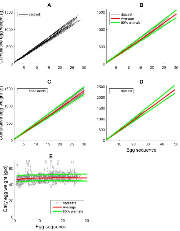
Egg mass

The cumulative egg mass produced during the laying sequence also shows variation among individuals, suggesting that some hens produce larger eggs (with the exception that a few hens lay multiple eggs on some days (Figure 3E), which does not imply larger eggs). A difference relative to egg output is that cumulative egg mass (along the egg sequence) is less variable within each individual’s production history. The predictions up to 30 wk in laying are similar to but reflect the lesser variability than in egg output (Figures 4A-D). The average daily egg mass produced increased slightly during laying, but the corresponding population variation is nearly constant, (i.e., egg weight variation occurs among and not within hens; Figure 4E) as already suggested by Figure 4A.

Figure 3. Cumulative egg output of each hen over time since start of laying. A) Observed individual trajectories; the age of start of laying varies among hens (19-23 wk) but is not included here in order to focus on the period of production. B) Predicted population average (median) and 90% CI, overlapped on the data to which the model was fitted to individual by individual. C) As B, but showing individual model-fitted trajectories. D) Prediction as in B, but beyond the data range (18 wk) to 30 wk laying. E) Daily rate of egg output, population average and CI; the rate of egg laying decreases slowly but consistently (as also evident from A-D).

Figure 4. Cumulative eggs mass laid during the laying sequence. Similar to Figure 3, but focusing on the mass of individual eggs (during 28-31 wk of age, i.e. 28 d) in terms of the ranking in laying sequence. A) Observed individual trajectories. B) Predicted population average (median) and 90% CI, overlapped on the data to which the model was fitted to individual by individual. C) As B, but showing individual model-fitted trajectories. D) Prediction as in B, but beyond the data range (29 eggs were laid) to 50 eggs laid. E) Daily egg mass laid, population average and CI; the egg mass increases very gently throughout. In the majority of occasions, the egg mass is that of a single egg laid; on a few occasions, some individuals laid >1 egg (i.e., 2 or 3; Figure 4E), in which cases the egg mass is that of the total eggs laid.

5.3

Gestation and lactation in sows

There is large variability in the four modelled traits of a gestating and lactating sow: live weight, protein weight, lipid weight, and mass of milk produced, both within the population and over time (i.e., across and within parities) (Figure 5A-B and E-F). The trait distributions, generated under the working assumptions (Case Study 3), are denser in the centre, which represent sows of similar phenotype expression (those that differed in body weight loss during lactation). Above and below the centre, the distributions are relatively evenly dispersed, representing sows of differing litter size or feed intake level. The distributions are not symmetric (Figure 5A or B), and there is no reason they should be. Milk production (Figure 5F) occurs only during the lactation. In the model used (Dourmad et al., 2008), milk production is not sensitive to some of the defining traits varied as a result of key assumptions on which the model builds.

Clearly, these artificial-trait distributions are suitable for illustrating how the method characterises variability in sow populations. The median of each trait (Figure 5C-D and G-H) tracks the time trend within in the sampled population. The medians also happen to be close to the centre of the distributions (Figure 5A-B and E-F) because the sow population was built to be relatively symmetric, but could deviate from the centre if the distributions were more asymmetric.

The CIs follow the temporal trend of the averages and characterise the variability within the population, e.g. only a few of the 26 individuals are outside the 90% CIs. These CIs show that there is considerable deviation from the average, but to a degree that depends on the trait. Such differences are more clearly seen by examining the deviations relative to the average (DRtA = (Y(t)-Yav(t))/Yav(t) where Y is the response and t is time) (Figure 6). Population deviations from the average are larger during lactation as the sow’s body resources are used to respond to the increased requirements of the piglets (which grow faster and are more physically active than during gestation). At its largest, the CI DRtA is 10% for live weight, <10% for body protein, and >20% for body lipid (Figure 6A-C).

Describing the population using the average curve would miss out important information: the amount of deviation from the average, how this deviation changes over time, and how the deviations differ among traits. On the other hand, describing such phenotypic characteristics would be difficult using serial observations across individuals (if such data were available) or multiple individually-fitted curves. That purpose is achieved adequately and simply by the CIs. The predicted CIs do not rely on assumptions about the population distribution and correlations of the traits and, therefore, are robust for applications to large numbers of simultaneous traits and to complex trait dynamics where the correlations may be unknown.

The relative deviations in protein and live weight within the population are comparable and appear plausible, while those for lipid weight are considerably larger. This fact results from the underlying assumptions of the sow model, where that all energy intake not used for protein deposition or maintenance is deposited as lipid (Dourmad et al., 2008). In practical applications, the levels of maintenance energy and protein mobilisation during lactation are adjusted so that lipid and body mass remain stable across the multiple parities. This adjustment was not implemented here, which explains the variation in lipid. These technical aspects illustrate practical difficulties in modelling sows over multiple parities, but are not relevant to our purpose of illustrating the potential of the approach to characterise phenotypic variation in general. Moreover, while we could have focused on a single parity, we preferred to show the potential of the approach to capture population variation with complex changes over time.

Figure 5. Gestation and lactation in sows. A-B, E-F) Artificial dataset of individual-sow trajectories for each of the traits considered: live weight, protein weight, lipid weight, and mass

Figure 6. Gestation and lactation in sows. Deviation of the 90% CI with respect to the population average (DRtA). A, B, C, D correspond to C, D, G, H in Figure 2. Other details as in Figure 5.

6. Discussion

The modelling approach developed here quantifies and predicts variation in animal traits within populations using empirical data from livestock herds or flocks. The results demonstrated the approach on growth and reproduction traits in monogastric livestock, i.e. growing pigs, and reproducing sows and laying hens. Comparison of trait variability across the species and traits considered showed common aspects that they share, e.g. growth in pigs and egg output in hens, as well as their distinctive features, e.g. egg output and egg mass in hens and gestation and lactation in sows.

Approach benefits

The approach makes no prior assumptions about the distributions of traits and their correlations within the population (Filipe et al., 2018a; Filipe and Kyriazakis, 2019). Additionally, the approach is computationally faster than parametric approaches by relying solely on model computations for the observed individuals, and thus avoiding model and statistical computations pertaining to hypothetical individuals drawn from an assumed trait distribution. Moreover, the approach has no specific requirements on the size and quality of the datasets input.

Data characteristics

The traits whose variation is predicted can be traits that are observed, i.e. at points during growth, or that are not observed such as model-derived traits, e.g. body lipid and protein in the sow example. The approach works both for empirical samples that have a small or a large number of individuals, and regardless of whether the longitudinal observations are smooth or noisy. In addition, the approach can quantify variation in datasets not from empirical samples but from model output generated under plausible assumptions, e.g. ranges or distributions of trait parameters, as in the sow case study.

Application areas

The approach can be used for multiple purposes in precision livestock farming, nutrition, and selective breeding. For example, if the animals in the dataset have been offered identical feed, the estimated variation can be attributed to genetic and environmental influences. Conversely, if the animals have been offered different diets or feeding schedules, the estimated variation includes the influence of nutrition. Moreover, if two or more datasets are considered from groups with distinct diets but similar variation in genetics and environment, then differences in the influence of these diets can be assessed and tested in a way similar to regression analysis but without the associated parametric assumptions. The same holds for comparisons among groups that are genetically distinct.

Such information about variability can help, for example, to quantify trait heritability, to implement targeted feeding and preventive treatments, or to make more realistic evaluations of livestock value, losses, and costs. For example, this approach was used to evaluate the economic gains from adopting alternative strategies for pig allocation to finishing pens (Filipe et al., 2018b). Applications can also be made to real-time prediction: given a trait observed over a window of time, its future average and population confidence interval can be predicted based on the earlier observations. For example, the prediction of the next-week’s intake and performance of a group can be carried out in this way.

While the results focused on specific species and traits, this modelling approach applies to any livestock species and genetic line and to any set of traits for which individual observations are available across a group. Therefore, on one hand, the approach allows the identification of commonalities and differences across species and lines. On the other hand, the approach allows consideration of other types of traits that affect production. For example, the degree to which production efficiency and robustness under disturbance are mutually exclusive or not, can be quantified by examining the joint variation and overlap of these traits in the same way that simultaneous traits of sows and hens were examined here.

7. Conclusions

A modelling approach was developed to quantify the phenotypic variation in animal traits within populations using empirical data from livestock herds or flocks, as well as to predict traits and their variation outside the range of empirical observation. The approach can also be used to quantify and predict trait variation in artificial data from simulation models. The approach has generic applications, including precision livestock farming, nutrition, and selective breeding in animal populations. First, the approach applies to any animal traits, although it was demonstrated here for growth and reproduction traits. Second, the approach applies to observable traits as well as to non-observable traits that can be related to the observed traits through a quantitative model. Third, the approach applies to monogastric livestock species as well as to any livestock species for which individual data are available. The advantages of the approach are its flexibility, i.e. no reliance on potentially-inaccurate assumptions about the form of variation and correlation of traits across individuals; its economy and speed of computation; and its applicability to small as well as to large animal sample sizes. Given the broad range of potential uses of this approach in the implementation of precision livestock farming, and the resulting benefits of precision livestock farming for producers, for animal welfare and for the environment, the approach has the potential to contribute to the broader aim of delivering greater sustainability and robustness in intensive livestock production.

8. Annexes

8.1

Annex 1: Diagnostics of model fitting and data outliers

The predictions of trait variability in a population (Figure 1) are the ultimate purpose of the current analysis; in general, no further results need to be examined. However, the user of the method may wish to verify the quality of the model fitting or to identify and tackle potential outlier individuals in the population.

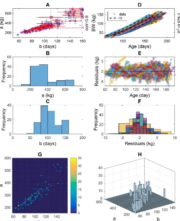
 Parameter distribution. The outcomes of fitting a Gompertz curve to the live weight of each individual (Figure 1A) are point estimates of the two parameters of this growth model (i.e., mature size and growth rate). The population distribution of these model-derived traits and the respective confidence intervals can be examined, either as a joint distribution or as separate marginal distributions (Figure A2.A-C).

 Goodness-of-fit. Goodness-of-fit was quantified by the coefficient of determination R2 _{and distribution of residuals (i.e., deviations of the data with respect to the model}

(Figure A1.E-F). The overall goodness-of-fit was high for most individuals, but a few individuals show a residual trend indicating that their specific growth conditions may have been disturbed and may not be describable by the proposed growth curve (Figure A1.D).

 Outliers. Some individual growth trajectories stand out with respect to the majority (Figure 1A), which could have been caused by a variety of factors, including disease. For these individuals, growth conditions may have been affected by extreme perturbations or observational errors, in which case the growth model and the fitting approach may no longer be appropriate. Consequently, the parameter estimates may not be compatible with their biological interpretation, and the resulting fitted curve may be an outlier in the population distribution model curves. We have used the option of tackling outliers by imposing presumed ‘acceptable’ bounds on the parameter ranges prior to their estimation; these ranges are reflected in the edges of Figure A1.A. Other approaches, such as the removal of identified outliers could be implemented.

 Resampling. The effect of resampling individuals from the original sample has the effect of increasing the relative counts and stabilising some of the quantile estimates (Figure A1.G-H).

Figure A1. Growth in boars – Diagnostics of model fitting and outliers. The outcomes of fitting the Gompertz curve, Y=a*(Y0/a)^{exp(-(X-X0)/b)), to each individual dataset (X,Y), where parameters (a,b) are the mature weight and time scale of growth (1/rate of growth), and vectors X and Y are the sequences of observed age and live weight: A) Population joint distribution of the point estimates of (a,b) and associated 95% confidence intervals. B-C) Marginal frequency distributions of parameters a and b. D) Fitted curved and datasets. E) Sequential residuals (deviations of the date from the model) for each individual. F) Frequency distribution of residuals for each individual. G-H) Population distribution of parameters in 1000 large random re-sample.

8.2

Annex 2: Bibliographic references

Bordas A., Tixierboichard M., Merat P. (1992). Direct and correlated responses to divergent selection for residual food-intake in rhode-island red laying hens. British Poultry Science 33 : 741-754.

Dourmad J.Y., Etienne M., Valancogne A., Dubois S., van Milgen J., Noblet J. (2008). InraPorc: A model and decision support tool for the nutrition of sows. Animal Feed Science and Technology 143: 372-386.

Efron B. (1982). The jackknife, the bootstrap and the other resampling plans, Philadelphia, PA., Society for industrial and Applied Mahtematics.

Ferguson N.S., Gous R.M., Emmans G.C. (1997). Predicting the effects of animal variation on growth and food intake in growing pigs using simulation modelling. Animal Science 64: 513-522.

Filipe J.A.N., Leinonen I., Kyriazakis I. 2018a. The quantitative principles of animal growth. In: Feed Evaluation Science (P.J. Moughan, W.H. Hendriks, eds.), pp. 387-422, Wageningen Academic Publishers, The Netherlands

Filipe J.A.N., Vogelzang R., Knol E., Kyriazakis I. (2018b). Pen-allocation strategies for uniform weights in finishing pigs. In: Feed-a-Gene 3rd _{Annual Meeting,}

Newcastle University.

Knap P.W., Roehe R., Kolstad K., Pomar C., Luiting P. (2003). Characterization of pig genotypes for growth modeling. Journal of Animal Science 81: E187-E195. Koenker R., Bassett G. (1978). Regression quantiles. Econometrica 46: 33-50.

Kyriazakis I. (2011). Opportunities to improve nutrient efficiency in pigs and poultry through breeding. Animal 5: 821-832.

Pomar C., Andretta I., Hauschild L. 2018. Meeting individual nutrient requirements to improve nutrient efficiency and the sustainability of growing pig production systems. In: Achieving sustainable production of pig meat (J. Wiseman, ed.). Burleigh Dodds Science Publishing.

Pomar C., Kyriazakis I., Emmans G.C., Knap P.W. (2003). Modeling stochasticity: Dealing with populations rather than individual pigs. Journal of Animal Science 81: E178-E186.

Saintilan R., Mérour I., Brossard L., Tribout T., Dourmad J.Y., Sellier P., Bidanel J., van Milgen J., Gilbert H. (2013). Genetics of residual feed intake in growing pigs: Relationships with production traits, and nitrogen and phosphorus excretion traits. Journal of Animal Science 91: 2542-2554.

Tullo E., Finzi A., Guarino M. (2019). Review: Environmental impact of livestock farming and Precision Livestock Farming as a mitigation strategy. Science of the Total Environment 650: 2751-2760.

van Milgen J., Noblet J., Dourmad J.Y., Labussiere E., Garcia-Launay F., Brossard L. (2012). Precision pork production: Predicting the impact of nutritional strategies on carcass quality. Meat Science 92 :182-187.

Vautier B., Quiniou N., van Milgen J., Brossard L. (2013). Accounting for variability among individual pigs in deterministic growth models. Animal 7: 1265-1273.

8.3

Annex 3: Publications and communications

Filipe J.A.N., Kyriazakis I. (2019). Bayesian, likelihood-free modelling of phenotype plasticity and variability in individuals and populations. Frontiers in Genetics, doi: 10.3389/fgene.2019.00727.

Filipe J.A.N., Leinonen I., Kyriazakis I. (2018). The quantitative principles of animal growth. In: Feed Evaluation Science (P.J. Moughan, W.H. Hendriks, eds.). Wageningen Academic Publishers, the Netherlands, pp. 387-422.

Filipe J.A.N., Kyriazakis I. (2018). Workshop: Stochastic module – accounting for the variability of individuals in herds and flocks. Workshop for stakeholders: Demonstration of FeedUtiliGene. Budapest, Hungary. Presentation and demonstration.

Filipe J.A.N., Kyriazakis I. (2018). Workshop: Applications of modelling individual variation in nutrient digestion and metabolism processes. Feed-a-Gene 3rd

Annual Meeting; Newcastle University, UK. WP3 Workshop: presentation and open discussion.

Filipe J.A.N., Kyriazakis I. (2018). Estimation and modelling of individual variation in nutrient digestion and metabolism processes; Newcastle University, UK. WP3 session presentation.

Filipe J.A.N., Vogelzang R., Knol E., Kyriazakis I. (2018). Pen-allocation strategies for uniform weights in finishing pigs. Feed-a-Gene 3rd _{Annual Meeting, Newcastle}

University, UK. Poster.

Filipe J.A.N., Kyriazakis I. (2017). Modelling individual uncertainty and population variation in phenotypical traits of livestock. EAAP 68th _{Annual Meeting. Tallinn,}

Estonia. Conference session presentation.

Filipe J.A.N., Kyriazakis I. (2017). Accounting for individual variation in the quantification of phenotypical traits. Feed-a-Gene 2nd _{Annual Meeting. Lleida,}

Spain. Plenary session presentation.

Filipe J.A.N., Kyriazakis I. (2017). Workshop: Applications of modelling accounting for individual variation in the quantification of phenotypical traits. Lleida, Spain. Presentation and open discussion.

Filipe J.A.N., Kyriazakis I. (2017). Estimation and modelling variation among individuals (stochasticity) in nutrient digestion and metabolism processes. WP3 Annual Meeting. Paris, France.

Filipe J.A.N., Leinonen I., Kyriazakis I. (2016). Estimation and modelling of stochasticity in pig and chicken performance. Feed-a-Gene 1st _{Annual Meeting.}

Aarhus University, Denmark. WP3 session presentation.

Filipe J.A.N., Leinonen I., Kyriazakis I. (2016). Estimation and modelling of stochasticity in pig and chicken performance. WP3 Annual Meeting. Budapest, Hungary.