HAL Id: hal-02054283
https://hal.archives-ouvertes.fr/hal-02054283
Submitted on 1 Mar 2019
HAL is a multi-disciplinary open access
archive for the deposit and dissemination of
sci-entific research documents, whether they are
pub-lished or not. The documents may come from
teaching and research institutions in France or
abroad, or from public or private research centers.
L’archive ouverte pluridisciplinaire HAL, est
destinée au dépôt et à la diffusion de documents
scientifiques de niveau recherche, publiés ou non,
émanant des établissements d’enseignement et de
recherche français ou étrangers, des laboratoires
publics ou privés.
Overview and stellar statistics of the expected Gaia
Catalogue using the Gaia Object Generator
X. Luri, M. Palmer, Frédéric Arenou, E. Masana, J. de Bruijne, E. Antiche,
C. Babusiaux, R. Borrachero, P. Sartoretti, F. Julbe, et al.
To cite this version:
X. Luri, M. Palmer, Frédéric Arenou, E. Masana, J. de Bruijne, et al.. Overview and stellar statistics
of the expected Gaia Catalogue using the Gaia Object Generator. Astronomy and Astrophysics
-A&A, EDP Sciences, 2014, 566, pp.A119. �10.1051/0004-6361/201423636�. �hal-02054283�
A&A 566, A119 (2014) DOI:10.1051/0004-6361/201423636 c ESO 2014
Astronomy
&
Astrophysics
Overview and stellar statistics of the expected Gaia Catalogue
using the Gaia Object Generator
X. Luri
1, M. Palmer
1, F. Arenou
2, E. Masana
1, J. de Bruijne
3, E. Antiche
1, C. Babusiaux
2, R. Borrachero
1,
P. Sartoretti
2, F. Julbe
1, Y. Isasi
1, O. Martinez
1, A. C. Robin
4, C. Reylé
4, C. Jordi
1, and J. M. Carrasco
11 Dept. d’Astronomia i Meteorologia, Institut de Ciències del Cosmos, Universitat de Barcelona (IEEC-UB), Martí Franquès 1, 08028
Barcelona, Spain
e-mail: mpalmer@am.ub.es
2 GEPI, Observatoire de Paris, CNRS, Université Paris Diderot, 5 place Jules Janssen, 92190 Meudon, France
3 Scientific Support Office of the Directorate of Science and Robotic Exploration of the European Space Agency, European Space
Research and Technology Centre, Keplerlaan 1, 2201 AZ Noordwijk, The Netherlands
4 Institut UTINAM, CNRS UMR 6213, Observatoire des Sciences de l’Univers THETA Franche-Comté-Bourgogne, Université de
Franche-Comté, Observatoire de Besançon, BP 1615, 25010 Besançon Cedex, France Received 13 February 2014/ Accepted 2 April 2014
ABSTRACT
Aims.An effort has been made to simulate the expected Gaia Catalogue, including the effect of observational errors. We statistically
analyse this simulated Gaia data to better understand what can be obtained from the Gaia astrometric mission. This catalogue is used to investigate the potential yield in astrometric, photometric, and spectroscopic information and the extent and effect of observational errors on the true Gaia Catalogue. This article is a follow-up to previous work, where the expected Gaia Catalogue content was reviewed but without the simulation of observational errors.
Methods.We analysed the Gaia Object Generator (GOG) catalogue using the Gaia Analysis Tool (GAT), thereby producing a number
of statistics about the catalogue.
Results.A simulated catalogue of one billion objects is presented, with detailed information on the 523 million individual single
stars it contains. Detailed information is provided for the expected errors in parallax, position, proper motion, radial velocity, and the photometry in the four Gaia bands. Information is also given on the expected performance of physical parameter determination, including temperature, metallicity, and line-of-sight extinction.
Key words.stars: statistics – galaxies: statistics – Galaxy: stellar content – methods: data analysis – astrometry – catalogs
1. Introduction
Gaiais a cornerstone ESA mission, launched in December 2013, and will produce the fullest 3D Galactic census to date. The mission is expected to yield a huge advancement in our un-derstanding of the composition, structure, and evolution of the Galaxy (Perryman et al. 2001). Through Gaia’s photometric in-struments, object detection up to G = 20 mag will be possible (seeJordi et al.(2010) for a definition of G magnitude), includ-ing measurements of positions, proper motions, and parallaxes up to micro arcsecond accuracy. The on-board radial velocity spectrometer will provide radial velocity measurements for stars down to a limit of GRVS = 17 mag. With low-resolution
spec-tra providing information on effective temperature, line-of-sight extinction, surface gravity, and chemical composition, Gaia will yield a detailed catalogue that contains roughly 1% of the entire Galactic stellar population.
Gaia will represent a huge advance on its predecessor, H
(Perryman & ESA 1997), both in terms of massive increases in precision and in the numbers of objects observed. Thanks to accurate observations of large numbers of stars of all kinds, including rare objects, large numbers of Cepheids and other variable stars, and direct parallax measurements for stars in all Galactic populations (thin disk, thick disk, halo, and bulge), Gaiadata is expected to have a strong impact on luminosity cal-ibration and improvement of the distance scale. This, along withapplications to studies of Galactic dynamics and evolution and of fields ranging from exoplanets to general relativity and cosmol-ogy, Gaia’s impact is expected to be significant and far reaching. During its five years of data collection, Gaia is expected to transmit some 150 terabytes of raw data to Earth, leading to pro-duction of a catalogue of 109individual objects. After on-ground processing, the full database is expected to be in the range of one to two petabytes of data. Preparation for acquiring this huge amount of data is essential. Work has begun to model the ex-pected output of Gaia in order to predict the content of the Gaia Catalogue, to facilitate the production of tools required to e ffec-tively validate the real data before publication, and to analyse the real data set at the end of the mission.
To this end, the Gaia Data Processing and Analysis Consortium (DPAC) has been preparing a set of simulators, in-cluding a simulator called the Gaia Object Generator (GOG), which simulates the end-of-mission catalogue, including obser-vational errors. Here a full description of GOG is provided, in-cluding the models assumed for the performance of the Gaia satellite and an overview of its simulated end-of-mission cata-logue. A selection of statistics from this catalogue is provided to give an idea of the performance and output of Gaia.
In Sect.2, a brief description of the Gaia instrument and an overview of the current simulation effort is given, followed by definitions of the error models assumed for the performance of
the Gaia satellite in Sect. 3. In Sect. 4, the methods used for searching the simulated catalogue and generating statistics are described. In Sect.5, we present the results of the full sky sim-ulation, broken up into sections for each parameter in the cata-logue and specific object types of interest. Finally, in Sect.6we provide a summery and conclusions.
2. The Gaia satellite
The Gaia space astrometry mission will map the entire sky in the visible G band over the course of its five-year mission. Located at Lagrangian point L2, Gaia will be constantly and smoothly spinning. It has two telescopes separated by a basic angle of 106.5◦. Light from stars that are observed in either telescope is
collected and reflected to transit across the Gaia focal plane. The Gaia focal plane can be split into several main compo-nents. The majority of the area is taken up by CCDs for the broad band G magnitude measurements in white light, used in taking the astrometry measurements. Second, there is a pair of low-resolution spectral photometers, one red and one blue, produc-ing low-resolution spectra with integrated magnitude GRP and
GBP, respectively. Finally, there is a radial velocity
spectrome-ter observing at near-infrared, with integrated magnitude GRVS.
The magnitudes G, GRP, and GBPwill be measured for all Gaia
sources (G ≤ 20), whereas GRVSwill be measured for objects
up to GRVS≤ 17 magnitude. For an exact definition of the Gaia
focal plane and the four Gaia bands, see Figs. 1 and 3 ofJordi et al.(2010).
The motion of Gaia is complex, with rotations on its own spin axis occurring every six hours. This spin axis is itself pre-cessing, and is held at a constant 45◦degrees from the Sun. From its position at L2, Gaia will orbit the Sun over the course of a year. Thanks to the combination of these rotations, the entire sky will be observed repeatedly. The Gaia scanning law gives the number of times a region will be re-observed by Gaia over its five-year mission, and comes from this spinning motion of the satellite and its orbit around the Sun. Objects in regions with more observations have greater precision, while regions with fewer repeat observations have lower precision. The aver-age number of observations per object is 70, although it can be as low as a few tens or as high as 200.
3. Simulations
Simulation of many aspects of the Gaia mission has been car-ried out in order to test and improve instrument design, data re-duction algorithms, and tools for using the final Gaia Catalogue data. The Gaia Simulator is a collection of three data genera-tors designed for this task: the Gaia Instrument and Basic Image Simulator (GIBIS,Babusiaux 2005), the Gaia System Simulator (GASS, Masana et al. 2010), and the Gaia Object Generator (GOG, described here). Through these three packages, the pro-duction of the simulated Gaia telemetry stream, observation im-ages down to pixel level and intermediate or final catalogue data is possible.
3.1. Gaia Universe Model snapshot and the Besançon galaxy model
One basic component of the Gaia Simulator is its Universe Model (UM), which is used to create object catalogues down to a particular limiting magnitude (in our case G= 20 mag for Gaia). For stellar sources, the UM is based on the Besançon galaxy
model (Robin et al. 2003). This model simulates the stellar con-tent of the Galaxy, including stellar distribution and a number of object properties. It produces stellar objects based on the four main stellar populations (thin disk, thick disk, halo, and bulge), each population with its own star formation history and stellar evolutionary models. Additionally, a number of object-specific properties are also assigned to each object, dependent on its type. Possible objects are stars (single and multiple), nebulae, stellar clusters, diffuse light, planets, satellites, asteroids, comets, re-solved galaxies, unrere-solved extended galaxies, quasars, AGN, and supernovae. Therefore, the UM is capable of simulating al-most every object type that Gaia can potentially observe. It can therefore construct simulated object catalogues down to Gaia’s limiting magnitude.
Building on this, the UM creates for any time, over any sec-tion of the sky (or the whole sky), a set of objects with posisec-tions and assigns each a set of observational properties (Robin et al. 2012). These properties include distances, apparent magnitudes, spectral characteristics, and kinematics.
Clearly the models and probability distributions used in or-der to create the objects with their positions and properties are highly important in producing a realistic catalogue. The UM has been designed so that the objects it creates fit as closely as pos-sible to observed statistics and to the latest theoretical formation and evolution models (Robin et al. 2003). For a statistical anal-ysis of the underlying potentially observable population (with G ≤ 20 mag) using the Gaia UM without satellite instrument specifications and error models, seeRobin et al.(2012).
3.2. The Gaia Object Generator (GOG)
The GOG is capable of transforming this UM catalogue into Gaia’s simulated intermediate and final catalogue data. This is achieved through the use of analytical and numerical error mod-els to create realistic observational errors in astrometric, photo-metric, and spectroscopic parameters (Isasi et al. 2010). In this way, GOG transforms “true” object properties from the UM into “observed” quantities that have an associated error that depends on the object’s properties, Gaia’s instrument capabilities, and the type and number of observations made.
3.3. Error models
DPAC is divided into a number of coordination units (CUs), each of which specialises in a specific area. In GOG we have taken the recommendations from the various CUs in order to include the most complete picture of Gaia performance as possible. The CUs are divided into the following areas: CU1, system archi-tecture; CU2, simulations; CU3, core processing (astrometry); CU4, object processing (multiple stars, exoplanets, solar system objects, extended objects); CU5, photometric processing; CU6, spectroscopic processing; CU7, variability processing; CU8, as-trophysical parameters; and CU9, catalogue access.
Models for specific parameters have been provided by the various CUs, and only an outline is given here. In the follow-ing description, true refers to UM data (without errors), epoch to simulated individual observations (including errors), and ob-servedto the simulated observed data for the end of the Gaia mission (including standard errors). Throughout, error refers to the formal standard error on a measurement.
3.3.1. Astrometric error model
The formal error on the parallax, σ$, is calculated following the expression: σ$= m · g$· s σ2 η Neff + σ 2 cal Ntransit (1)
– σηis the CCD centroid positioning error. It uses the Cramer Rao (CR) lower bound in its discrete form, which defines the best possible precision of the maximum likelihood centroid location estimator. The CR lower bound requires the line spread function (LSF) derivative for each sample1, the back-ground, the readout noise, and the source integrated signal. – m is the contingency margin that is used to take scientific
and environmental effects into account, for example: uncer-tainties in the on-ground processing, such as unceruncer-tainties in relativistic corrections and solar system ephemeris; effects such as having an imperfect calibrating LSF; errors in esti-mating the sky background; and other effects when dealing with real stars. The default value assumed for the Gaia mis-sion has been set by ESA as 1.2 and is used in GOG. – g$= 1.47/sin ξ is a geometrical factor where ξ is known as
the solar aspect angle, with a value of 45◦.
– Neff is the number of elementary CCD transits (Nstrip ×
Ntransit).
– Ntransitis the number of field of view transits.
– Nstripis the number of CCDs in a row on the Gaia focal plane.
It has a value of 9, except for the row that includes the wave-front sensor, which has 8 CCDs.
– σcalis the calibration noise. A constant value of 5.7 µas has
been applied. This takes into account that the end-of-mission precision on the astrometric parameters not only depends on the error due to the location estimation with each CCD. There are calibration errors from the CCD calibrations, the uncertainty of the attitude of the satellite and the uncertainty on the basic angle.
We are enabling the activation of gates, as described in the Gaia Parameter Database. The Gaia satellite will be smoothly rotat-ing and will constantly image the sky by collectrotat-ing the photons from each source as they pass along the focal plane. The total time for a source to pass along the focal plane will be 107 sec-onds, and the electrons accumulated in the a CCD pixel will be passed along the CCD at the same rate as the source. To avoid saturation for brighter sources, and the resulting loss of astro-metric precision, gates can be activated that limit the exposure time. Here we are using the default gating system, which could change during the mission.
Followingde Bruijne(2012)2, we have assumed that the
er-rors on the positional coordinates at the mean epoch (middle of the mission), and the error in the proper motion coordinates can be given respectively by
– σα= 0.787σ$
– σδ= 0.699σ$
– σµα = 0.556σ$ – σµδ = 0.496σ$.
1 In Gaia, a sample is defined as a set of individual pixels. 2 See also
http://www.cosmos.esa.int/web/gaia/science-performance
3.3.2. Photometric error model
GOG uses the single CCD transit photometry error σp, j (Jordi
et al. 2010) defined as
σp, j[mag]= 2.5·log10(e)·
q
faperture· sj+ (bj+ r2) · ns· (1+nnsb)
faperture· sj
(2) to compute either the epoch errors or the end-of-mission errors. We assume, following an “aperture photometry” approach, that the object flux sj is measured in a rectangular
“aper-ture” (window) of ns along-scan object samples. The sky
back-ground bjis assumed to be measured in nbbackground samples,
and r is CCD readout noise. The faperture· sjis expressed in units
of photo-electrons (e−), and denotes the object flux in photomet-ric band j contained in the “aperture” (window) of nssamples,
after a CCD crossing. The number faperture thus represents the
fraction of the object flux measured in the aperture window. For the epoch and end-of-mission data, the same expression is used for the standard deviation calculation
σG, j= m · s σ2 p, j+ σ 2 cal Neff (3) where Neff is the number of elementary CCD transits (Nstrip×
Ntransit), with (Nstrip = 1 and Ntransit = 1) for epoch photometry
and equal to the number of transits for the end-of-mission pho-tometry. The calibration noise σcal has a fixed value of σcal =
30 mmag. Use of a fixed value of the centroiding error is possi-ble because this error is only relevant for brighter stars, because their centroiding errors are smaller than the calibration error. 3.3.3. Radial velocity spectrometer errors
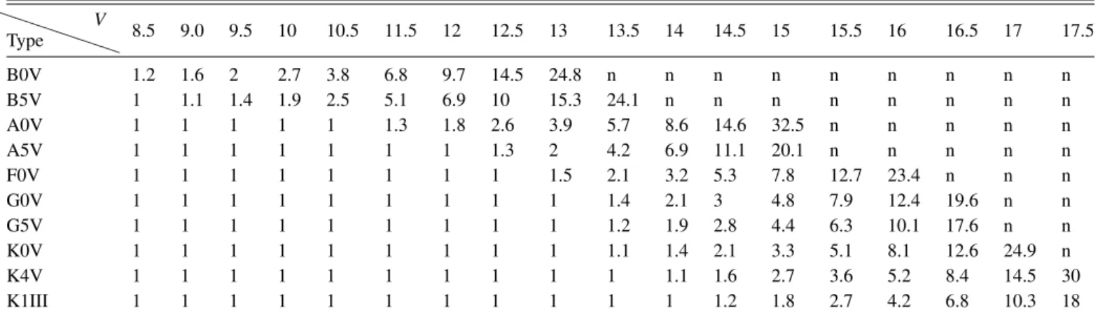
CU6 tables (see Table 1) using the stars’ physical parameters and apparent magnitude are used to obtain σVr. They were com-puted following the prescriptions ofKatz et al.(2004) and later updates. Those tables have been provided for one and 40 field-of-view transits, therefore the value for 40 transits is used here to calculate the average end-of-mission errors in RVS.
Given the information on the apparent Johnson V magnitude and the atmospheric parameters of each star (from the UM), we select from Table1the closest spectral type and return the corresponding radial velocity error. Since Table1 is given for [Fe/H]= 0 alone, a correction is made on the apparent magni-tude in order to take different metallicities into account: for each variation in metallicity of∆[Fe/H] = 1.5 dex, the magnitude is increased by V= 0.5 mag.
We have set a lower limit on the wavelength calibration error, giving a lower limit on the radial velocity error of 1 km s−1. For
the faintest stars the spectra will be of poor quality and will not contain enough information to enable accurate estimation of the radial velocity. Owing to the limited bandwidth in the downlink of Gaia data to Earth, poor quality spectra will not be transmit-ted. We therefore set an upper limit on the radial velocity error of 20 km s−1, beyond which we assume that there will be no data.
The exact point at which the data will be assumed to have too low a quality is still unknown.
3.3.4. Physical parameters
GOG uses the stellar parametrisation performance given by CU8 to calculate error estimations for effective temperature,
Table 1. Average end-of-mission formal error in radial velocity with an assumed average of 40 field-of-view transits, in km s−1, for each spectral type. P P P P P P Type V 8.5 9.0 9.5 10 10.5 11.5 12 12.5 13 13.5 14 14.5 15 15.5 16 16.5 17 17.5 B0V 1.2 1.6 2 2.7 3.8 6.8 9.7 14.5 24.8 n n n n n n n n n B5V 1 1.1 1.4 1.9 2.5 5.1 6.9 10 15.3 24.1 n n n n n n n n A0V 1 1 1 1 1 1.3 1.8 2.6 3.9 5.7 8.6 14.6 32.5 n n n n n A5V 1 1 1 1 1 1 1 1.3 2 4.2 6.9 11.1 20.1 n n n n n F0V 1 1 1 1 1 1 1 1 1.5 2.1 3.2 5.3 7.8 12.7 23.4 n n n G0V 1 1 1 1 1 1 1 1 1 1.4 2.1 3 4.8 7.9 12.4 19.6 n n G5V 1 1 1 1 1 1 1 1 1 1.2 1.9 2.8 4.4 6.3 10.1 17.6 n n K0V 1 1 1 1 1 1 1 1 1 1.1 1.4 2.1 3.3 5.1 8.1 12.6 24.9 n K4V 1 1 1 1 1 1 1 1 1 1 1.1 1.6 2.7 3.6 5.2 8.4 14.5 30 K1III 1 1 1 1 1 1 1 1 1 1 1 1.2 1.8 2.7 4.2 6.8 10.3 18
Notes. The numbers in the top row are Johnson apparent V magnitudes. Fields marked by “n” are assumed to be too faint to produce spectra with sufficient quality for radial velocity determination. Stars with these magnitudes will have no radial velocity information.
line-of-sight extinction, metallicity, and surface gravity. The colour-independent extinction parameter A0 is used in
prefer-ence to the band specific extinctions AV or AG, because A0 is
a property of the interstellar medium alone (Bailer-Jones 2011). CU8 use three different algorithms to calculate physical param-eters using spectrophotometry (seeLiu et al. 2012).
It should be noted that the errors calculated here are calcu-lated only as a function of apparent magnitude. However, as de-scribed inLiu et al.(2012), there are clear dependencies on the spectral type of the star, because some star types may or may not exhibit spectral features required for parameter determina-tion. Additionally, Liu et al. (2012) report a strong correlation between the estimation of effective temperature and extinction. This correlation is not simulated in GOG. Following the recom-mendation of CU8, calculating errors of physical parameters de-pends on apparent magnitude and is split into two cases, objects with A0< 1 mag and A0≥ 1 mag.
In GOG, σTeff, σA0, σFe/H and σlog g are calculated from a Gamma distribution, with shape parameter α and scale parame-ter θ :
f(σ; α, θ)= 1 Γ(σ)θασ
α−1
e−θx (4)
where α and θ are obtained from the following expressions, which have been calculated to give each σ a close approxima-tion to the CU8 algorithm results. A gamma distribuapproxima-tion was selected for ease of implementation and for its ability to statis-tically recreate the CU8 results to a reasonable approximation. A gamma distribution is also only non-zero for positive values of sigma. This is essential when modelling errors because, of course, it is impossible to have a negative error.
– For stars with A0< 1 mag:
αA0 = 0.204 − 0.032G + 0.001G 2 αlog g= 0.151 − 0.019G + 0.001G2 αFe/H= 0.295 − 0.047G + 0.002G2 αTeff = 78.2 − 10.3G + 0.46G2 θA0 = 0.084 θlog g = 0.160 θFe/H= 0.121 θTeff = 28.2.
– For stars with A0≥ 1 mag:
αA0= 0.178 − 0.026G + 0.001G 2 αlog g= 0.319 − 0.044G + 0.002G2 αFe/H= 0.717 − 0.115G + 0.005G2 αTeff = 67.3 − 7.85G + 0.35G 2 θA0 = 0.096 θlog g= 0.179 θFe/H= 0.353 θTeff = 33.5.
The Gamma distributions thus obtained for each parameter are used to generate a formal error for each parameter for each in-dividual star, aiming to statistically (but not inin-dividually) repro-duce the results that will be obtained by the application of the CU8 algorithms and then included in the Gaia Catalogue.
It should be noted that in the stellar parametrisation algo-rithms used inLiu et al. (2012), a degeneracy is reported be-tween extinction and effective temperature owing to the lack of resolved spectral lines only sensitive to effective temperature. In GOG, this degeneracy has not been taken into account, and the precisions of each of the four stellar parameters is simulated in-dependently.
Additionally, the results ofLiu et al. (2012) have recently been updated, andBailer-Jones et al.(2013) gives the latest re-sults regarding the capabilities of physical parameter determi-nation. This latest paper has not been included in the current version of GOG.
3.4. Limitations
In the present paper, only the results for single stars are given in detail. All of the figures and tables represent the numbers and statistics of only individual single stars, excluding all binary and multiple systems. Since the performance of the Gaia satellite is largely unknown for binary and multiple systems, the implemen-tation into GOG of realistic error models has not yet been possi-ble. While the results presented in Sect.5are expected to be reli-able under current assumptions for the performance of Gaia, the real Gaia Catalogue will differ from these results thanks to the presence of binary and multiple systems. By removing binaries from the latter, direct comparison of the results presented here with the real Gaia Catalogue will not be possible because of the presence of unresolved binaries, which are difficult to detect. As a simulator, GOG relies heavily on all inputs and assumptions supplied both from the UM or from the Gaia predicted perfor-mance and error models.
In our simulations we used an exact cut at G = 20 mag, be-yond which no stars are observed. In reality, in regions of low density observations of stars up to 20.5 mag could be possi-ble. Inversely, very crowded regions may not be complete up to 20 mag, or the numbers of observations per star over the five-year mission may be reduced in these regions.
There is no simulation of the impact of crowding on object detection or the detection of components in binary and multiple systems. This can lead to unrealistic quality in all observed data in the most crowded regions of the plane of the Galaxy, to over-estimates for star counts in the bulge, and to a lack of features related to the disk and bulge in Figs.3and19.
Additionally, GOG uses the nominal Gaia scanning law to calculate the number of field of view transits per object over the five years of the mission while Gaia is operating in normal mode. There will be an additional one-month period at the start of the mission using an ecliptic pole scanning law, and this has not been taken into account. It may lead to a slight underestimation of the number of transits, and therefore a slight overestimation of errors, for some stars near the ecliptic poles.
There is the possibility that the Gaia mission will be ex-tended above the nominal five-year mission. Since this idea is under discussion and has not yet been confirmed or dis-carded, we only present results for the Gaia mission as originally planned.
If the length of the mission is increased, the number of field-of-view transits will increase, and the precision per object will improve. If the proposal is accepted, the GOG simulator could be used to provide updated statistics for the expected catalogue without extensive modification.
4. Methods and statistics
Considering current computing capabilities, it is not straightfor-ward to make statistics and visualisations when dealing with cat-alogues of such a large size. A specific tool has been created which is capable of extracting information and visualising re-sults, with excellent scalability allowing its use for huge datasets and distributed computing systems.
The Gaia Analysis Tool (GAT) is a data analysis package that allows, through three distinct frameworks, generation of statistics, validation of data, and generation of catalogues. It cur-rently handles both UM- and GOG-generated data, and could be adapted to handle other data types.
Every statistical analysis is performed by a Statistical Analysis Module (SAM), with several grouped into a single
XML file as an input to GAT. Each SAM can contain a set of fil-ters, enabling analysis of specific subsets of the data. This allows the production of a wide range of statistics for objects satisfying any number of specific user-defined criteria or for the catalogue as a whole.
GAT creates a number of different statistics outputs includ-ing histograms, sky density maps and HR diagrams. After the GAT execution, statistics output are stored to either generate a report or to be analysed using the GAT Displaying tool.
Because we have information from not only observations of a population but also of the observed population itself, compar-ison is possible between the simulated Gaia Catalogue and the simulated “true” population, allowing large scope for investigat-ing the precision3 of the observations and differences between
the two catalogues. Clearly this is only possible with simulated data and cannot be attempted with the true Gaia Catalogue, so it is an effective way to investigate the possible extent and ef-fect of observational errors and selection bias on the real Gaia Catalogue, where this kind of comparison is not possible.
GOG can be used in the preparations for validating the true GaiaCatalogue, by testing the GOG catalogue for accuracy3and precision. In special cases, observational biases could even be implemented into the code to allow thorough testing of valida-tion methods.
5. Results
The GOG simulator has been used to generate the simulated fi-nal mission catalogue for Gaia, down to magnitude G= 20. The simulation was performed on the MareNostrum super computer at the Barcelona Supercomputing Centre (Centre Nacional de Supercomputació), and it took 400 thousand CPU hours. An ex-tensive set of validations and statistics have been produced using GAT to validate performance of the simulator. Below we include a subset of these statistics for the most interesting cases to give an overview of the expected Gaia Catalogue.
5.1. General
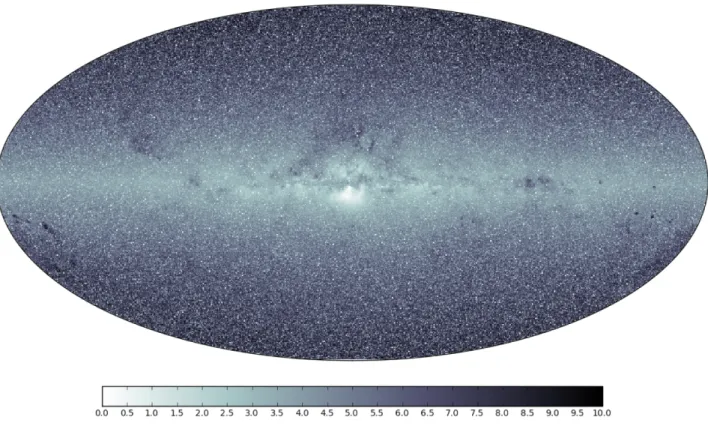
In total, GOG has produced a catalogue of about one billion objects, consisting of 523 million individual single stars and 484 million binary or multiple systems. The total number of stars, including the components of binary and multiple systems is 1.6 billion. The skymap of the total flux detected over the en-tire five-year mission is given in Fig.1. Although GOG can pro-duce extragalactic sources, none have been simulated here.
The following discussion is split into sections for different types of objects of interest. Section5.2covers all Galactic stellar sources. Section5.3covers all variable objects. Section5.4is a discussion of physical parameters estimated by Gaia. All objects in these sections are within the Milky Way.
To make the presentation of performance as clear as possible, all binary and multiple systems and their components have been removed from the following statistics. This is due to complicat-ing effects that arise when dealing with binary systems, some of which GOG is not yet capable of correctly simulating; for example, GOG does not yet contain an orbital solution in its as-trometric error models, and the effects of unresolved systems 3 Here we assume the standard definition of accuracy and precision:
accuracy is the closeness of a result (or set) to the actual value, i.e. it is a measure of systematics or bias. Precision is the extent of the random variability of the measurement, i.e. what is called observational errors above.
Fig. 1.Skymap of total integrated flux over the Milky Way, in the G band. The colour bar represents a relative scale, from maximum flux in white to minimum flux in black. The figure is plotted in Galactic coordinates with the Galactic-longitude orientation swapped left to right.
on photometry and astrophysical parameter determination have not yet been well determined. Therefore, the numbers presented are only for individual single stars and do not include the full one billion objects simulated. Of the single stars presented in this paper, 74 million are within the radial velocity spectrometer magnitude range.
Table2gives the mean and median error for each of the ob-served parameters discussed in this paper, along with the upper and lower 25% quartile.
In Fig.2, the mean error for parallax, position, proper mo-tion, and photometry in the four Gaia bands are given as a func-tion of G magnitude. Also, the mean error in radial velocity is given as a function of GRVSmagnitude. The sharp jumps in the
mean error in astrometric parameters between 8 and 12 mag are due to the activation of gates for the brighter sources in an at-tempt to prevent CCD saturation (see Sect.3.3.1).
5.2. Stars 5.2.1. Parallax
The distribution of parallax measurements for all single stars is given in Fig. 4. The mean parallax error for all single stars is 147.0 µas. The number of single stars falling below three rela-tive parallax error limits is given in Table3for each spectral type and in Table4for each luminosity class. For those interested in a specific type of star, Table 5gives the full breakdown of the number of single stars falling below three relative parallax error limits for every spectral type and luminosity class. The distri-bution of parallax errors is given for each stellar population in Fig.5and for each spectral type in Fig.7. The relative parallax error σ$/$ is given in Fig.6for stars split by spectral type.
Table 2. Mean and median value of the end-of-mission error in each observable, along with the upper (UQ) and lower (LQ) 25% quartile.
Standard error LQ Median Mean UQ
Parallax (µas) 80 140 147 210 α∗ (µas) 40 80 91 130 δ (µas) 50 100 103 150 µα(µas yr−1) 40 80 82 120 µδ(µas yr−1) 40 70 73 110 G(mmag) 2 3 3.0 4 GBP(mmag) 6 11 14.6 19 GRP(mmag) 5 7 7.7 10 GRVS(mmag) 6 11 13.2 18 Radial velocity (km·s−1) 3 7 8.0 13 Extinction (mag) 0.16 0.21 0.21 0.26 Metallicity (Fe/H) 0.46 0.57 0.57 0.73
Surface gravity (log g) 0.34 0.35 0.45 0.58
Effective temperature (K) 280 350 388 530
Notes. Since the error distributions are not symmetrical, the mean value should not be used directly, and is given only to give an idea of the approximate level of Gaia’s precision. The median G magnitude of all single stars is 18.9 mag.
The error in parallax measurements for Gaia depends on the magnitude of the source, the number of observations made, and the true value of the parallax. Figure3 shows the mean paral-lax error over the sky. Its shape clearly follows that of the Gaia scanning law. The red area corresponding to the region of worst precision is due to the bulge population, which suffers from high levels of reddening. The faint ring around the centre of the figure
6 8 10 12 14 16 18 20 G magnitude [mag] 0 100 101 102 103 Mean error [µ as] $ α δ 6 8 10 12 14 16 18 20 G magnitude [mag] 0 100 101 102 103 Mean error [µ as yr − 1] µα µδ 6 8 10 12 14 16 18 20 G magnitude [mag] 0 100 101 102 Mean error [mmag] GGBP GRP GRVS 6 8 10 12 14 16 GRV Smagnitude [mag] 1 2 3 4 5 6 7 8 9 10 Mean error [km s − 1] Radial velocity
Fig. 2.Mean end-of-mission error as a function of G magnitude for parallax, position, proper motion, and photometry in the four Gaia passbands.
Additionally the mean end-of-mission error in radial velocity as a function of GRVSmagnitude.
Fig. 3.Sky map (healpix) of mean parallax error for all single stars in
equatorial coordinates. Colour scale is mean parallax error in µas. The red area is the location of the bulge.
corresponds to the disk of the Galaxy, remembering that the plot is given in equatorial coordinates. The blue areas corresponding to regions of improved mean precision are areas with a higher number of observations. The characteristic shape of this plot is due to the Gaia scanning law. The error in parallax as a function of measured G magnitude is given in Fig.8and as a function of the real parallax in Fig.9.
−2000 0 2000 4000 6000 8000 10000 Parallax [µas] 0 100 101 102 103 104 105 106 107 108 Coun t All stars
Fig. 4.Histogram of parallax for all single stars. The histogram contains
99.5% of all data.
5.2.2. Position
Gaiawill be capable of measuring the position of each observed star at an unprecedented accuracy, producing the most precise full sky position catalogue to date.
The mean error is 90 µas for right ascension and 103 µas for declination. The distribution of error in right ascension and
Table 3. Total number of single stars for each spectral type, along with the percentage of those that fall below each relative parallax error limit; e.g., 68% of M-type stars have a relative parallax error better than 20%.
Spec. type Total σ$/$ < 1 σ$/$ < 0.2 σ$/$ < 0.05
O 3.3 × 10² 87.5 57.5 29.2 B 3.4 × 10⁵ 74.0 33.0 12.2 A 5.3 × 10⁶ 79.7 38.0 14.7 F 1.2 × 10⁸ 66.2 20.1 6.1 G 2.0 × 10⁸ 67.4 20.0 5.7 K 1.5 × 10⁸ 82.4 30.9 8.6 M 4.5 × 10⁷ 98.1 68.0 18.6
Table 4. Total number of single stars for each luminosity class, along with the percentage that fall below each relative parallax error limit.
Lum. class Total σ$/$ < 1 σ$/$ < 0.2 σ$/$ < 0.05
Supergiant 5.6 × 10³ 91.5 65.9 36.8 Bright giant 6.9 × 10⁵ 87.1 57.9 25.1 Giant 6.6 × 10⁷ 67.5 21.4 7.0 Sub-giant 7.5 × 10⁷ 60.2 16.8 5.3 Main sequence 3.8 × 10⁸ 78.1 30.7 8.5 White dwarf 2.1 × 10⁵ 100.0 94.3 41.9
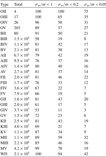
Table 5. Total number of single stars for each stellar classification, along with the percentage that fall below each relative parallax error limit. Type Total σ$/$ < 1 σ$/$ < 0.2 σ$/$ < 0.05 OII 4 100 100 75 OIII 17 100 65 35 OIV 26 96 50 31 OV 203 89 57 27 BII 80 91 50 21 BIII 1.5 × 10⁵ 58 19 8 BIV 1.1 × 10⁵ 81 42 17 BV 2.1 × 10⁵ 81 38 13 AII 6.7 × 10³ 79 42 19 AIII 9.5 × 10⁵ 76 37 16 AIV 1.4 × 10⁶ 80 40 16 AV 2.7 × 10⁶ 81 37 14 FII 2.0 × 10³ 81 46 22 FIII 1.7 × 10⁶ 76 33 12 FIV 3.6 × 10⁷ 67 22 7 FV 7.9 × 10⁷ 66 19 5 GII 1.6 × 10⁵ 81 43 20 GIII 2.0 × 10⁷ 61 17 5 GIV 3.7 × 10⁷ 53 11 3 GV 1.5 × 10⁸ 72 23 6 KII 2.5 × 10⁵ 81 43 19 KIII 4.0 × 10⁷ 69 21 7 KV 1.1 × 10⁸ 87 34 9 MII 1.1 × 10⁴ 89 59 32 MIII 2.2 × 10⁶ 85 46 16 MV 4.2 × 10⁷ 99 70 19 WD 2.1 × 10⁵ 100 94 42 0 100 200 300 400 500
Error in Parallax [µas]
0 100 101 102 103 104 105 106 107 Coun t All Thin Disk Thick Disk Halo Bulge
Fig. 5.Histogram of end-of-mission parallax error for all single stars,
split by stellar population.
0.0 0.2 0.4 0.6 0.8 1.0
Relative error in Parallax [σ$/$] 0 100 101 102 103 104 105 106 107 108 109 Cum ulativ e Coun t All O type B type A type F type G type K type M type White Dwarf
Fig. 6.Cumulative histogram of relative parallax error for all single
stars, split by spectral type. The histogram range displays 74% of all data.
0 100 200 300 400 500
Parallax Error [µas]
0 100 101 102 103 104 105 106 107 Coun t All O type B type A type F type G type K type M type White Dwarf
Fig. 7.Histogram of end-of-mission parallax error for all single stars,
6 8 10 12 14 16 18 20 G magnitude [mag] 50 100 150 200 250 300 350 400 450 P arallax error [µ as] 0.0 0.5 1.0 1.5 2.0 2.5 3.0 3.5 4.0 4.5 5.0 5.5
Fig. 8.End-of-mission parallax error against G magnitude for all single
stars. The colour scale represents the log of density of objects in a bin size of 80 mmag by 2.5 µas. White area represents zero stars.
250 500 750 1000 1250 1500 1750
Real parallax [µas] 40 80 120 160 200 240 280 320 360 400 440 480 P arallax Error [µ as] 0.0 0.5 1.0 1.5 2.0 2.5 3.0 3.5 4.0 4.5 5.0
Fig. 9.End-of-mission parallax error against parallax for all single stars.
The colour scale represents the log of density of objects in a bin size of 10 by 2.5 µas. White area represents zero stars.
declination as a function of the true value, along with a his-togram of the error, are given in Figs.10and11. The overdensi-ties are due to the bulge of the Galaxy.
5.2.3. Proper motion and radial velocity
In addition to parallax measurements, Gaia will also measure proper motions for all stars it detects. The proper motion in right ascension and declination is labelled as µαand µδ, respectively. The mean error in µαis 81.7 µas yr−1, and in µδis 72.9 µas yr−1.
0 50 100 150 200 250 300 350 Real right ascension [deg] 0 50 100 150 200 250 300 350 400 450 Righ t ascension Error [µ as] 0 28 56 Count 0 32 64 96 128 160 Coun t 0.0 0.2 0.4 0.6 0.8 1.0 1.2 1.4 1.6 1.8
Fig. 10.Right ascension error against real right ascension. The colour
scale is linear, with a factor of 105. Histograms are computed for both
right ascension and right ascension error. The colour scale represents log density of objects in a bin size of 2 degrees by 7.5 µas. White area represents zero stars.
−50 0 50
Real declination [deg] 0 50 100 150 200 250 Declination Error [µ as] 0 21 42 Count 0 22 44 66 88 110 Coun t 0.0 0.2 0.4 0.6
Fig. 11.Declination error against real declination. The colour scale is
linear, with a factor of 105. Histograms are computed for both
decli-nation and declidecli-nation error. The colour scale represents log density of objects in a bin size of 1 degrees by 5 µas. White area represents zero stars.
The distribution of errors in both components of proper motion is given in Fig.12.
The radial velocity is measured by the on-board radial ve-locity spectrometer. This instrument is only sensitive to stars down to GRVS = 17 mag. We assume an upper limit on the
0 50 100 150 200 250 300 Proper motion error [µas yr−1]
0 100 101 102 103 104 105 106 107 Coun t µα µδ
Fig. 12.Error in proper motion for alpha and delta for all single stars.
0 5 10 15 20
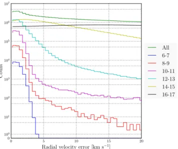
Radial velocity error [km s−1] 0 100 101 102 103 104 105 106 107 Coun t All 6-7 8-9 10-11 12-13 14-15 16-17
Fig. 13.Histogram of radial velocity error split by G magnitude range.
The histogram contains 100% of all data that have radial velocity information.
precision worse than this will not be given any radial velocity information.
Of the 523 million measured individual Milky Way stars, 74 million have a radial velocity measurement. The mean error in the radial velocity measurement is 8.0 km s−1. The distribution of radial velocity error is given for each G magnitude in Fig.13, and in Fig.14split by spectral type. The radial velocity error is given as a function of GRVSmagnitude in Fig.16.
5.2.4. Photometry
The end-of-mission error in each measurement as a function of Gmagnitude is given in Fig.17.
Gaiawill produce low-resolution spectra, in addition to mea-suring the magnitude of each source in the Gaia bands G, GBP,
GRP, and GRVS. Whilst GOG is capable of simulating these
spec-tra, they have not been included in the present simulations owing to the long computation time and the large storage space require-ment of a catalogue of spectra for one billion sources.
0 5 10 15 20
Radial velocity error [km s−1] 0 100 101 102 103 104 105 106 107 Coun t All O B A F G K M
Fig. 14. Histogram of radial velocity error split by spectral type.
The histogram contains 100% of all data that have radial velocity information.
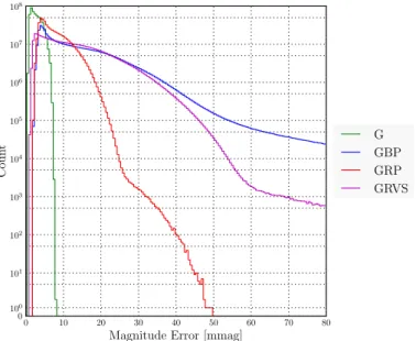
Figure18shows the distribution in the error of each photo-metric measurement. As can be seen in this figure, the error in Gis much lower than for the other instruments, and for all stars it is less than 8 mmag. The mean error in G is 3.0 mmag. The mean error in GBPand GRPis 14.6 mmag and 7.7 mmag,
respec-tively. The mean error in GRVSis 13.2 mmag, although it must
be remembered that the radial velocity spectroscopy instrument is limited to brighter than GRVS= 17.
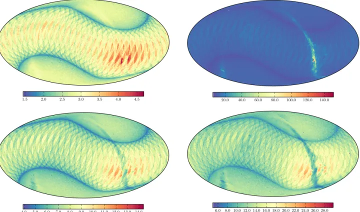
Figure19shows the mean photometric error as a function of position on the sky for the four Gaia photometric passbands. The structure seen in all four maps is derived from the Gaia scanning law.
It is interesting to point out the ring in the four plots of Fig.19caused by the disk of the Galaxy. Owing to significant levels of interstellar dust in the disk of the Galaxy, visible ob-jects are generally much redder. This reddening causes obob-jects to lose flux at the bluer end of the spectrum, making them ap-pear fainter to the GBP photometer. Therefore the plane of the
Galaxy can be seen as an increase in the mean photometric error in the GBPerror map.
Conversely, the disk of the Galaxy shows as a ring of de-creasedmean photometric error in the GRPand GRVSmaps, since
the sensitivity of their spectra is skewed more towards the red-der end of the spectrum. It is important to note, however, that the effect of crowding on photometry is not accounted for in GOG.
5.3. Variables
Gaiawill be continuously imaging the sky over its full five-year mission, and each individual object will be observed 70 times on average. The scanning law means that the time between re-peated observations varies, and Gaia will be incredibly useful for detecting many types of variable stars. GOG produces a to-tal of 10.8 million single variable objects. This number comes from the UM (Robin et al. 2012) and assumes 100% variability detection. The exact detection rates and the classification accu-racy for each variability type are still unknown. In fact, the num-bers of variable objects in the catalogue is expected to be higher than 10.8 million because some variable star types have not yet
6 8 10 12 14 16 18 20 G magnitude [mag] 50 100 150 200 250 µα Error [µ as yr −1] 0.0 0.5 1.0 1.5 2.0 2.5 3.0 3.5 4.0 4.5 5.0 5.5 6 8 10 12 14 16 18 20 G magnitude [mag] 50 100 150 200 250 µδ Error [µ as yr − 1] 0.0 0.5 1.0 1.5 2.0 2.5 3.0 3.5 4.0 4.5 5.0 5.5 6.0
Fig. 15.2D histograms showing error in proper motion against G magnitude. The colour scale represents the log density of objects in a bin size of
80 mmag by 2 µas yr−1. Left is proper motion in right ascension, and right is proper motion in declination. White area represents zero stars.
10 11 12 13 14 15 16 17 GRV Smagnitude [mag] 2 4 6 8 10 12 14 16 18 20 Radial V elo cit y Error [km s − 1] 0.0 0.5 1.0 1.5 2.0 2.5 3.0 3.5 4.0
Fig. 16.End-of-mission error in radial velocity against GRVSmagnitude.
The colour scale represents the log density in a bin size of 50 mmag by 1 km s−1. White area represents zero stars.
been implemented (see Robin et al. 2012 for a more detailed description).
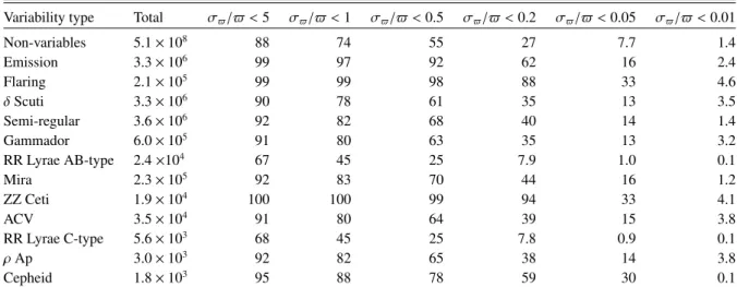
The distribution of relative parallax error is given for each type of variable star in Fig. 20. The numbers of each type of variable produced by GOG are given in Table6, along with the number of each type that falls below each relative parallax error limit.
In general, the numbers of variables presented in this paper are lower than inRobin et al.(2012) by a factor of two or three. This is expected, because in the present paper we are exclud-ing all variables that are part of binary or multiple systems, and presenting the number of single variable stars alone.
However, the number of emission variables is higher in the present paper. This is due to implementation of new types of emission stars: Oe, Ae, dMe, and WR stars. These are now in-cluded as emission variables but were not simulated inRobin et al.(2012). Additionally, the number of Mira variable stars is higher in the present paper. This is from an implementation error in the version of the UM used inRobin et al.(2012), which has been fixed in the version used in the present paper.
5.3.1. Cepheids and RR-Lyrae
Cepheids and RR-Lyrae are types of pulsating variable stars. Their regular pulsation and a tight period–luminosity relation make them excellent standard candles, and therefore of particu-lar interest in studies of Galactic structure and the distance scale. Figure21shows the histogram of error in parallax specifically for Cepheid and RR-Lyrae variable stars, while Fig.22shows the errors in proper motions for Cepheids and RR-Lyrae. 5.4. Physical parameters
Adding low-resolution spectral photometers on-board Gaia will make it capable of providing information on several object pa-rameters including an estimate of line-of-sight extinction, e ffec-tive temperature, metallicity, and surface gravity. Discussion of each individual physical parameter is given below.
Provided here are results for an approximation of the results ofLiu et al.(2012), which reproduces CU8 results statistically but not individually for each star. Therefore for detailed analysis of specific object types, care should be taken. Again, due to the very long tails of the error distributions caused by large numbers of extremely faint stars, the mean values given below should be taken with caution.
5.4.1. Extinction
Across many fields of astronomy, the effects of extinction on the apparent magnitude and colour of stars can play a major role in contributing to uncertainty. An accurate estimation of
6 8 10 12 14 16 18 20 G [mag] 10 20 30 40 G Error [mmag] 6 8 10 12 14 16 18 20 G [mag] 10 20 30 40 GBP Error [mmag] 6 8 10 12 14 16 18 20 G [mag] 10 20 30 40 GRP Error [mmag] 6 8 10 12 14 16 18 20 G [mag] 10 20 30 40 GR VS Error [mmag] 0.00 0.50 1.00 1.50 2.00 2.50 3.00 3.50 4.00 4.50 5.00 5.50 6.00 6.50
Fig. 17.End-of-mission errors in photometry as a function of G magnitude. The colour scale represents the log density of objects in a bin size of
80 mmag by 0.4 mmag. Top left, G magnitude; top right, GBP; bottom left, GRP; bottom right, GRVS. White area represents zero stars.
0 10 20 30 40 50 60 70 80
Magnitude Error [mmag] 0 100 101 102 103 104 105 106 107 108 Coun t GGBP GRP GRVS
Fig. 18.Histogram of error in G, GRVS, GRP, and GBPfor all single stars.
extinction will prove highly useful for many applications of the GaiaCatalogue.
Figure23shows the comparison between true extinction and the simulated Gaia estimate. For the vast majority of stars, the Gaiaestimated extinction lies very close to the true value. This could prove very useful when, for example, using parallax and apparent magnitude data from Gaia because accurate extinction estimates are required to constrain the absolute magnitude of an object.
Additionally, these results show that the Gaia data will be highly useful in terms of mapping Galactic extinction in three dimensions, thanks to the combination of a large number of ac-curate parallax and extinction measurements. The negative ex-tinction values in Fig. 23 are of course non-physical and are simply the result of applying a Gaussian random error to stars with near zero extinction.
The discontinuity at A0 = 1 in the top left-hand panel of
Fig.23comes from the distinction made between high and low extinction stars in the presentation of the results in Liu et al.
(2012). Our algorithm is based on results given in that paper, where the dependence on the extinction has been simplified to
Fig. 19.HealPixMap in equatorial coordinates of the mean error in: top left: G; top right: GBP; lower left: GRP; lower right: GRVS. The colour scale
gives the mean photometric error in mmag. The colour scales are different due to differences in the maximum mean magnitude.
0.0 0.2 0.4 0.6 0.8 1.0
Relative error in Parallax [σ$/$] 0 100 101 102 103 104 105 106 107 Cum ulativ e Coun t SemiRegular Cepheid DeltaScuti Emmission Flairing Gammador Microlens Mira roAp RRab RRc ACV ZZceti
Fig. 20.Cumulative histogram of the relative parallax error for all single
stars, split by variability type. The histogram range displays 85% of all data.
two cases, stars with A0< 1 and those with A0 > 1. This
distinc-tion was made only for presentadistinc-tion of the results, and the real results from the DPAC algorithms will not show this discontinu-ity.Liu et al.(2012) report a degeneracy between extinction and effective temperature due to the lack of resolved spectral lines sensitive only to effective temperature.
5.4.2. Effective temperature
For all objects in the GOG catalogue, the measured effective temperature ranges between 850 and 102 000 K. The error in
0 100 200 300 400 500
Parallax Error [µas]
0 100 101 102 103 Coun t σ $Cepheid σ$RR-Lyrae
Fig. 21.Histogram of parallax error for Cepheid and RR-Lyrae
vari-able stars. RR-Lyrae is a combination of the two sub-populations RR-ab and RR-c.
effective temperature is less than 640 K for all stars, with a mean value of 388 K. Figure23shows the comparison between true object effective temperature and the Gaia estimation. The thin lines visible in Fig.23are an artefact from the UM, which uses a Hess diagram to produce stars, leading to some quantisation in the effective temperature of simulated stars.
5.4.3. Metallicity
Metallicity can be estimated by Gaia in the form of [Fe/H]. Measured values range from −6.5 to +4.6. The mean error in
Table 6. Total number of single stars of each variability type, and the percentage of each that falls below each relative parallax error limit: 500%, 100%, 50%, 20%, 5%, and 1%.
Variability type Total σ$/$ < 5 σ$/$ < 1 σ$/$ < 0.5 σ$/$ < 0.2 σ$/$ < 0.05 σ$/$ < 0.01
Non-variables 5.1 × 10⁸ 88 74 55 27 7.7 1.4 Emission 3.3 × 10⁶ 99 97 92 62 16 2.4 Flaring 2.1 × 10⁵ 99 99 98 88 33 4.6 δ Scuti 3.3 × 10⁶ 90 78 61 35 13 3.5 Semi-regular 3.6 × 10⁶ 92 82 68 40 14 1.4 Gammador 6.0 × 10⁵ 91 80 63 35 13 3.2 RR Lyrae AB-type 2.4 ×10⁴ 67 45 25 7.9 1.0 0.1 Mira 2.3 × 10⁵ 92 83 70 44 16 1.2 ZZ Ceti 1.9 × 10⁴ 100 100 99 94 33 4.1 ACV 3.5 × 10⁴ 91 80 64 39 15 3.8 RR Lyrae C-type 5.6 × 10³ 68 45 25 7.8 0.9 0.1 ρ Ap 3.0 × 10³ 92 82 65 38 14 3.8 Cepheid 1.8 × 10³ 95 88 78 59 30 0.1 0 50 100 150 200 250 300
Proper Motion Error [µas]
0 100 101 102 103 Coun t σµαCepheid σµαRR-Lyrae σµδCepheid σµδRR-Lyrae
Fig. 22.Histogram of proper motion error µαand µδ for Cepheid and
RR-Lyrae variable stars. RR-Lyrae is a combination of the two sub-populations RR-ab and RR-c.
metallicity estimate is 0.57 dex. The relatively high error in metallicity estimate can lead a large difference between real and observed values, as seen in Fig.23.
5.4.4. Surface gravity
The mean error in surface gravity is 0.45 dex. The comparison between real and observed surface gravity can be seen in Fig.23. As with metallicity, the lines at regular intervals at high gravity in this plot are due to the UM (Robin et al. 2012).
6. Conclusions
The Gaia Object Generator provides the most complete pic-ture to date of what can be expected from the Gaia astromet-ric mission. Its simulated catalogue provides useful insight into how various types of objects will be observed and how each of their observables will appear after including observational errors and instrument effects. The simulated catalogue includes directly
observed quantities, such as sky position and parallax, as well as derived quantities, such as interstellar extinction and metallicity. Additionally, the full sky simulation described here is useful for gaining an idea of the size and format of the eventual Gaia Catalogue, for preparing tools and hardware for hosting and dis-tribution of the data, and for becomeing familiar with working with such a large and rich dataset.
In addition to the stellar simulation described in this paper, there are plans to generate other simulated catalogues of interest, such as open clusters, Magallanic Clouds, supernovae, and other types of extragalactic objects, so that a more complete version of the simulated Gaia Catalogue can be compiled.
Here we have focused on the simulated catalogue from the inbuilt Gaia Universe Model, based on the Besançon Galaxy model. However, GOG can alternatively be supplied with an in-put catalogue generated by the user. This way, simulated data from any other model can be processed with GOG to obtain simulated Gaia observations of specific interest to the individ-ual user. The input can be either synthetic data on a specific star or catalogue, or an entire simulated survey such as those gener-ated using Galaxia (Sharma et al. 2011), provided a minimum of input information is supplied (e.g. position, distance, apparent magnitude, and colour).
With GOG, the capabilities of the instrument can be ex-plored, and it is possible to gain insight into the expected per-formance for specific types of objects. While only a subset of the available statistics have been reproduced here, it is possible to obtain the full set of available statistics at request.
We are working to make the full simulated catalogue pub-licly available, so that interested individuals can begin working with data similar to the forthcoming Gaia Catalogue.
Acknowledgements. GOG is the product of many years of work from a number of people involved in DPAC and specifically CU2. The authors would like the thank the various CUs for contributing predicted error models for Gaia. The pro-cessing of the GOG data made significant use of the Barcelona Supercomputing Center (MareNostrum), and the authors would specifically like to thank Javi Castañeda, Marcial Clotet, and Aidan Fries for handling our computation and data handling needs. Additionally, thanks go to Sergi Blanco-Cuaresmo for his help with Matplotlib. This work was supported by the Marie Curie Initial Training Networks grant number PITN-GA-2010-264895 ITN “Gaia Research for European Astronomy Training”, and MINECO (Spanish Ministry of Economy) - FEDER through grants AYA2009-14648-C02-01, AYA2010-12176-E, AYA2012-39551-C02-01, and CONSOLIDER CSD2007-00050.
−1 0 1 2 3 4 5 6 7 8 Observed extinction [A0] 0 1 2 3 4 5 6 7 8 Real extinction [A0 ] 4 6 Count [log] 2 4 6 8 Coun t [log ] 0.0 0.5 1.0 1.5 2.0 2.5 3.0 3.5 4.0 4.5 5.0 5.5 6.0 −4 −3 −2 −1 0 1 2 3 4
Observed metalicity [Fe/H] −4 −3 −2 −1 0 1 2 3 4 Real metalicit y [F e/H] 0 4 8 Count [log] 2 4 6 8 Coun t [log ] 0.0 0.5 1.0 1.5 2.0 2.5 3.0 3.5 4.0 4.5 5.0 5.5 0 2 4 6 8 10
Observed log gravity [log g] 0 2 4 6 8 10 Real log gra vit y [log g] 0 4 8 Count [log] 2 3 4 5 6 7 8 Coun t [log ] 0.0 0.5 1.0 1.5 2.0 2.5 3.0 3.5 4.0 4.5 5.0 5.5 6.0 6.5 0 2000 4000 6000 8000 10000 12000 14000 16000 Observed effective temperature [K] 0 2000 4000 6000 8000 10000 12000 14000 16000 Real effectiv e temp erature [K] 0 4 8 Count [log] 2 4 6 8 Coun t [log ] 0.0 0.5 1.0 1.5 2.0 2.5 3.0 3.5 4.0 4.5 5.0 5.5 6.0 6.5
Fig. 23.Comparison of the true values of physical parameters with the GOG “observed” values for: top left, extinction; top right, metallicity;
bottom left, surface gravity; and bottom right, effective temperature. The colour scales represent log density of objects in a bin size of: top left, 50 by 50 mmag; top right, 0.4 by 0.4 dex; bottom left, 0.5 by 0.5 dex; and bottom right, 100 by 100 K. White area represents zero stars.
References
Babusiaux, C. 2005, in The Three-Dimensional Universe with Gaia, eds. C. Turon, K. S. O’Flaherty, & M. A. C. Perryman, ESA SP, 576, 417 Bailer-Jones, C. A. L. 2011, MNRAS, 411, 435
Bailer-Jones, C. A. L., Andrae, R., Arcay, B., et al. 2013, A&A, 559, A74 de Bruijne, J. H. J. 2012, Ap&SS, 341, 31
Isasi, Y., Figueras, F., Luri, X., & Robin, A. C. 2010, in Highlights of Spanish Astrophysics V, eds. J. M. Diego, L. J. Goicoechea, J. I. González-Serrano, & J. Gorgas (Heidelberg, Berlin: Springer-Verlag), 415
Jordi, C., Gebran, M., Carrasco, J. M., et al. 2010, A&A, 523, A48 Katz, D., Munari, U., Cropper, M., et al. 2004, MNRAS, 354, 1223
Liu, C., Bailer-Jones, C. A. L., Sordo, R., et al. 2012, MNRAS, 426, 2463 Masana, E., Isasi, Y., Luri, X., & Peralta, J. 2010, in Highlights of Spanish
Astrophysics V, eds. J. M. Diego, L. J. Goicoechea, J. I. González-Serrano, & J. Gorgas (Heidelberg, Berlin: Springer-Verlag), 515
Perryman, M. A. C., & ESA 1997, The H and Tycho cata-logues. Astrometric and photometric star catalogues derived from the ESA HSpace Astrometry Mission ESA SP (Noordwijk: ESA), 1200 Perryman, M. A. C., de Boer, K. S., Gilmore, G., et al. 2001, A&A, 369, 339 Robin, A. C., Reylé, C., Derrière, S., & Picaud, S. 2003, A&A, 409, 523 Robin, A. C., Luri, X., Reylé, C., et al. 2012, A&A, 543, A100