A new approach to stellar occultations in the Gaia era

HAL Id: tel-03185433

https://tel.archives-ouvertes.fr/tel-03185433

HAL is a multi-disciplinary open access archive for the deposit and dissemination of sci-entific research documents, whether they are pub-lished or not. The documents may come from teaching and research institutions in France or abroad, or from public or private research centers.

L’archive ouverte pluridisciplinaire HAL, est destinée au dépôt et à la diffusion de documents scientifiques de niveau recherche, publiés ou non, émanant des établissements d’enseignement et de recherche français ou étrangers, des laboratoires publics ou privés.

Joao Ferreira

To cite this version:

Joao Ferreira. A new approach to stellar occultations in the Gaia era. Astrophysics [astro-ph]. Université Côte d’Azur; Universidade de Lisboa. Faculdade de ciências (Lisboa, Portugal), 2020. English. �NNT : 2020COAZ4084�. �tel-03185433�

Occultations stellaires: une nouvelle

approche grâce à la mission Gaia

João FERREIRA

Laboratoire J-L. Lagrange – Observatoire de la Côte d’Azur ; Instituto de

Astrofísica e Ciências do Espaço, Lisboa

Présentée en vue de l’obtention

du grade de docteur en Sciences de la Planète et de l’Univers

d’Université Côte d’Azur

et de Faculdade de Ciências da Universidade de Lisboa

Dirigée par : Paolo Tanga

Co-encadrée par : Pedro Machado Soutenue le : 2020-12-15

Devant le jury, composé de :

Felipe BRAGA-RIBAS (Universidade Tecnológica Federal do Paraná)

René DUFFARD (Instituto de Astrofisica de Andalucía) Guy LIBOUREL (Université Côte d’Azur)

Pedro MACHADO (Instituto de Astrofísica e Ciências do Espaço)

Françoise ROQUES (Observatoire de Paris)

Pablo SANTOS-SANZ (Instituto de Astrofisica de Andalucía) Paolo TANGA (Observatoire de la Côte d’Azur)

Kleomenis TSIGANIS (Aristotle University of Thessaloniki)

grâce à la mission Gaia

A new approach to stellar occultations in the Gaia era

Jury:

Président du jury :

Guy LIBOUREL, Professeur, Université Côte d’Azur Rapporteurs :

Felipe BRAGA-RIBAS, Professeur Associé, Universidade Tecnológica Federal do Paraná Pablo SANTOS-SANZ, Maître des Conférences, Instituto de Astrofisica de Andalucía Examinateurs:

René DUFFARD, Professeur Associé, Insituto de Astrofisica de Andalucía Françoise ROQUES, Astronome, Observatoire de Paris

Kleomenis TSIGANIS, Professeur Associé, Aristotle University of Thessaloniki Directeur de thèse:

Paolo TANGA, Astronome, Observatoire de la Côte d’Azur Co-Directeur de thèse:

Les astéroïdes participent à la compréhension de plusieurs problèmes clés liés à la science du système solaire et à l’environnement spatial de notre planète, tels que les conditions du système solaire lors de sa formation, l’apport d’eau et de molécules organiques sur la Terre, le danger potentiel des astéroïdes proches de la Terre ("Near Earth Asteroids" - NEA) et leur rôle dans l’influence du climat de la Terre.

Les occultations stellaires sont une occasion unique d’obtenir du sol une astrométrie astéroïde très précise, proche de la performance de Gaia, ainsi que des formes / tailles pour les astéroïdes. Lorsqu’un astéroïde cache la lumière d’une étoile, l’incertitude de sa position instantanée peut être similaire à celle de l’étoile cible. En exploitant la précision de Gaia DR2 sur les astéroïdes et les étoiles, la prédiction et l’exploitation des occultations stellaires deviennent une méthode efficace pour collecter systématiquement l’astrométrie des astéroïdes. L’amélioration des prévisions via Gaia DR2 est prouvée par des statistiques de prévisions réelles et une comparaison entre les prédictions d’occultations stellaires avec Gaia DR2 pour les astéroïdes et autres données, comme Astorb et MPCORB, afin de vérifier lesquelles correspondent le mieux aux cordes observées d’occultations passées.

En même temps, les occultations d’astéroïdes peuvent offrir la possibilité de confirmer ou de découvrir des étoiles doubles, dans une gamme de petites séparations angulaires très complémentaires de la résolution accessible à Gaia elle-même. Nous présenterons des statistiques et des simulations montrant l’amélioration attendue de la prédiction des occultations d’astéroïdes grâce à l’astrométrie de Gaia, en particulier en ce qui concerne les incertitudes plus petites sur le mouvement propre des étoiles cibles.

Par une approche bayésienne, le Modèle d’Inférence bayésienne (Bayesian Inference Method - BIM) nous déterminons dans l’espace des paramètres (durée; époque du centre; chute du flux; luminosité de l’étoile) le domaine des événements détectables à partir d’un site unique. Notre étude prépare l’exploitation du télescope robotique de 0,5 m UniversCity dans le "Plateau de Calern" (sud de la France), pour lequel nous déterminons l’étendue de la

taille de l’astéroïde et de la luminosité de l’étoile que nous espérons atteindre. Cette installation ne sera pas opérationnelle qu’après le fin de ce travail. Les résultats obtenus concernant la performance du système sont comparés avec le méthode utilisé avant (Moindres Carrés), avec des signaux faux positifs, pour déterminer quand ils sont plus probables, et avec des observations réelles, pour vérifier la viabilité de de nouveau méthode.

Après ce travail de simulation des performances attendues d’UniversCity avec le matériel disponible, notre objectif a été d’appliquer ces limitations aux événements prévus et de maximiser l’efficacité de l’utilisation du télescope. Pour cela, et en tenant compte de tous ces facteurs, nous avons estimé le nombre d’événements pouvant être observés avec un télescope robotique sur une période d’un an avec les catalogues actuels d’étoiles et d’astéroïdes. Pour prendre en compte l’amélioration des incertitudes sur les astéroïdes obtenus grâce à Gaia pour chaque événement, nous avons vérifié quel serait l’impact sur la probabilité si l’astéroïde avait une incertitude 2, 5, 10 ou 20 fois plus petite, et les résultats pour chaque régime ont été compilés.

Nous avons aussi analysé les données de DR2 pour les 14 099 astéroïdes sur le catalogue, comment cela impacte leur incertitude du demi-axe majeur (a), et comment cela change les prévisions d’occultations stellaires. Ce travail a été réalisé pour 2 méthodes de pondération, ce qui est utilisé dans AstDyS (Farnocchia et al.) et un autre développé par l’équipe de Nice. En utilisant des résidus d’observation et occultations archivées, nous avons vérifié si cette nouveelle méthode améliorait les orbites.

Grâce à des collaborations avec plusieurs astronomes, 16 observations ont été réalisées au cours de ce travail. Parmi ces observations, 3 occultations positives ont été analysées par la méthode bayésienne qui a été utilisé pour d’autres observations lorsque les données photométriques étaient disponibles.

Mots clés:

Abstract:

Stellar occultation events are a unique opportunity to obtain from the ground very accurate asteroid astrometry, close to the performance of Gaia, and shapes/sizes. When an asteroid hides the light of a star, the uncertainty of its instantaneous position can be similar to that of the target star. By exploit-ing the accuracy of Gaia DR2 on both asteroids and stars, stellar occultation prediction and exploitation becomes an effective method to systematically collect asteroid astrometry.

The improvement of predictions through Gaia DR2 is proven via statistics of real predictions and comparison between stellar occultation predictions with Gaia DR2 for asteroids and other, such as Astorb and MPCORB, to verify which fit better to observed chords of past occultations.

At the same time, asteroid occultations can offer the possibility to confirm or discover double stars, in a range of small angular separations very comple-mentary to the resolution accessible to Gaia itself. We will present statistics and simulations showing the improvement expected in the prediction of aster-oid occultations thanks to Gaia astrometry, in particular regarding the smaller uncertainties on the proper motion of target stars.

Through a bayesian approach, the Bayesian Inference Method (BIM), we determine in the parameter space (duration; centre epoch; flux drop; star brightness) the domain of detectable events from a single site. Our study pre-pares the exploitation of the 0.5-m robotic telescope at "Plateau de Calern" (Southern France) UniversCity, for which we determine the range of asteroid size and star brightness that we expect to reach. This facility will start oper-ations after this work is over. The results obtained regarding the performance were compared with the previously used method to deriving all the relevant parameters (Least Squares Fit), with false positive signals to determine when these are most likely, and with several real observations, to verify the viability of this new method.

the available equipment, the plan is to apply these limitations to predicted events and maximize the efficiency of the telescope’s use. For that end, and accounting for all these factors, a survey was made to estimate how many events would be observable with a robotic telescope in a 1-year period with the current star and asteroid catalogues. To account for improvements in the asteroid uncertainties thanks to Gaia, for each event we checked what the impact on the likelihood would be if the asteroid had an uncertainty 2, 5, 10 or 20 times smaller, and results for each regime were compiled.

We also analyzed the data of the 14 099 asteroids present DR2, how this impacted the semi-major axis (a) uncertainty, and how that would translate into improvements on stellar occultation predictions. This was made for two different weighting schemes, the one used for AstDyS (Farnocchia et al.) and one developed by the team, using observation residuals and occultations from the past to verify that the new weighting scheme would bring an improvement. Thanks to the collaboration with several astronomers, 16 observations were made throughout this work, with the three positives being analyzed with the new bayesian approach, which was also used for a few other observations where the photometric data was shared.

Keywords:

Os asteroides são uma parte essencial de vários elementos-chave do estudo do Sistema Solar, bem como do estudo do espaço à volta do nosso planeta, das condições do Sistema Solar durante a sua formação, do transporte de água e matéria orgânica para a Terra, do possível perigo de Asteroides Próximos da Terra ("Near Earth Asteroids" - NEA) e do seu impacto no clima da Terra.

As ocultações estelares apresentam uma oportunidade única de obter a partir de telescópios no solo astrometria de asteroides muito precisa, ao nível do telescópio espacial Gaia, bem como a determinação do tamanho e formato destes corpos. Quando um asteroide atravessa o caminho de luz de uma es-trela, fazendo com que o brilho desta desapareça, a incerteza na sua posição nesse preciso momento é da mesma ordem da incerteza na posição da estrela. Se aproveitarmos a precisão da segunda divulgação de dados do Gaia ("Gaia Data Release 2 - Gaia DR2 ou GDR2), tanto para estrelas como para as-teroides, as previsões e observações de ocultações estelares tornar-se-ão um método eficaz de obter sistematicamente dados astrométricos de asteroides.

As melhorias nas previsões obtidas graças ao Gaia DR2 são comprovadas a partir de estatísticas de previsões reais bem como da comparação entre previsões com dados do Gaia para asteróides com outras bases de dados mais completas, como Astorb e MPCORB, para verificar qual destas bases se ajusta melhor às observações feitas no passado.

Além disto, as ocultações estelares podem também oferecer a possibilidade de confirmar sistemas binários de estrelas, numa pequena gama de separações angulares complementar aos limites de resolução permitidos pelo Gaia. Ap-resentamos estatísticas e simulações que comprovam as melhorias esperadas na previsões de ocultações estelares graças à astrometria fornecida pelo Gaia, em particular no que toca à diminuição das incertezas no movimento próprio das estrelas-alvo.

Através de um método de inferência bayesiana ("Bayesian Inference Method" - BIM), determinamos o intervalo de parâmetros (duração do evento, época central, queda de fluxo, fluxo original) no qual podemos detectar eventos a partir de um local específico - o Observatório de Calern, em Nice, França. Este

estudo foi feito tendo em conta a preparação para a instalaçao do telescópio UniversCity, um telescópio robótico com 50 cm de diâmetro, neste Obser-vatório. Um dos objectivos deste trabalho era determinar, antes da sua es-treia, quais os limites deste telescópio em termos de tamanho do asteróide a observar, fluxo da estrela e duração do evento. Este telescópio poderá começar a ser usado apenas após o final deste trabalho. Os resultados obtidos em re-laçao ao desempenho do UniversCity foram comparados com o que se pode obter utilizando o método anterior (Mínimos Quadrados), com o uso de falsos positivos enquanto sinais, para averiguar quando estes se podem tornar prob-leáticos, e com várias observaçoes reais partilhadas nos arquivos existentes, para verificar a viabilidade deste novo método.

Depois desta tarefa de simular os resultados esperados do UniversCity com o equipamento disponível, o plano é aplicar estas limitações do telescó-pio à previsão e planeação de eventos, maximizando a eficiência do seu uso. Com esse propósito, e tendo em conta todos os factores relevantes, foi feita uma sondagem para averiguar quantas observações se poderiam fazer no es-paço de 1 ano com os catálogos de estrelas e asteroides atuais. Para ter em conta as melhorias esperadas nas incertezas dos asteroides graças aos dados do Gaia, verificámos, para cada evento, qual o impacto na sua probabilidade se a incerteza do asteroide fosse cortada por um factor de 2, 5, 10 ou 20, e os resultados de cada grupo foram compilados.

Também analisámos os dados do DR2 para os 14 099 asteroides pre-sentes na sua lista de objetos, e ver como estes dados alteram a incerteza do parâmetro semi-eixo maior (a), e como essa alteração se reflecte como mel-horias nas previsões de ocultações. Isto foi feito com dois esquemas diferentes de pesar as observações, aquele actualmente em vigor no AstDyS (Farnocchia et al.), e um desenvolvido pela equipa de Nice. Usámos os resíduos das obser-vações e a concordância com ocultações do passado para verificar se este novo esquema traz melhorias.

Graças à colaboração com vários astrónomos, 16 observações foram feitas ao longo deste trabalho, com as três ocultações positivas analisadas com o novo método bayesiano, que também foi usado noutras observações, em que os dados fotométricos foram partilhados.

Palavras-chave:

Dedication

To all my family, for their continuous support throughout my life. They have made all of this work possible.

Acknowledgments

Federica Spoto helped develop and explained how to use the OrbFit software tool, actively discussing the results brought through its use.

Enrico Corsaro, who taught me how to use the DIAMONDS software tool he developed, and adapted it to the specific peculiarities of stellar occultation functions. His work laid the foundation for the paper in Appendix D.

Everyone who developed the tools publicly available to exploit stellar oc-cultations. In particular, Dave Herald for the development of Occult, Andrey Plekhanov for Linoccul, Hristo Pavlov for Tangra and OccultWatcher. Ob-servation predictions and archives also played an important role, for which I thank in particular Steve Preston, for his personal predictions page, and Eric Frappa, for the maintenance of the Euraster archive.

Several amateur and professional astronomers gave their time to the obser-vations described in Chapter4. My thanks to Matthieu Conjat (AIMA Devel-opement), Erick Bondoux and Jean-Pierre Rivet (OCA), Rui Gonçalves (In-stituto Politécnico de Tomar), Joana Oliveira (Observatoire de Paris), Diogo Pereira and Hugo Martins (Faculty of Sciences of the University of Lisbon) and Máximo Ferreira (Centro Ciência Viva Constância).

Finally, to the reviewers and the jury if this thesis for the time they dedi-cated to discussing and improving the work presented.

1 Introduction 37

1.1 Asteroids History . . . 37

1.1.1 How have they been observed?. . . 37

1.1.2 Observation Methods and Missions . . . 43

1.2 Stellar Occultations . . . 45

1.2.1 General properties . . . 45

1.2.2 Why are they important? . . . 54

1.3 The Gaia Mission . . . 60

1.4 Goals and Structure of this Thesis . . . 68

2 Extending the occultations sample with Gaia 73 2.1 Context . . . 73

2.2 UniversCity Telescope . . . 74

2.3 Limitations to account for in DR2 . . . 78

2.4 Set-up . . . 79

2.5 Star and Asteroid Uncertainties . . . 80

2.6 Orbit improvements with Gaia . . . 86

2.7 Statistics on events per size . . . 90

3 Simulations 93 3.1 Context . . . 93

3.2 Least Squares and Bayes’ Theorem . . . 94

3.2.1 Least Squares Fit Method . . . 94

3.2.2 Bayes’ Theorem and Bayesian Analysis . . . 95

3.3 Setup. . . 96

3.4 Results . . . 106

3.4.1 Gaussian and Uniform priors. . . 110

3.4.2 False positives . . . 111

3.4.3 Comparison of BIM to LSF . . . 113

3.4.4 DIAMONDS vs PyOTE . . . 114

4 Observations 119 4.1 Context . . . 120 4.2 Positives . . . 121 4.2.1 Triton . . . 121 4.2.2 Aemilia . . . 122 4.2.3 Phaethon . . . 125 4.2.4 Millman . . . 126 4.3 Negatives . . . 129 4.3.1 2000 HD22 . . . 129 4.3.2 Gezelle . . . 130 4.3.3 Sveta . . . 130 4.3.4 Paijanne . . . 131 4.3.5 Nolde . . . 131 4.3.6 Modestia . . . 132 4.3.7 1993 FE48 . . . 132 4.3.8 Deikoon . . . 132 4.3.9 Elektra . . . 133 4.3.10 Phaethon . . . 134 4.3.11 Europa . . . 134 4.3.12 Alfaterna . . . 135 4.3.13 2002 MS4 . . . 135

4.4 Analysis to other observations . . . 136

4.4.1 Europa event - RIO team . . . 136

4.4.2 Galatea . . . 140

4.4.3 Euphrosyne . . . 140

5 Exploiting Occultation Astrometry 143 5.1 Context . . . 143

5.1.1 Debiasing . . . 144

5.1.2 Error Models . . . 146

5.2 Setup. . . 150

5.3 Testing error models with occultations . . . 154

5.3.1 Best occultations . . . 154

5.3.2 Full Scale Runs on Occultations . . . 159

5.4.1 Full Scale Run on DR2 Asteroids . . . 173

6 Conclusions and Future Work 177 6.1 UniversCity and Robotic Telescopes . . . 177

6.2 Simulation of events . . . 178

6.3 Comparing astrometry: occultations and other sources . . . . 179

6.4 Future Work . . . 180

6.4.1 Gaia DR3 and beyond . . . 180

6.4.2 Exploiting Single Chord Occultations . . . 181

6.4.3 NEA Events . . . 182

Bibliography 185 A Asteroid Orbital Improvement 199 A.1 OrbFit . . . 201

A.1.1 Software description . . . 201

A.1.2 Orbital elements and required data . . . 203

B Code snippets 207 B.1 UniversCity and Linoccult . . . 207

B.2 Simulations . . . 208

B.3 Gaia Star Query . . . 210

B.4 Gaia Asteroid Query and OrbFit files . . . 212

B.5 Photometry . . . 213

C Abbreviations Used 217

1.1 (1) Ceres, the first asteroid discovered and largest object of the Main Belt. Image by NASA. Image from Baer et al.[2011] . . 38

1.2 Diameter distribution of numbered asteroids, according to the NEOWISE survey. Diameters smaller than 5km are assumed to be heavily under-represented due to the biases introduced by the limitations of the most typical observation methods. . . 39

1.3 Number of known asteroids by year in the last 2 decades. Image from Minor Planet Center. . . 41

1.4 Amount of known NEA by year in the last 4 decades. From the scarce growth, it is considered that the population of NEA larger than 1 km is well-known and almost completely cata-logued, but the smaller sizes are still under-represented. Image from Minor Planet Center. . . 42

1.5 Mass distribution of the Main Belt, with the pie chart sections in the same order of the legend, in clockwise direction. . . 42

1.6 Example of Prediction from "call4obs", originally made by Steve Preston. . . 46

1.7 Representation of the first ever occultation by an asteroid: (2) Pallas, 1961/10/02, by D. Evans and J. van Lourens. The blue line is the chord registered during the observation, and the sphere is the model of Pallas at the time, with the chord assumed to be central, or close to it. Image by Occult. . . 47

1.8 First reliable multi-chord event by any object other than the Moon, according to Occult: Venus, 1959/07/07. The sphere is the model of Venus, and each line represents a distinct obser-vation recorded. Image by Occult. . . 48

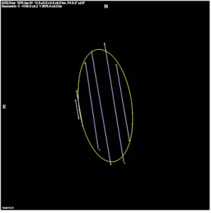
1.9 First ever multi-chord event by an asteroid, according to Oc-cult: (433) Eros, 1975/01/24. Green and red lines represent beginning and end of chords (chords are nearly vertical in this image). Image by Occult. . . 48

1.10 Positive events, per year, according to Occult. Also labelled are some of the main catalogues used for occultation predictions at the year of their release. . . 51

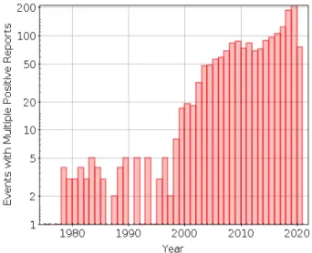
1.11 Number of events with at least one positive occultation, per year, according to Occult. . . 51

1.12 Number of events with at least two positive occultations (al-lowing more accurate astrometry and possibly diameter deter-mination or shape modelling), per year, according to Occult. . 52

1.13 Magnitude Distribution of stars used for reported positive oc-cultations, according to Occult. First column represents stars with V<2 and last represents V>15. Given the typically small telescopes used, there is a bias against fainter stars, as these are far more numerous. Data from Occult. . . 52

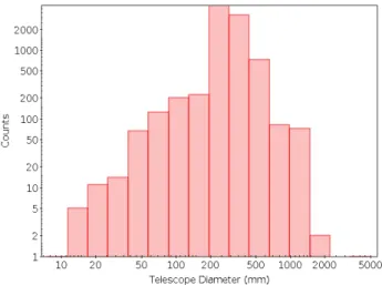
1.14 Reported observations by aperture from 1997 to 2006. Small telescopes (less than 30cm of diameter) are the most used. Im-age by Eric Frappa. . . 53

1.15 Same plot, but cumulative data from 2009 to 2018. Source is also Euraster. . . 53

1.16 (345) Tercidina observed by several dozens of astronomers in September 17th _{2002. Shape becomes much simpler to model}

with multiple observations, as well as the correction of system-atic errors in each individual observation. Image by Euraster. 54

1.17 Occultation by Neptune’s moon, Triton, the first one using DR2 data (Chord 11 was observed in Nice). This event actually pre-dated DR2, with this data being released ahead of time specifically for this occultation. Image by Euraster. . . 55

1.18 Bessel Fundamental Plane. This allows us to use observations made on different sections of Earth’s surface in a single plane, in order to combine those observations’ data. Image by G. Pieper, published in Wikipedia. . . 56

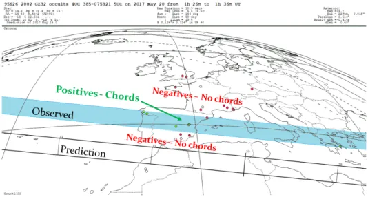
1.19 Correction to the orbit of (95 626) 2002 GZ32, which was made possible due to the several positive and negative reports. Green points are sites with positive reports, and red have negative re-ports. Original image from Steve Preston’s predictions, edited by Jean Lecacheux (LESIA, Paris Observatory). . . 56

1.20 Example of an atmosphere, in this case Triton, visible during the occultation thanks to a central flash. Result obtained by Rui Gonçalves in Constância, Portugal. Similar result obtained in Nice shown in Figure 4.1 . . . 57

1.21 Example of a ring system being detected thanks to stellar oc-cultations, in this case the centaur (10 199) Chariklo. Discovery made in 2014 [Braga-Ribas et al., 2014]. . . 58

1.22 Example of a multiple asteroid system detected via occulta-tions: (87) Sylvia (main body) and its satellites Romulus (far left) and Remus (bottom centre). This observation was a Eu-ropean campaign that included 36 detected chords and 14 neg-ative observations. Sylvia has a radius of 277 km, Romulus 22 km and Remus 11 km, with a separation of several Sylvia radii between them. Image by Euraster. . . 58

1.23 Example of the light of a star changing with time because of an occulting object with an atmosphere and rings. Image by J. L. Elliot [Elliot, 1979] . . . 59

1.24 Gaia satellite (image by ESA). . . 61

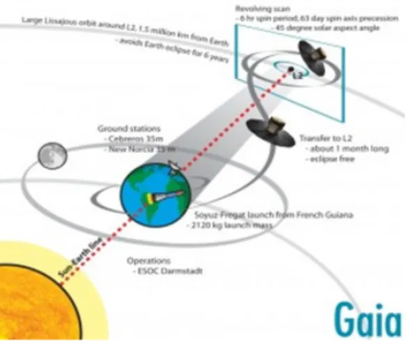
1.25 Trajectory of Gaia from Earth to the L2 point, image courtesy of ESA. . . 62

1.26 Historical progression of astrometry precision until Gaia, with some of the most important catalogues of their time and their size. Image from [Høg, 2011] . . . 64

1.27 Distribution of star Uncertainty (position + proper motion for RA and Dec) with Gaia DR2 for stars of magnitude 14 or below. A random sample of 3 million stars was chosen within the Gaia data. Vast majority has sub-mas uncertainty. . . 64

1.28 Projection of how Gaia will increase precision in orbital uncer-tainties of MBA. This is taken from [Gaia Collaboration et al.,

2018a], where the orange points represent the expected astrom-etry quality from DR2, the black points the current state-of-the-art results from other methods, and the red and blue points represent the expected improvement with 5 and 10 years of Gaia data, respectively. We can see that, for a five-year mission, the state-of-the-art orbital uncertainties can be improved by a fac-tor of up to 10, and since the mission has been extended to 9 years, the 10 year projection is more likely to be the scenario with the final catalogue, bringing an improvement of up to 2 orders of magnitude. These values will be used in Chapter 2 . 66

1.29 DR2 data vs other methods combined for Asteroids. Image by [Gaia Collaboration et al.,2018a]. . . 67

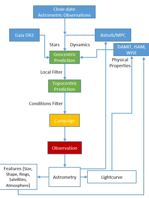
1.30 Schematic of how occultations are prepared and what their con-tributions help with. . . 69

2.1 UniversCity Telescope. Image by Eric Bondoux (OCA). . . 74

2.2 Expected Noise distribution for UniversCity and exposure time of 0.1 s, star at zenith, as function of V magnitude. Line de-scription: black continuous line is the total expected flux, red continuous line scintillation noise, horizontal long dashed green line is the static noise brought by the background, readout and dark current sources, blue short dashed line is photon noise and yellow short dashed line is the total noise, adding the previously mentioned sources. We can see that scintillation dominates for magnitudes smaller than 9 and the static noise dominates starting from magnitude 11. This means that, for fainter stars, improving the available equipment, within reason, to minimize readout and dark current noise should allow a bigger improve-ment than changing the exposure time. . . 76

2.4 SNR Distribution, exposure time of 0.1 s, as function of V mag-nitude. Line description: black, continuous line is the expected SNR at each magnitude step, and the horizontal lines, from highest to lowest, represent SNR of 10, 5, 3 and 1 for compari-son. We can see that for 0.1 s, we reach an SNR of 3 at around magnitude 13, meaning from this point forward detecting the target star should be difficult, and a SNR of 1 just beyond mag-nitude 14, meaning from this point the source is mixed in the background, theoretically remaining undetected. . . 77

2.5 Same as previous figure, but with dt = 0.5 s. Now, SNR of 3 is reached around magnitude 14.5 and SNR of 1 around magni-tude 16, showcasing how much further we can push the target star brightness if a larger exposure time is possible. . . 78

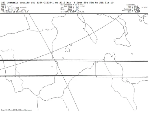
2.6 Path predicted for the Pluto event mentioned in Chapter 1 be-fore DR2 data for the star was available. Central line crosses centre of France, southern limit crosses northern African coun-tries and there is no north limit, as the shadow went all the way to the North Pole. Image by Josselin Desmars, Lucky Star Project. . . 79

2.7 Pluto shadow path once DR2 data for the star was used. Mas-sive shift towards south, with the central line now crossing the northern African countries, the southern limit crossing some central African countries and the northern limit now below the North Pole, excluding a few stations in Nordic territory. Over-all, shift towards South was of over 1 000 km, and while not visible on this image, the uncertainties also decreased massively, giving great confidence to all stations in the new shadow path that they would detect the event. Image by Josselin Desmars, Lucky Star Project. . . 80

2.8 Star Magnitude distribution, with an expected behaviour of more events for fainter stars, which are more numerous. . . 81

2.9 Magnitude Drop distribution, showing that usually the drop is very large, as even a 1 magnitude drop corresponds to a flux shift of approximately 60%. . . 81

2.10 Asteroid Diameter distribution, again with an expected be-haviour, as small asteroids are more frequent than large ones.. 82

2.11 Max Duration distribution, with durations smaller than 1 sec-ond dominating this survey. . . 82

2.12 Star uncertainty from Gaia, with position and proper motion, stars with magnitude 13.5 to 14. Errors below 1 mas clearly dominate. . . 83

2.13 Similar analysis, but magnitudes 11 to 12.5. . . 83

2.14 Asteroid Uncertainty Distribution, in mas, for all events visible from Calern analyzed. . . 84

2.15 Same analysis, also in mas, but for star uncertainty. . . 85

2.16 Star/Asteroid uncertainty ratio for all events. The peak is around 0.1, meaning the star’s uncertainty is 1 order of magni-tude below the asteroid’s, with only a small minority of events having such a poor star precision that it became relevant in the overall event uncertainty. There is, however, a large distribu-tion, meaning we can not always neglect the star’s contribution. 85

2.17 Star/Asteroid uncertainty ratio comparison between UCAC4 and DR2. Only stars that were present in both UCAC4 and DR2 and had a 5-parameter solution in DR2 were included, hence the difference from Figure 2.16. There is an average in-crease of 2 orders of magnitude and, while before, with UCAC4, the star and the asteroid had, on average, comparable uncer-tainties, now the star’s contribution is almost always negligible. 86

2.18 Representation of the effect on an asteroid’s occultation prob-ability as a function of a normalized distance from its centre in units of object diameter, for several uncertainty proportions. A distance of 0 means the site is at the shadow path’s centre, and 0.5 Diameters corresponds to the predicted shadow path limit. 87

2.19 Shift in Magnitude distribution, depending on asteroid orbital quality. We can notice that, the further we decrease the as-teroid’s uncertainty, the more weight we give to long events, filtering out shorter events, which are typically associated with big error margins. . . 89

2.20 Shift in Diameter distribution, depending on asteroid orbital quality. Big diameters become more and more important, not only because of the bigger shadow area they cover, but because these events typically have lower error margins to begin with. 89

2.21 Shift in Event Probability distribution, depending on asteroid orbital quality. As expected, events with low probabilities tend to disappear, either because they became too unlikely in the new run, or because their probability is now much higher. Big-ger efficiency in observations to be expected. . . 90

3.1 DNR distribution for the simulations used, which depends on combined star+asteroid magnitude and the expected magni-tude drop. Since higher DNR imply an easier event to track, we prioritised low DNR combinations of magnitude and drop. 98

3.2 Distribution of Diameter value and uncertainty in WISE sur-vey (122 594 asteroids). Colour plot is the precision, Uncer-tainty/Size, for easier reading. Two main trends exist, of pre-cision 5% and 25%. . . 100

3.3 Discrepancies in Diameter values of IRAS [Ryan and Wood-ward, 2010] and WISE [Masiero et al., 2011] surveys (2 141 common asteroids). In some extreme causes, we can get dis-parities of over 50%, and a difference of 20% or more can be found for ∼20% of the sample. . . 100

3.4 Example of case with high DNR (12.0): Magnitude 11.5, drop 1.0 and 10 points inside occultation.. . . 102

3.5 Example of case with middle-of-the-road DNR (4.9): Magni-tude 12.5, drop of 0.4 and 8 points inside occultation. . . 102

3.6 Example of case with low DNR (2.1): Magnitude 13.5, drop 0.7 and 2 points inside occultation. . . 103

3.7 Prior vs Posterior Distribution of Flux for Intermediate exam-ple. Vertical lines represent medians. . . 103

3.8 Same, but for drop. . . 104

3.9 Same, but for duration. . . 104

3.11 Example of correlation check between Duration and Drop for the "Easy" case.. . . 105

3.12 Same, but between Duration and Centre Epoch. . . 106

3.13 Distribution of the significant (left, green peak) and non-significant (right, blue peak) solutions found by the BIM as a function of the uncertainty on the centre epoch t0, expressed in percentage

of the sampling time. At around 100% uncertainty, the fre-quency of the two situations is about the same. This results are for the Gaussian priors. . . 107

3.14 The figure represents the expected uncertainty resulting from the BIM fit (Gaussian priors) on the duration L (left) and the center epoch t0 of the occultation, as a function of the DNR.

The dots represent each result obtained from a simulated oc-cultation. The continuous black line is the smoothed average value, while the shaded areas enclose the quantiles equivalent to 1-σ and 2-σ. The expected trend ∼ 1/DNR (red dashed line) is visible in both plots. The uncertainty is expressed, re-spectively, as percentage of duration and of sampling time. . . 109

3.15 Distribution of the Bayesian detection probability obtained by the BIM, for the false positives (blue population rising towards the left) and the true events (red population rising towards the right). For the true events the distribution is strongly domi-nated by the peaked around the significance threshold of 99%. For the false positives the detection probability remains always very small. The probability of false positives is ∼ 10−4 _for

significant events. . . 110

3.16 Comparison of the performance on the centre epoch as a func-tion of the DNR, for the Gaussian (blue curve) and Uniform priors (red). Here, only the average value is shown. Despite the relatively small difference, the Gaussian prior has a better performance for more difficult events. . . 111

3.17 Expected distribution of the astrometric uncertainty on the sin-gle chord estimated by our accuracy model, applied to a large set of predictions. Only the component of the uncertainty rel-ative to the fit of each light curve by the BIM is taken into account. The colour corresponds to the chord length, expressed as the number of data points within the light curve minimum. 112

3.18 Uncertainty including the AT error as derived from a simple model (half of the asteroid apparent radius, computed for each event) for a single-chord event, meaning there would be no other observation to this occultation besides ours. For D< 10 km and occultation duration <5 samples, the uncertainty due to aster-oid size no longer dominates and the two error distributions overlap. . . 112

3.19 Tests made with the LSF as a function of whether they were rejected or not vs DNR. Rejected means not fitting the curve, not being able to estimate parameter uncertainties or estimat-ing these uncertainties as beestimat-ing several orders of magnitude above the nominal values. Only 48% of cases were accepted. . 113

3.20 PyOTE’s estimate of the duration of the Daphne occultation. This was the case with the largest DNR among the analyzed (∼7.8). . . 114

3.21 PyOTE’s estimate of the duration of the Victoria occultation. Centre line is best fit, other lines are separated by 1-sigma in flux and duration. This was the case with the lowest DNR among the analyzed (∼1.4). . . 115

3.22 DNR and uncertainty on central epoch for a number of observed events similar to those adopted for the simulation. The colour of the circles is associated to the number of data points in the occultation minimum, indicated by the scale at the right of the plot. Red line represents the average expected uncertainty for the event, and the green areas represent 1 (dark green) and 2 (light green) sigma intervals. Note that the points represent the uncertainty in time obtained through the BIM, NOT the times reported. For the performance comparison between reported uncertainties and the ones obtained through the BIM, check Table 3.2. . . 118

4.1 Triton light curve. Central flash observed, which can be used to study Triton’s atmosphere. . . 122

4.2 Triton occultation analyzed by the Paris team (Bruno Sicardy et. al). Blue line is Neptune’s flux, red line the occulted star’s flux. Black is the ratio between the two, normalised to 1 for the average outside the occultation. . . 123

4.3 Fit of some observed chords of Triton during this event. Our observation is close to the centre. Image by Euraster. An image with all the used chords will be provided in a future publication by the Lucky Star collaboration. . . 124

4.4 Aemilia occultation, seen with AOTA (Asteroidal Occultation Timing Analyzer), a tool present in Occult. The blue dots represent the samples, with their 1-sigma uncertainties, and red lines represent the flux inside and outside the occultation, as well as the slope seen in one and another direction with a 1-sampling time interval. Ingress and egress times in local unites (+2 UTC).. . . 125

4.5 Occultation of (3200) Phaethon as seen with a 1 meter telescope in Nice. Observing team: Jean-Pierre Rivet, Paolo Tanga, Er-ick Bondoux, David Vernet. . . 127

4.6 Shape of (3200) Phaethon fit to the three observed chords: Baba Aissa from Algeria (blue), Christian Weber from Ger-many (red) and our observation (purple). Dashed green and red lines represent uncertainties in disappearance and reappearance moments for each chord, which shows the Nice observation was far more precise than the others. Fit made by Eric Frappa. . . 128

4.7 Millman occultation, as analyzed with Tangra. Blue is the light curve of the occulted star and yellow the light curve of a reference star in the Field Of View. . . 129

4.8 Occultation of (5638) Deikoon, fitted for the 2 positive chords (Lionel Rousselot, Vierzon, France, and Alain Figer, Paris, France). Dashed lines represent timing uncertainties by each user, and their large size does not exclude a spherical model for the asteroid. Our observation is represented by the purple line, numbered 11, meaning that we missed the event by a little over 1 object radius (∼50 km). Fit made by Eric Frappa, shared in Euraster.. . . 133

4.9 European results of (307 261) 2002MS4 campaign. Our obser-vation is the first negative chord to the north. Results will be published by the LESIA team in the future. Image by Euraster.137

4.10 DIAMONDS applied to the OBSPA Europa observation. Re-ported duration was 104.66 ± 1.25 s. Obtained duration with DIAMONDS was 115.9 ± 5.8 s. A difference of 11.3 s that corresponds to a 2-sigma discrepancy. . . 138

4.11 DIAMONDS applied to the FOZ Europa observation. Re-ported duration was 115.52 ± 1.32 s. Obtained duration with DIAMONDS was 114.3 ± 2.4 s. A difference of only 0.8 s, so good agreement between both results. . . 139

4.12 Galatea plot. Red line represents light curve from BIM, while Green lightcurve represents the first approximation found by Rui Gonçalves. Blue points represent the obtained photometry. 140

4.13 Light curve of Euphrosyne. Results reported were duration of 18.56 ± 0.04 s and mid epoch at 00:43:10.30. Results with DIAMONDS were duration of 18.4 ± 0.05 s and mid epoch at 00:43:10.20. Results were compatible within 1-sigma. . . 141

5.1 A single chord occultation is ambiguous. The chord can al-ways fit two different positions for the object, here assumed to be a sphere of Diameter D, usually extracted from WISE. The distance between the observed chord and the two possible solutions can be defined as in Equation 6.1 . . . 148

5.2 Idealised scheme of the uncertainties involved in the astrometry derived from single chord observations of stellar occultations. We adopt as an example a very elongated ellipsoidal asteroid, projected on the fundamental plane in which the asteroid is at rest and the occulted star moves along the dashed arrows. The AC and AT axes represent the across and along–track direc-tions, respectively. In (a) the observed chord duration (black segment) is the same as for the surface-equivalent sphere in (b). The mid-chord point corresponds to the barycentre position in (b), but not in (a), where the error on the derived astrometry eAT cannot be estimated without a precise knowledge of the

shape. Points (c) and (d) represent the ambiguity on the AC position of the observed chord, which can be on opposite sides of the barycentre. . . 149

5.3 There are 4 clear trends, all relating to the rules of AC and AL uncertainty for poor chords, a majority of the archive. Here, we can see that events with 3 or more chords tend to stay out of these trends, as they usually provide good enough astrometry for a particular solution. The rest are distributed across AL being 2, 4 or 8 times smaller, depending on chord length. . . . 151

5.4 Some events with 3 or more chords still fell on the trends, likely due to poor distribution of chords, or poor chord precision, like visual observations or observations with an NTP server with bad synchronization rather than observations timed by a precise system such as GPS. . . 151

5.5 Example of an outlier that fell in the trendline. One of the chords was visual, and therefore left out of the fit, and the other 3 chords were too close to provide a good constraint on the object's position. . . 152

5.6 AL uncertainty in mas as a function of the number of chords of an event. The transition from 2 to 3 chords seems to be when there is a major improvement in the fit, telling us which should be our cutoff on the number of chords for this work. This is to be expected as, with few exceptions, three chords is when an unambiguous fit to the asteroid becomes possible. Since most occultations correlate Along and Across Track uncertainties, a similar plot with Across Track has a similar distribution, with higher uncertainties. . . 152

5.7 Sky-projected distance from both ephemeris to the centre epoch astrometric solution of (51) Nemausa for its 1983/09/11 occul-tation. TS20 clearly approaches the published position, having it almost within a 1-sigma distance. Asteroid had apparent size of 125 mas, putting the FV15 fit outside the body in the AL direction. Both models are compatible in AC direction. . . 156

5.8 Despite the general improvement brought by the TS20, FV15 still usually provides good solutions, with the best case being that of (1 263) Varsavia, an event from 2003/07/08. Asteroid had apparent size of 25 mas, putting the TS20 fit outside the body for the AL direction, though it remains compatible in AC direction. . . 157

5.9 One of the best improvements, that of (212) Medea’s event, on 2011/01/08. Asteroid had apparent size of 92 mas, putting the FV15 fit outside the body. . . 157

5.10 Anomalous (472) Roma event, on 2010/07/08. The star was particularly bright (Vmag. 2.5), with several of the observations having large timing errors, in the order of seconds, likely due to unconventional equipment, such as non-fast moving cameras, being used, or in some cases visual reports instead. Saturation issues may have also played a role on the unreliability of some results. . . 158

5.11 Example of event where TS20 greatly outperformed FV15, an occultation by (41) Daphne on 2012/02/23. . . 162

5.12 Example of event where TS20 greatly outperformed FV15, an occultation by (8 931) Hirokimatsuo on 2017/11/15. . . 163

5.13 Example of event where TS20 greatly outperformed FV15, an occultation by (521) Brixia on 2011/05/27. . . 164

5.14 Correlation between Across and Along Track Differences (in units of diameter) and H0 magnitude of asteroid. There is a positive correlation, suggesting that the differences tend to be larger for larger magnitude asteroids, which correspond to smaller diameters. . . 165

5.15 Same plot, but with Observations available for fit as auxiliary colour. There seems to be a negative correlation, as less obser-vations can bring up the error, which is to be expected. . . 165

5.16 Density distribution of AC distance as a function of asteroid radius vs asteroid size, showing a negative correlation. Red means low density and green/blue high density. . . 166

5.17 Distribution of difference to occultation solution in AC differ-ence, in units of asteroid diameter. Both are centred on 0, and seem to display gaussian behaviour. Gaussian line is for illustration purposes. . . 166

5.18 Similar plot to Figure 5.17, but for differences in AL direction. Once again, gaussian distributions centred in 0, meaning no biases are noticeable. . . 167

5.19 Astrometric solutions of (145) Adeona at the moment of its oc-cultation. The origin of the plot is the position derived from the occultation, in blue. The ellipse is exaggerated, and cor-responds to a 10-sigma region, and the arrow represents the velocity vector. To the left, in orange, is the fit with MPC data only. To the right, in green, the fit with MPC and Gaia combined.168

5.20 Plot similar to Figure 5.19 for (13 244) Dannymeyer, an asteroid with a single chord occultation on November 7th 2019. The

discrepancy between the solutions is larger now, as this asteroid has not been observed as many times as (145) Adeona. . . 168

5.21 Shape solutions obtained with OrbFit for the (50) Virginia oc-cultation. Adding Gaia data improves the agreement between orbital fit and occultation. Chords for MPC+Gaia solution show in green, to better illustrate what was observed. . . 169

5.22 Shape solutions for (145) Adeona occultation. The orbital so-lution does not depend heavily on the Gaia observations, likely due to already good constraints prior to adding them, and so the results are similar. . . 170

5.23 Shape solutions for (163) Erigone occultation. Once again, the orbit is relatively unchanged, with a noticeable deviation in RA from the occultation’s solution. . . 171

5.24 Shape solutions for (118) Peitho occultation. The most drastic change, in favour of adding Gaia data, with the difference going from almost 100 mas to less than 10 mas.. . . 172

5.25 Prediction of occultation by (100) Hekate on March 13th _2020.

The cross represents the site of observation at OCA. Using all MPC observations, but not Gaia, the across axis uncertainty is 37 mas, slightly smaller, but comparable, to the diameter of the object. The probability of a positive detection at our site was calculated at 33%. There were 3 009 observations to this asteroid in total, ranging from 1871 to 2020. . . 173

5.26 113 observations by Gaia to (100) Hekate were added to the orbital fit. This causes a decrease on the across axis from 37 to 3 mas, our site is now inside the shadow path, and the probability raised to 91%. . . 174

5.27 Comparison of semi-major axis uncertainty (in au) for the 14 099 asteroids in DR2 with and without Gaia data. Despite the limited number of observations (a few hundred among thou-sands, on average) and the small time frame of DR2 (22 months vs tens of years with other methods), there is a clear tendency for a drop of σa, with an average drop of ∼17%. . . 174

5.28 Zoomed in version of Figure 5.27, showing us that larger dis-tances result in greater decreases, likely because these objects (Centaurs) have less observations than MBA, giving Gaia a greater weight. . . 175

5.29 Smoothed average of semi-major axis uncertainty as a function of asteroid Diameter. We see that the uncertainty distribution lowers slightly when adding Gaia data across all sizes. For better visualization, TNO were excluded, due to their big size and semi-major axis uncertainty skewing the plot. . . 175

6.1 Example of occultation short term prediction of (65 803) Didy-mos obtained using Occult with the Gaia15.5 catalogue built for this work. . . 183

6.2 Another example, with one of the best NEA in terms of orbital precision, (68 950) 2002 QF15, theoretically visible at Calern. AC uncertainty of 15 mas. . . 183

6.3 Example of event found for (65 803) Didymos in the time frame until the launch of ESA’s HERA spacecraft (2024). AC uncer-tainty of 10 mas. . . 184

A.1 Example from Veres et al. (2017) of dependence of the residuals to the year of observation for a specific site (code 691 -Spacewatch). Different observatories have different trends, so each needs its own rule. This also applies to other parameters. 199

A.2 Same analysis, also from Veres et al. (2017), but with depen-dence on object brightness (code 699 - LONEOS). . . 200

A.3 Same analysis, also from Veres et al. (2017), but with dependence on object projected velocity in the sky (code 699 -LONEOS).. . . 200

A.4 Trend of residuals as a function of catalogue for RA and Dec. "No catalogue" tens to have larger residuals, Gaia DR1 and DR2 smaller, and a large scatter is seen with UCAC catalogues, especially UCAC2. . . 201

A.5 Same analysis, for asteroid magnitude. "No mag" means that no magnitude is given for a certain observation, focusing only on astrometry. Observations that don’t allow a magnitude es-timate tend to be difficult, so these result in larger residuals. Then, there is a clear trend for larger residuals associated to larger magnitudes, similar to what was verified in FV15. . . . 202

B.1 Setup file for mandatory global run of events, readable by Linoc-cult. Dates of run are from 01/01/2018 to 31/12/2018, so one full year. "MinDiameter" is the minimum diameter of an as-teroid, meaning any diameter smaller excludes the object from this run. "MaxDiameter" does the same with an upper bound, but is left unused. Results are output in a .bin file which will then be used to extract local events.. . . 207

B.2 User sites file, that Linoccult reads together with the .bin global file to assess events visible in specific locations.. . . 207

B.3 Local Linoccult file. "SitesFilePath" indicates where Linoccult must read the site file, "InputEventsFilePath" where to read the .bin file and "Calculation Mode 0" ensures Linoccult does not compute globally every event again, just for the local sites. 209

B.4 Setting up all relevant variables for the simulation. . . 209

B.5 Flux calculation for specific event. . . 210

B.6 Getting every star within a certain Declination band that fol-lows all of our restrictions. . . 211

B.7 Section in Occult which builds the Gaia star catalogue from our output files. . . 212

B.8 Getting every observation from a specific asteroid made by Gaia. This example shows the query for the lowest numbered asteroid in the catalogue, (8) Flora. . . 213

B.9 File that queries AstDyS for the initial values of orbital pa-rameters of every asteroid in DR2, whose MPC numbers are extracted from a source file made previously. . . 213

B.10 File that queries MPC for all available observations of each asteroid present in DR2. . . 214

B.11 Example of a setup file to be read by OrbFit, in this case for (1 566) Icarus. Main difference between runs is whether the error model used for the observations is the previously established one (Farnocchia - fcct14) or the new one built by Federica Spoto (gaiaDR2).. . . 214

B.12 Example of application of photutils to a stellar occultation. Target was Pluto, for an occultation on 2016/07/14 in Con-stância. By using a FITS file for each frame (1024 x 1024 pix-els), photutils analyzes searches for sources above noise level by a certain threshold (signal 5x larger than noise in this ex-ample). Then, it lists the (x;y) pixel coordinates of each target that surpasses this threshold, and by using a first approach, we attempt to manually identify in the first frame which of these targets is the occulted star, doing aperture photometry of 3.5 pixels radius around it, the value found to have the best SNR for targets that are not very bright. Other stars, should they be above the threshold for the entire video, can be used as reference later. Once the occulted star has been found, we search its surroundings in the following frame for it. If it is not found, then we assume it remains in the same coordinates, which should be the case for stable images. This is necessary in case the drop caused by the occultation is large enough to remove the star from the list of objects above the threshold. A different approach is to use relative positions by taking a few reference stars, and using their positions to estimate the position of the lost target. . . 215

1.1 Average precision in star precision for different magnitudes in DR2. G < 15 is the most relevant group for this work. . . 65

1.2 Stars with 2 or 5 parameter analysis in each DR, as well as number of objects with an estimated G magnitude. Number of objects with 5-parameter analysis grew by 3 orders of mag-nitude between DR1 and DR2. Such jumps will not be seen in DR3 or any future releases for the stars, but there is still a growth of events with good star astrometry to be expected with the newer catalogue, and a lot more asteroids in DR3 and beyond, this new version representing for Solar System Objects what DR2 was for the stars. . . 68

2.1 Expected efficiency for specific site, depending on asteroid un-certainty improvement. . . 88

2.2 Table listing, for each asteroid uncertainty improvement factor and for each asteroid size category, how many events have prob-abilities above 1% (minimum for observation planning), 25%, 50% and 75%. Clear trend of less unreliable events is found, as should be expected. . . 91

3.1 Performance comparison between PyOTE and DIAMONDS, the two bayesian tools available. Centre epoch precision is shown to be of comparable size most of the time, with DIA-MONDS benefiting from being more versatile in the choices made and more user friendly for mass use. . . 116

3.2 Observed occultation chords chosen for comparison to our model for observation accuracy. Their photometric light curves data have been fitted by the model, with the same procedure adopted for the simulations. For the (3 200) Phaethon observation in particular, since our uncertainty was the one published, the "author" uncertainty is the one obtained by Jean-Pierre Rivet, another member of the observation, through a different method. For the other observations, the uncertainties were obtained from various sources, namely the Planoccult mailing list where the observers shared their reports, Euraster and the Occult archive. σt0 R is the reported uncertainty, σt0 B (s) the

uncer-tainty obtained with the BIM and dt the exposure time. . . . 117

5.1 Rule applied by [Vereš et al.,2017] to the epoch of each asteroid observation. . . 146

5.2 Rule applied by [Vereš et al., 2017] to the method of each as-teroid observation. . . 147

5.3 Rule applied by [Vereš et al., 2017] to the reference star cata-logue of each asteroid observation, for RA and Dec coordinates separately. . . 147

5.4 Table of every asteroid occultation with 20 or more positive chords reported, sorted by ascending asteroid number. Dis-tance to astrometric solution of occultation by FV15 and TS20 error models are shown, with a clear trend of better solutions under TS20. . . 155

5.5 Comparison between the error models FV15 and TS20 by us-ing OrbFit. We analyze average and σ of AC, AL and total differences. We can see that using the current database for each asteroid provides better results, as is to be expected, as more modern observations tend to be more precise. We also see a tendency for differences to become smaller by adopting the TS20 model rather than FV15. . . 159

5.6 Same as Table 5.5, but as ratio of difference and apparent diam-eter at moment of occultation, along with percentage of events that fell within one diameter of difference to the occultation. This percentage means how many events would have been con-firmed by the occultations, barring issues regarding irregular shapes or bad chord distribution. Like in Table 5.5, current knowledge improves results compared to "postdictions" and TS20 outperforms FV15. . . 160

5.7 Same as Table 5.5, but only for events with 5 or more chords, which are typically the most precise. About 8% of events (∼370) fall under this category. Results tend to be slightly further away on average, but the progression by using current knowledge vs "postidction" and TS20 vs FV15 is still present. 160

5.8 Same as Table 5.6, but only for events with 5 or more chords. 160

5.9 Determining which model is better or whether they are similar. Here, we adopt the convention that they are similar if their distances to the occultation’s astrometric solution are within 10% of the larger distance. If not, then whichever model is the closest is considered to be better. We can see that, for the non-similar results, TS20 was better more than twice the amount of cases than FV15. . . 161

5.10 Distribution of events in different regions of AC difference: "d < R", where the difference is smaller than the asteroid’s radius, "1-sigma", where the difference is between R and R + σocc +

σmodel, "3-sigma", where difference is between R + σocc+ σmodel

and R + 3 ∗ (σocc + σmodel) and "incompatibility", where the

difference is even larger. We also separate the data set between stars with known issues from DR2 that the rest, showing that, if these issues were to be treated, results would improve. Only the runs with the best current knowledge were used for this analysis, and once again TS20 outperforms FV15. . . 161

6.1 All 11 NEA with σa < 10−9 au, in ascending order. Full list

of "interesting" targets included the 70 best NEA in terms or semi-major axis uncertainty, plus (65 803) Didymos for the HERA mission. . . 184

Introduction

Contents

1.1 Asteroids History . . . 37

1.1.1 How have they been observed? . . . 37

1.1.2 Observation Methods and Missions . . . 43

1.2 Stellar Occultations . . . 45

1.2.1 General properties . . . 45

1.2.2 Why are they important? . . . 54

1.3 The Gaia Mission . . . 60

1.4 Goals and Structure of this Thesis . . . 68

1.1

Asteroids History

1.1.1

How have they been observed?

Asteroids are small bodies of our Solar System that have been known since the early 19th _{century. The very first one to be discovered is also the biggest}

known object of the Main Belt, (1) Ceres (Figure 1.1), with a diameter of 945 km, discovered in 1801 by Italian astronomer Giuseppe Piazzi.

Its existence was hinted at by an empirical law derived by Johann Elert Bode in the 18th _{century, who, through a geometric distribution of the known}

planets at the time (Mercury to Saturn), stated that there should be a planet between Mars and Jupiter. However, in the following decades more objects were discovered in this region, such as (2) Pallas, (3) Juno, (4) Vesta and (5) Astraea, until in 1846 the discovery of Neptune rendered this Law discredited.

Figure 1.1: (1) Ceres, the first asteroid discovered and largest object of the Main Belt. Image by NASA. Image from Baer et al. [2011]

Astronomers kept looking for new objects between Mars and Jupiter, as well as beyond Neptune, reaching 1 000 numbered asteroids in the 20s, 10 000 in 1989, 100 000 in 2005 [Tichá et al., 2007] and over 540 000 nowadays, to which we can add another 450 000 unnumbered asteroids [DeMeo et al.,2015]. The recent evolution of numbered asteroids, as well as Near Earth Asteroids in particular, can be found in Figures 1.3 and 1.4.

The known population of asteroids can be considered to be known with reasonable completeness down to diameters of 5 km, with smaller sizes be-ing under-represented due to the biases imposed by the observation methods, which usually favour larger and/or brighter objects. You can see the distri-bution in Figure 1.2

Asteroids are important because they are the remnants of the formation period of our Solar System’s formation. Their composition and distribution allows us to peek into those early days, and study how our system evolved from then until now. Another useful reason to study them is for our own defense, since we are constantly being bombarded with small objects, and on occasion large bodies hit the Earth, which may cause permanent changes to our landscape and considerable losses. Studying asteroids can help prevent

Figure 1.2: Diameter distribution of numbered asteroids, according to the NEOWISE survey. Diameters smaller than 5km are assumed to be heavily under-represented due to the biases introduced by the limitations of the most typical observation methods.

this from happening in our future. Finally, nearby asteroids may also be in-teresting to study as an exploitable resource, depending on their composition, though for now missions to asteroids remain very costly.

Nowadays, the small bodies of the Solar System are split into different categories, depending on their semi-major axis, composition and interaction with other objects. Some examples are listed.

• MBA: Main Belt Asteroids, objects whose semi-major axis is between Mars (1.5 au) and Jupiter (5.2 au), being by far the largest known sub-group of asteroids;

• TNO: TransNeptunian Objects, objects whose semi-major axis is bigger than Neptune’s (>30 Astronomical Units, au), with Pluto being the most well-known example;

• NEA: Near-Earth Asteroids (also known as NEO - Near Earth Objects), whose closest approach to the Sun (perihelion) is smaller than 1.3 au;

• Centaurs: Semi-major axis between Jupiter (5.2 au) and Neptune (30 au);

• Trojans: Asteroids that share an orbit with a planet, usually Jupiter. These asteroids are in one of the Lagrange points of the Sun-planet system;

• Amor: NEA whose perihelion is larger than Earth’s aphelion, named after (1 221) Amor;

• Apollo: NEA whose perihelion is smaller than Earth’s aphelion, named after (1 862) Apollo;

• Aten: NEA whose semi-major axis is smaller than 1 au, named after (2 062) Aten;

• Atira: NEA whose aphelion is smaller than Earth’s perihelion, named after (163 693) Atira;

• PHA: Potentially Hazardous Asteroids, whose orbits make close ap-proaches to Earth and represent a risk of impact.

Throughout the decades, the method of detecting asteroids has changed. While at first astronomers had to compare plates with sky images to look for objects with noticeable movements nowadays, this process is computer-ized, and accepted sets of observations allow astronomers to estimate orbital parameters and include a new object in the catalogues.

The current preliminary designation method for new objects follows a stan-dard, enumerated.

1. The year of discovery of the object;

2. A first letter ranging A-Y representing the half-month in which the object was discovered within that year (letter I is not used);

3. A second letter ranging A-Z representing the order of discovery within that half-month;

The asteroid gets a permanent catalogue number once its orbit is accurate enough to predict its position at the next opposition with a precision sufficient for its recovery (typically a few arcminutes).

Later, an object’s name can be changed to reference a person, group, place or historical figure, as long as its catalogue number remains the same.

We stress here that, for occultations, we will only be referring to numbered asteroids, as good orbits are usually required for reliable predictions.

Figure 1.3: Number of known asteroids by year in the last 2 decades. Image from Minor Planet Center.

Asteroids are thought to be, along with comets, primordial objects of the Solar System, retaining properties from the planetesimal stage, making their study vital to study the origins of our system. The most complete databases as of right now are Astorb1_{, MPC}2_{(Minor Planet Center),}

AstDyS-23_{(Asteroids Dynamic Site) and JPL Horizons}4_{(Jet Propulsion Lab). While}

all four are used, there are differences between them: MPC is the official database of the International Astronomical Union, and is the group in charge of the provisional and definitive identifiers of small bodies. It updates its observations archive monthly, and details epoch, observatory, method and RA/Dec coordinates for each asteroid observation. Meanwhile, the other 3

1 ftp://ftp.lowell.edu/pub/elgb/ 2 https://minorplanetcenter.net/iau/MPCORB.html 3_{http://hamilton.dm.unipi.it/astdys/} 4_{https://ssd.jpl.nasa.gov/horizons.cgi}

Figure 1.4: Amount of known NEA by year in the last 4 decades. From the scarce growth, it is considered that the population of NEA larger than 1 km is well-known and almost completely catalogued, but the smaller sizes are still under-represented. Image from Minor Planet Center.

Figure 1.5: Mass distribution of the Main Belt, with the pie chart sections in the same order of the legend, in clockwise direction.

sources use the MPC database of observations, but apply their own data selection rules to refine the orbits by rejecting some of the least precise data points (see AppendixA for the rules applied to Astorb and JPL).

1.1.2

Observation Methods and Missions

While this work focuses on stellar occultations and the Gaia space mission, there are several other methods that have been historically used to obtain the astrometry of asteroids, with varying degrees of availability and precision. The following is a list of the most commonly used methods, with the aver-age accuracy taken from [Desmars et al., 2015], and some current or future missions that apply to each category:

• Radar observations: mostly used for close targets, to assess their shape. The rapid decay of the photon flux in this regime makes it so the current set of radar observations is heavily biased towards NEA. It allows to study the size, shape and spin of each body, and can reach kilometer-sized precision in the measurements;

• Thermal radiometry: observations in the micrometer range, to measure the thermal flux of an asteroid. One of the most reliable methods to estimate an asteroid’s size and its geometric albedo.

• Ground-based direct imaging through the use of photographic plates or CCD, which allows relative astrometry, using reference objects around the asteroid to determine its position and apparent velocity, and pho-tometry, the measurement of the flux of the asteroid, helping build shape models. At the time of the paper reference, these accounted for almost 95% of all observations, almost entirely due to CCD imaging in the most recent decades. The average astrometric precision of this method is 300 mas. It should be noted that photometry is one of the methods that allows the build of shape models;

• Space observations, carried out by probes outside of Earth’s atmosphere. This is useful to increase the quality of the image, as it is no longer necessary to account for distortions caused to the light signal by the air molecules. Due to the expensive nature of space missions, this is

not as frequent as ground-based observations, but several space probes, mentioned later in this chapter, have been used for this purpose, with an especially sizeable contribution by the WISE telescope, accounting for ∼4% of all observations. The average astrometric precision from this method is 600 mas. Some highlights for this method are:

– Gaia, analyzed in detail in Section 1.3;

– NEOWISE5 [Masiero et al., 2011], NASA mission. All-sky

sur-vey that discovered thousands of asteroids and provided the most complete asteroid diameter table to date, with over 120 000 mea-surements, and is currently focusing on NEA;

– Euclid6, future ESA mission. Despite focusing on topics such as

the expansion of the universe and the identity of dark matter, it is also expected to greatly increase the available information on spectral classification of asteroids. See [Carry, 2018];

• "In-situ" observations, when space probes target a specific asteroid ei-ther to study it at he surface, or to return samples to Earth. Some examples of such missions are:

– Hayabusa7 [Kawaguchi et al., 2008] and Hayabusa28 [Tsuda et al.,

2013], a completed and an on-going JAXA missions (Japan). Hayabusa landed on (25143) Itokawa, recovered samples from it, and re-turned to Earth, being the first of this kind of missions to return. Hayabusa2 had a similar task to study (162173) Ryugu, and is expected to return in December 2020;

– OSIRIS-REx9 [Lauretta,2015]: On-going NASA mission. Orbiting

the asteroid (101 955) Bennu, and with the goal of return samples from this object to Earth;

– Lucy10: Future NASA mission. Planned to cross several trojan

asteroids, most notably (11 351) Leucus [Buie et al.,2018];

5 https://www.nasa.gov/mission_pages/neowise/mainindex.html 6 https://sci.esa.int/web/euclid 7 http://www.isas.jaxa.jp/en/missions/spacecraft/past/hayabusa.html 8 http://www.hayabusa2.jaxa.jp/en/ 9_{https://www.nasa.gov/osiris-rex/} 10_{https://www.nasa.gov/content/goddard/lucy-overview}

– DART (Double Asteroid Redirection Test)11 [Cheng et al., 2018]: Future NASA mission. Planetary defense test on the binary system of (65803) Didymos. By directly crashing a satellite into the moon of Didymos, which is only 160 m in size, scientists will be able to study the shift caused on its orbit. This is connected to HERA12

[Sears et al., 2004], an ESA mission, that will help measure the consequences of the DART’s impact;

– DESTINY+13 [Sarli et al., 2018]: Future JAXA mission, planned to flyby (3200) Phaethon, to understand the origin of its meteor shower;

– Psyche14 _{[Maurel et al., 2020]: Future NASA mission, designed to}

orbit its namesake, (16) Psyche, and study its composition. Finally, stellar occultations, explained in detail in the next section.

1.2

Stellar Occultations

1.2.1

General properties

A stellar occultation is an event in which a certain object crosses the trajectory of a star’s light from the observer’s perspective. Because of the apparent size of stars and asteroids, this event can only be visible in certain "shadow" areas that the asteroid produces on the planet’s surface when passing in front of a star. The smaller the object, the smaller the size of this shadowed region is, making the event much more difficult to observe, and needing great precision on the position of both star and asteroid better than arc-second size. For that reason, it was not feasible to observe stellar occultations of small bodies for a long time, because their orbits were not precise enough and because until recently even the star catalogues had uncertainties too large to make mass predictions, only applying this method to the Moon and the planets, not only because of their bigger angular size, but because we know their orbits with

11 https://www.nasa.gov/planetarydefense/dart 12 https://www.esa.int/Safety_Security/Hera 13_{https://destiny.isas.jaxa.jp/} 14_{https://www.jpl.nasa.gov/missions/psyche/}