Search for magnetic fields in particle-accelerating colliding-wind binaries

arXiv:1412.5327v1 [astro-ph.SR] 17 Dec 2014

December 18, 2014

Search for magnetic fields in particle-accelerating colliding-wind

binaries

⋆

C. Neiner

, J. Grunhut

, B. Leroy

, M. De Becker

, and G. Rauw

1 _{LESIA, Observatoire de Paris, CNRS UMR 8109, UPMC, Université Paris Diderot, 5 place Jules Janssen, 92190 Meudon, France;}

e-mail: coralie.neiner@obspm.fr

2 _{European Southern Observatory (ESO), Karl-Schwarzschild-Str. 2, 85748, Garching, Germany}

3 _{Department of Astrophysics, Geophysics and Oceanography, University of Liège, 17 Allée du 6 Août, B5c, 4000, Sart Tilman,}

Belgium

Received ...; accepted ...

ABSTRACT

Context.Some colliding-wind massive binaries, called particle-accelerating colliding-wind binaries (PACWB), exhibit synchrotron radio emission, which is assumed to be generated by a stellar magnetic field. However, no measurement of magnetic fields in these stars has ever been performed.

Aims.We aim at quantifying the possible stellar magnetic fields present in PACWB to provide constraints for models.

Methods. We gathered 21 high-resolution spectropolarimetric observations of 9 PACWB available in the ESPaDOnS, Narval and HarpsPol archives. We analysed these observations with the Least Squares Deconvolution method. We separated the binary spectral components when possible.

Results.No magnetic signature is detected in any of the 9 PACWB stars and all longitudinal field measurements are compatible with 0 G. We derived the upper field strength of a possible field that could have remained hidden in the noise of the data. While the data are not very constraining for some stars, for several stars we could derive an upper limit of the polar field strength of the order of 200 G.

Conclusions. We can therefore exclude the presence of strong or moderate stellar magnetic fields in PACWB, typical of the ones present in magnetic massive stars. Weak magnetic fields could however be present in these objects. These observational results provide the first quantitative constraints for future models of PACWB.

Key words. stars: magnetic fields - stars: early-type - binaries: spectroscopic - stars: individual: HD 36486, HD 37468, HD 47839, HD 93250, HD 151804, HD 152408, HD 164794, HD 167971, HD 190918

1. Introduction

Colliding-wind massive binaries (CWB) are binary systems composed of two stars of O, early-B or WR type. Their main feature is a wind-wind interaction region where the shocked gas is very hot (107 _{K). This wind interaction region is likely} to contribute to the thermal radio emission, in addition to the free-free radiation due to thermal electrons in single star winds (Dougherty et al. 2003).

In addition to this thermal emission, non-thermal radio emission was discovered in some systems. It is related to the synchrotron radiation due to the presence of relativistic elec-trons (Pittard et al. 2006). These synchrotron emitters are called particle-accelerating colliding-wind binaries (PACWB). In addi-tion to the synchrotron emission, these systems can be revealed by exceptionally large radio fluxes, a spectral index significantly lower than the thermal value, and an orbital modulation of the

ra-Send offprint requests to: C. Neiner

⋆ _{Based on archival observations obtained at the Telescope Bernard} Lyot (USR5026) operated by the Observatoire Midi-Pyrénées, Univer-sité de Toulouse (Paul Sabatier), Centre National de la Recherche Sci-entifique (CNRS) of France, at the Canada-France-Hawaii Telescope (CFHT) operated by the National Research Council of Canada, the In-stitut National des Sciences de l’Univers of the CNRS of France, and the University of Hawaii, and at the European Southern Observatory (ESO), Chile.

dio flux. De Becker & Raucq (2013) recently provided the most up-to-date catalog of such systems.

High angular resolution observations of some PACWB have allowed to disentangle the thermal and non-thermal emissions (e.g. OB2 #5, Dzib et al. 2013) and showed that the synchrotron emission is associated to the wind-wind interaction region. This region is also a source of thermal X-rays, in addition to the in-trinsic X-ray emission produced in the stellar winds of the indi-vidual components. The X-ray spectrum produced in the wind interaction region is generally significantly harder than that of massive single stars, and the X-ray emission is variable with the orbital phase (e.g. De Becker et al. 2011; Cazorla et al. 2014).

Finally, it was discovered more recently that PACWB may also emit γ rays through inverse Compton scattering by the rela-tivistic electrons and neutral pion decay. However, only one such example is known as of today (η Car, Farnier et al. 2011).

These many characteristics make PACWB very interesting objects to study extreme physical processes. However, it has be-come more and more clear over the last few years that PACWB cover a very wide range of parameters (mass loss, wind veloc-ity, orbital period...) and the fundamental difference between the PACWB and “normal” CWB is unknown (De Becker & Raucq 2013).

The presence of synchrotron emission in PACWB immedi-ately points towards the presence of a magnetic field. Indeed,

synchrotron emission results from the modified movement of relativistic electrons in a magnetic field. Moreover, the accelera-tion of particles in PACWB could be explained either by strong shocks in the colliding winds (e.g. Pittard et al. 2006) or by mag-netic reconnection or annihilation (e.g. Jardine et al. 1996). It has thus been speculated that the fundamental difference be-tween CWB and PACWB is the presence of a magnetic field.

Over the last two decades magnetic fields have been detected in ∼7% of single massive stars (Wade et al. 2014b). While the fraction of PACWB among CWB is not known and the cata-log by De Becker & Raucq (2013) certainly underestimates the number of PACWB, ∼7% could be a plausible proportion con-sidering that only 43 possible PACWB have been identified as of today (De Becker & Raucq 2013) while most massive stars are probably in binaries (Sana et al. 2012, 2014). Therefore, the presence of a magnetic field might indeed be the difference be-tween PACWB and “normal” CWB.

The magnetic field in PACWB could be of stellar origin or it could also possibly be generated in the colliding winds them-selves. From synchrotron observations, one can estimate the magnetic field strength in the wind-wind interaction region to be of the order of a few mG (see e.g. Dougherty et al. 2003). Ex-trapolating to the surface of the stars with typical distances be-tween the stagnation point and the photosphere, we obtain val-ues of the stellar magnetic field strength between one G and a few thousands G, depending on the system and on the assump-tions (e.g. Parkin et al. 2014). Magnetic fields detected in single massive stars have a polar field strength between hundred and several thousands G (see e.g. Petit et al. 2013), which are com-patible with the fields speculated in PACWB models.

Therefore, measuring magnetic fields in PACWB is an ideal way to test these assumptions, constrain models of colliding winds, and understand the difference between PACWB and “nor-mal” CWB.

2. Archival spectropolarimetric observations

An updated census of 43 PACWB has been published recently (De Becker & Raucq 2013). It includes clear PACWB detected through their synchrotron emission as well as candidates from indirect indicators (e.g. radio flux).

We have gathered all high-resolution spectropolarimetric data of these PACWB available in archives, i.e. observed with Narval at Télescope Bernard Lyot (TBL) in France, ESPaDOnS at the Canada-France-Hawaii telescope (CFHT) in Hawaii, or HarpsPol at ESO in Chile. Circular polarisation data are avail-able for 9 of the 43 known PACWB. When several consecutive spectra were available for the same night, we averaged them. The 9 stars and 21 (average) observations are listed in Table 1.

For each star, we normalized the data to the intensity con-tinuum level and extracted Stokes V and Null (N) polarisation spectra. N spectra allow us to check that the magnetic measure-ments (in the Stokes V spectra) have not been polluted by spuri-ous signal, e.g. due to instrumental polarisation.

We then proceeded to use the Least Squares Deconvolution (LSD) technique (Donati et al. 1997) to search for weak Zeeman signatures in the mean Stokes V profile. The input LSD masks for each star were extracted from line lists provided by VALD (Piskunov et al. 1995; Kupka et al. 1999) according to the spec-tral type of each target. These line lists orginally contain all lines with predicted line depths greater than 1%, assuming solar abun-dances. We proceeded to remove all hydrogen lines, lines that were blended with H lines, and lines that are strongly contam-inated by telluric regions. We then automatically adjusted the

Table 1. List of 21 archival spectropolarimetric observations of 9

PACWB, including the instrument used for the observations, date of ob-servations and signal-to-noise ratio (SNR) in the Stokes I and V spectra.

Star Instrument Date SNR I SNR V

HD 36486 Narval 23.10.2008 5386 21947 Narval 24.10.2008 6021 108758 HD 37468 ESPaDOnS 17.10.2008 3149 56388 HD 47839 Narval 10.12.2006 4416 19648 Narval 15.12.2006 4528 37218 Narval 09.09.2007 4497 25269 Narval 10.09.2007 4384 33820 Narval 11.09.2007 4280 24183 Narval 20.10.2007 4545 39090 Narval 23.10.2007 4563 41668 ESPaDOnS 02.02.2012 4863 51425 HD 93250 HarpsPol 17.02.2013 4169 9523 HD 151804 HarpsPol 26.05.2011 6191 22047 HD 152408 ESPaDOnS 05.07.2012 843 12909 HD 164794 ESPaDOnS 19.06.2005 3083 14933 ESPaDOnS 20.06.2005 3298 15249 ESPaDOnS 23.06.2005 3118 15657 HarpsPol 25.05.2011 5050 14081 ESPaDOnS 14.06.2011 3346 29046 HD 167971 ESPaDOnS 30.06.2013 2671 22295 HD 190918 ESPaDOnS 25.07.2010 4096 13892

line depths of each remaining line to provide the best fit to the observed Stokes I spectra.

Using these final line masks, a mean wavelength of 5000 Å and a mean Landé factor of 1.2, we extracted LSD Stokes I and

V profiles for each spectropolarimetric measurements. We also

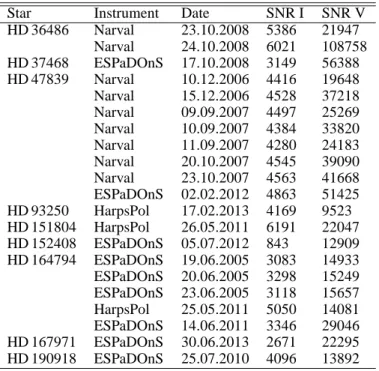
extracted LSD N polarisation profiles to check for spurious sig-natures. All LSD N profiles are flat, showing that the LSD V measurements do reflect the stellar magnetic field. The LSD I and Stokes V profiles of the 9 stars are shown in Fig. 1. LSD V profiles are also flat, showing no sign of a magnetic signature in any of the 9 PACWB.

3. LSD

I

To go further and evaluate the magnetic field in the studied PACWB, since PACWB are binary stars, we first needed to sep-arate the individual spectra of each component in the LSD I pro-files.

For each spectrum we fit the mean LSD Stokes I profile to determine the radial velocity Vrad, the projected rotational broad-ening (v sin i) and any contribution from non-rotational broaden-ing that we consider to be macroturbulent broadenbroaden-ing (Vmac).

Ideally, fits to the observed profiles should be computed with Fourier techniques (e.g. Gray 2005; Simón-Díaz & Herrero 2014) directly on the intensity profiles (rather than the LSD pro-files). However, this is very time consuming and not necessary here since the exact value of the parameters are not important for our purpose. We only need a good fit to the LSD profiles. Therefore, the profiles are computed as the convolution of a rotationally-broadened profile and a radial-tangential broadened profile following the parametrisation of Gray (2005), assuming equal contributions from the radial and tangential (RT) com-ponent. While this form of macroturbulence is not commonly used in the study of early-type stars (typically a Gaussian pro-file is used to characterise Vmac), Simón-Díaz & Herrero (2014)

0

1

V

0.98

1

I

-2

0

2

V

0.98

1

I

0

2

V

0.99

1

I

-2

0

2

V

0.98

1

I

0

2

V

0.98

1

I

0

2

V

-200

0

200

0.98

1

I

-1

0

1

V

0.98

1

I

0

2

4

6

8

V

-300

0

300

Velocity (km s

)

0.98

1

1.02

1.04

I

0

2

4

5

6

7

V

-200

0

200

0.98

1

1.02

1.04

1.06

I

HD37468

HD93250

HD151804

HD152408

HD167971

HD190918

HD36486

HD164794

HD47839

Fig. 1. LSD I (bottom panels) and Stokes V (top panels, y-axis multiplied by 10000) profiles of the 9 PACWB available in spectropolarimetric

archives. When only one spectrum is available (left panels), observations are indicated in black and the fit in red. If several components are present the fit of the primary/secondary/tertiary component is shown in blue/green/pink, while the combined fit is in red. When several spectra are available for one star (middle and right panels), observations are indicated with various colours, and the fits are indicated in black with primary and secondary component fits indicated in green and blue respectively. In these cases, profiles are artificially shifted upwards to ease the reading.

Table 2. Parameters derived from the fit of LSD I profiles of each star.

When several components are visible in the spectra, each component (primary, secondary and possibly tertiary) is fitted. The last column in-dicates the upper dipolar field strength limit in G for each spectrum.

Star Date Comp. Vrad vsin i Vmac Bpol,max

HD km s−1 _{km s}−1 _{km s}−1 _G 36486 23.10.08 97 126 101 206 24.10.08 -4 116 126 906 37468 17.10.08 prim 33 115 124 258 sec 10 28 29 513 47839 10.12.06 prim 32 52 90 867 sec 79 140 154 8579 15.12.06 prim 32 52 90 472 sec 79 140 154 4979 09.09.07 prim 32 52 90 687 sec 79 140 154 5581 10.09.07 prim 32 52 90 543 sec 79 140 154 4104 11.09.07 prim 32 52 90 789 sec 79 140 154 5658 20.10.07 prim 32 52 90 449 sec 79 140 154 3797 23.10.07 prim 32 52 90 428 sec 79 140 154 3837 02.02.12 prim 32 52 90 337 sec 79 140 154 3637 93250 17.02.13 -1.5 92 189 4367 151804 26.05.11 -58 79 83 850 152408 05.07.12 -91 69 154 1363 164794 19.06.05 12 76 180 1600 20.06.05 10.5 75 191 1671 23.06.05 9.5 71 191 1572 25.05.11 8.9 71 186 1765 14.06.11 6.7 69 189 865 167971 30.06.13 prim 13 63 73 1092 sec -16 146 62 1160 ter -212 52 36 -190918 25.07.10 -25 102 111 1960

Table 3. Measured longitudinal field Bland Null polarization Nl, with

their error bars σ. When several components are visible in the spectra, the values were estimated for each component (primary, secondary and possibly tertiary).

Star Date Comp. Bl Nl σ

HD G G G 36486 23.10.08 43 13 38 24.10.08 18 1 7 37468 17.10.08 prim -3 35 19 sec 16 -18 9 47839 10.12.06 prim -27 17 25 sec -260 -173 210 15.12.06 prim -6 14 13 sec 5 256 185 09.09.07 prim 3 -13 20 sec -243 -173 210 10.09.07 prim 8 7 15 sec -41 278 154 11.09.07 prim 14 -14 23 sec -141 -95 211 20.10.07 prim -9 4 13 sec -98 146 140 23.10.07 prim -1 23 12 sec -27 -154 142 02.02.12 prim -6 -4 10 sec 17 22 132 93250 17.02.13 -24 175 135 151804 26.05.11 -13 -34 33 152408 05.07.12 2 60 34 164794 19.06.05 -3 -18 52 20.06.05 -2 44 52 23.06.05 64 25 50 25.05.11 6 87 54 14.06.11 61 29 27 167971 30.06.13 prim 3 -16 40 sec 98 16 59 ter -19 -216 115 190918 25.07.10 8 93 70

showed that it provides a good agreement with the Fourier tech-niques.

The code uses the mpfit library (Moré 1978; Markwardt 2009) to find the best fit solution. Using a radial-tangential pro-file for Vmac tends to maximise v sin i. Therefore the values we obtain for v sin i can be considered as upper limits.

For profiles that show obvious signs of spectroscopic com-panions (HD 37468, HD 47839 and HD 167971) we simultane-ously fit multiple profiles, one for each component, to determine the overall best solution for the given SB2 (or SB3) profile. For HD 47839, since the various spectra show no significant varia-tions, the averaged profile was fitted. The simultaneous fitting of multiple profiles for one spectrum is a difficult task and the so-lution is often degenerate. We therefore attempted to constrain each fit based on previous studies published in the literature whenever possible. For the other stars (SB1), only one compo-nent was fitted.

The various components and the resulting parameters are listed in Table 2. These parameters are only calculated to de-rive upper limits on the magnetic field strength. They should be used with care for other studies as they do not necessarily have a physical meaning. By running the fits several times with differ-ent initial guess values, and by visually comparing the quality of

the fit when changing the parameters, we estimate that the un-certainty on v sin i and Vmac is of the order of 10 km s−1. The uncertainty on Vrad is of the order of a few km s−1. The fits of each individual component, as well as the combined fit of all components, are shown in Fig. 1.

4. Magnetic field measurements

4.1. Longitudinal field measurement

From the LSD profiles we computed the longitudinal magnetic field (Bl) value and the corresponding null measurement Nl

and their error bars σ, using the first-order moment method of Rees & Semel (1979) using the form given in Wade et al. (2000). We applied this measurement to the individual components of each stars, when visible.

The results are reported in Table 3. We find that the Bland

Nlvalues are all compatible with 0 within 3σ. This confirms that

no field is detected in any of the 9 PACWB.

The magnetic field of one of our targets, HD 93250, has already been analysed with low-resolution FORS data by Nazé et al. (2012). They did not detect a magnetic field in this star neither, obtaining an even more stringent error bar of σ ∼80 G.

4.2. Upper limit on undetected fields

Since we did not detect a magnetic field signature in the 9 PACWB we studied, we proceeded to determine the upper limit of the strength of a magnetic field that could have remain hidden in the spectral noise.

To this aim, for various values of the polar magnetic field

Bpol, we calculated 1000 oblique dipole models of each of the LSD Stokes V profiles with random inclination angle i and obliq-uity angle β, random rotational phase, and a white Gaussian noise with a null average and a variance corresponding to the SNR of each observed profile. Using the fitted LSD I profiles, we calculated local Stokes V profiles assuming the weak-field case and integrated over the visible hemisphere of the star. We obtained synthetic Stokes V profiles, which we normalised to the intensity continuum. We used the same mean Landé factor (1.2) and wavelength (5000 Å) as in the observations.

We then computed the probability of detection of a field in this set of models by applying the Neyman-Pearson likelihood ratio test (see e.g. Helstrom 1995; Kay 1998; Levy 2008) to de-cide between two hypotheses, H0and H1, where H0corresponds to noise only, and H1to a noisy simulated Stokes V signal. This rule selects the hypothesis that maximises the probability of de-tection while ensuring that the probability of false alarm PFA is not higher than a prescribed value considered acceptable. Fol-lowing values usually assumed in the literature on magnetic field detections (e.g. Donati et al. 1997), we used PFA = 10−3 for a marginal magnetic detection. We then calculated the rate of de-tections among the 1000 models for each of the profiles of the primary and secondary stars depending on the field strength (see Fig. 2).

We required a 90% detection rate to consider that the field should have statistically been detected. This translates into an upper limit for the possible undetected dipolar field strength for each star and spectrum. These upper limits are listed in Table 2. Since the computation of the upper limits rely on fitted I pro-files, the uncertainty in the fits may introduce an error in the field strength we derive. Comparing limits derived from various

fits of the same profile, we estimated that the error on the upper limits could be up to ∼20%.

For the 3 PACWB for which each binary component has been fitted (HD 37468, HD 47839 and HD 167971), we provide an upper limit for each star. For the other 6 PACWB however, the result is contaminated by the undetected companion. For two of these PACWB, either the companion has never been detected (HD 151804) or it is known to be a faint cool star (HD 152804, see Mason et al. 1998), and therefore the contamination can be neglected. In the case of HD 190918, the companion is a Wolf-Rayet star which contributes to the spectrum with emission lines and continuum flux. Since the extracted LSD profile is normal-ized to the total continuum flux, it can be treated as a single star. For HD 36486, HD 93250 and HD 164794 however, the con-tribution from the companion to the spectrum cannot be ne-glected. For HD 36486 and HD 93250, each component con-tributes to about 50% of the flux and the v sin i values of the primary and secondary are similar (see Harvin et al. (2002) for HD 36486 and Sana et al. (2011) for HD 93250). For these two stars, the upper limit values should thus be considered with care and are probably underestimated by a factor ∼2. For HD 164794, the v sin i values of the two components are not very different nei-ther (87 and 57 km s−1_{according to Rauw et al. (2012)), but the} secondary has deeper lines than the primary. For this star too, the upper limit value should thus be considered with care and might be significantly underestimated.

In addition, for stars for which several observations are avail-able, statistics can be combined to extract a stricter upper limit taking into account that the field has not been detected in any of the observation, using the following equation:

Pcomb= 100       1 − n Y i=1 (100 − Pi) 100       ,

where Piis the detection probability for the ithobservation, and

Pcombis the detection probability for n observations combined. All probabilities are expressed in percents.

As an example, if two observations of one star were obtained with a detection probability of 80% and 90% respectively that no field stronger than 1000 G was detected, then the combined probability that such a 1000 G field was detected in none of the two observations would be 98%.

The final upper limit derived from this combined probability for each star for a 90% detection probability is listed in Table 4. Finally, for one of our targets, HD 190918, using the same ESPaDOnS spectrum as in the present study, de la Chevrotière et al. (2014) checked for the presence of a magnetic field in the stellar wind from its emission lines. They detected no field and determined an upper limit on the wind magnetic field of 329 G for a 95.4% credible region using a Bayesian analysis. Their method assumes prior knowledge on the properties of the star, in particular a pole-on orientation for the magnetic geometry, and therefore leads to much more optimistic upper limits than the method presented here. The upper limit on the wind magnetic field they obtained can therefore not be directly compared to the upper limit on the stellar magnetic field we obtained here.

5. Discussion and conclusions

Parkin et al. (2014) showed that the surface magnetic field of the PACWB Cyg OB #9 would be between 0.3 and 52 G if one as-sumes simple magnetic field radial dependence, no or slow ro-tation, and a ratio of the energy density in the magnetic field to

0

20

40

60

80

100

0

4000

8000

0

20

40

60

80

100

Detection probability (%)

0

500

1000

0

20

40

60

80

100

0

1000

B

(G)

0

1000

0

2000

4000

HD36486

HD37468 prim

HD47839 prim

_HD164794

HD151804

_HD152408

_HD93250

HD167971 prim

HD190918

HD37468 sec

_{HD47839 sec}

HD167971 sec

Fig. 2. Detection probability for each spectrum of each star as a function of the magnetic polar field strength. The horizontal dashed line indicates

the 90% detection probability.

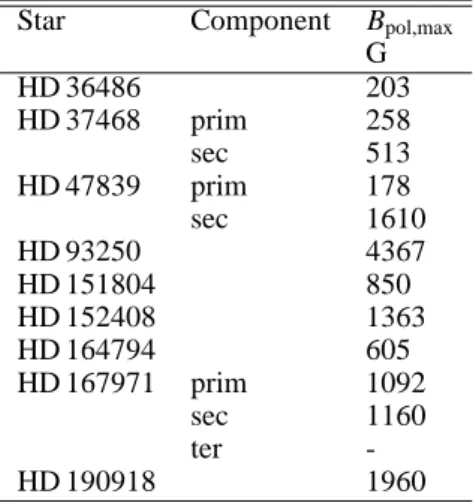
Table 4. Upper dipolar field strength limit in G, combining all available

data for each detected component of each star.

Star Component Bpol,max

G HD 36486 203 HD 37468 prim 258 sec 513 HD 47839 prim 178 sec 1610 HD 93250 4367 HD 151804 850 HD 152408 1363 HD 164794 605 HD 167971 prim 1092 sec 1160 ter -HD 190918 1960

the local thermal energy density (ζB) of 5 × 10−5, or between 30

and 5200 G if that ratio is assumed to be 0.5. In their work, the magnetic field strength scales with ζ_B1/2and Vrot.

The assumptions on the field configuration and slow rotation used by Parkin et al. (2014) are probably generally not adapted to PACWB. In particular, if the field is strong, the impact of the magnetic field on the wind, e.g. magnetic wind confine-ment, should be taken into account (ud-Doula & Owocki 2002; ud-Doula et al. 2008), and massive stars are often rapid rota-tors (e.g. Grunhut et al. 2013). Nevertheless, their work provides an idea of the typical field strengths that one might expect in PACWB.

Our analysis of archival spectropolarimetric data shows no magnetic detection in any of the 9 PACWB for which data are available. However, the precision reached by these archival ob-servations is between 7 and 211 G for the measured longitudinal field. These values are typical of the precision reached for the measurements of fields in massive stars by the MiMeS collab-oration (Grunhut et al., in prep.). Assuming an oblique dipole field, as observed in the vast majority of single massive stars, this leads to an upper limit of the undetected magnetic field at 3σ and a 90% probability of detection between 178 and 4367 G at the stellar pole, depending on the star.

While for some stars these archival observations are not really constraining (e.g. HD 93250), for several cases we can clearly exclude fields above 1000 G and thus large ζB values

are certainly not common in PACWB. The results obtained for HD 36486, HD 37468 and HD 47839 show that even dipolar fields above a few hundreds G, i.e. more moderate ζB, do not

seem common in PACWB, while this corresponds to the typi-cal field strength observed in magnetic massive stars (Petit et al. 2013). While the proportion of magnetic stars among OB stars (∼7%) could fit with the proportion of PACWB among massive binary stars, our results clearly show that PACWB are not par-ticularly magnetic compared to other massive stars. Therefore, no link could be established between the presence of a magnetic field typical of a magnetic massive star and the presence of syn-chrotron emission.

These archival data can however not exclude fields of a few tens of G or lower. Such field values would point towards low ζB

values and would be sufficient to produce synchrotron emission. However, studies of magnetism in OB stars show that magnetic fields detected in these stars are always relatively strong (with Bl

> 100 G). Weak magnetic fields are generally not found in

mas-sive stars, even when low detection thresholds are used. This is known as the magnetic dichotomy in massive stars (Aurière et al. 2007; Lignières et al. 2014).

However, ultra weak magnetic fields have recently been detected in some A stars (Lignières et al. 2009; Petit et al. 2011; Blazère et al. 2014). These fields could possibly also exist in higher mass stars, although attempts to detect them in B stars have been unsuccessful so far (Neiner et al. 2014; Wade et al. 2014a). Magnetic field amplification could exist in PACWB (Lucek & Bell 2000; Bell & Lucek 2001; Falceta-Gonçalves & Abraham 2012) and ultra weak stellar sur-face magnetic field could then be sufficient to produce syn-chrotron emission.

As a consequence, while this work represents the first ever effort to detect magnetic field signatures in PACWB, provide quantitative estimates of its possible value and constraints for models, and clearly excludes the presence of magnetic fields typical of massive stars as the origin of synchrotron emission in PACWB, more precise spectropolarimetric measurements of magnetic fields in PACWB are necessary before one can ex-clude the presence of very weak magnetic fields at the surface of PACWB stars. We plan to acquire such precise observations for very bright PACWB in the near future.

Nevertheless, even if ultra weak magnetic fields were present at the surface of PACWB and magnetic field amplification was at work, the question remains: if PACWB are not different, as far as their magnetic field is concerned, from typical massive stars, why are they particle accelerators? A possible scenario would be the production of a magnetic field at the location of the wind shock itself.

Acknowledgements. This research has made use of the SIMBAD database

op-erated at CDS, Strasbourg (France), and of NASA’s Astrophysics Data System (ADS). We thank the referee, M. Leutenegger, for his constructive feedback.

References

Aurière, M., Wade, G. A., Silvester, J., et al. 2007, A&A, 475, 1053 Bell, A. R. & Lucek, S. G. 2001, MNRAS, 321, 433

Blazère, A., Petit, P., Lignières, F., et al. 2014, ArXiv e-prints 1410.1412 Cazorla, C., Nazé, Y., & Rauw, G. 2014, A&A, 561, A92

De Becker, M., Pittard, J. M., Williams, P., & WR140 Consortium. 2011, Bul-letin de la Societe Royale des Sciences de Liege, 80, 653

De Becker, M. & Raucq, F. 2013, A&A, 558, A28

de la Chevrotière, A., St-Louis, N., Moffat, A. F. J., & MiMeS Collaboration. 2014, ApJ, 781, 73

Donati, J.-F., Semel, M., Carter, B. D., Rees, D. E., & Collier Cameron, A. 1997, MNRAS, 291, 658

Dougherty, S. M., Pittard, J. M., Kasian, L., et al. 2003, A&A, 409, 217 Dzib, S. A., Rodríguez, L. F., Loinard, L., et al. 2013, ApJ, 763, 139 Falceta-Gonçalves, D. & Abraham, Z. 2012, MNRAS, 423, 1562 Farnier, C., Walter, R., & Leyder, J.-C. 2011, A&A, 526, A57

Gray, D. F. 2005, The Observation and Analysis of Stellar Photospheres (Cam-bridge University Press)

Grunhut, J. H., Wade, G. A., Leutenegger, M., et al. 2013, MNRAS, 428, 1686 Harvin, J. A., Gies, D. R., Bagnuolo, Jr., W. G., Penny, L. R., & Thaller, M. L.

2002, ApJ, 565, 1216

Helstrom, C. W. 1995, Elements of Signal Detection and Estimation (Prentice Hall)

Jardine, M., Allen, H. R., & Pollock, A. M. T. 1996, A&A, 314, 594

Kay, S. M. 1998, Fundamentals of Statistical Signal Processing, Volume 2: De-tection Theory (Prentice Hall)

Kupka, F., Piskunov, N., Ryabchikova, T. A., Stempels, H. C., & Weiss, W. W. 1999, A&AS, 138, 119

Levy, B. C. 2008, Principles of Signal Detection and Parameter Estimation (Springer)

Lignières, F., Petit, P., Aurière, M., Wade, G. A., & Böhm, T. 2014, in IAU Symposium, Vol. 302, IAU Symposium, 338

Lignières, F., Petit, P., Böhm, T., & Aurière, M. 2009, A&A, 500, L41 Lucek, S. G. & Bell, A. R. 2000, MNRAS, 314, 65

Markwardt, C. B. 2009, in Astronomical Society of the Pacific Conference Se-ries, Vol. 411, Astronomical Data Analysis Software and Systems XVIII, ed. D. A. Bohlender, D. Durand, & P. Dowler, 251

Mason, B. D., Gies, D. R., Hartkopf, W. I., et al. 1998, AJ, 115, 821

Moré, J. 1978, in Lecture Notes in Mathematics, Vol. 630, Numerical Analysis, ed. G. Watson (Springer Berlin Heidelberg), 105

Nazé, Y., Bagnulo, S., Petit, V., et al. 2012, MNRAS, 423, 3413

Neiner, C., Monin, D., Leroy, B., Mathis, S., & Bohlender, D. 2014, A&A, 562, A59

Parkin, E. R., Pittard, J. M., Nazé, Y., & Blomme, R. 2014, ArXiv e-prints 1406.5692

Petit, P., Lignières, F., Aurière, M., et al. 2011, A&A, 532, L13 Petit, V., Owocki, S. P., Wade, G. A., et al. 2013, MNRAS, 429, 398

Piskunov, N. E., Kupka, F., Ryabchikova, T. A., Weiss, W. W., & Jeffery, C. S. 1995, A&AS, 112, 525

Pittard, J. M., Dougherty, S. M., Coker, R. F., O’Connor, E., & Bolingbroke, N. J. 2006, A&A, 446, 1001

Rauw, G., Sana, H., Spano, M., et al. 2012, A&A, 542, A95 Rees, D. E. & Semel, M. D. 1979, A&A, 74, 1

Sana, H., de Mink, S. E., de Koter, A., et al. 2012, Science, 337, 444 Sana, H., Le Bouquin, J.-B., De Becker, M., et al. 2011, ApJ, 740, L43 Sana, H., Le Bouquin, J.-B., Lacour, S., et al. 2014, ArXiv e-prints 1409.6304 Simón-Díaz, S. & Herrero, A. 2014, A&A, 562, A135

ud-Doula, A. & Owocki, S. P. 2002, ApJ, 576, 413

ud-Doula, A., Owocki, S. P., & Townsend, R. H. D. 2008, MNRAS, 385, 97 Wade, G. A., Donati, J.-F., Landstreet, J. D., & Shorlin, S. L. S. 2000, MNRAS,

313, 851

Wade, G. A., Folsom, C. P., Petit, P., et al. 2014a, MNRAS, 444, 1993 Wade, G. A., Grunhut, J., Alecian, E., et al. 2014b, in IAU Symposium, Vol. 302,