HAL Id: hal-01548193
https://hal.archives-ouvertes.fr/hal-01548193
Submitted on 27 Jun 2017
HAL is a multi-disciplinary open access archive for the deposit and dissemination of sci-entific research documents, whether they are pub-lished or not. The documents may come from teaching and research institutions in France or abroad, or from public or private research centers.
L’archive ouverte pluridisciplinaire HAL, est destinée au dépôt et à la diffusion de documents scientifiques de niveau recherche, publiés ou non, émanant des établissements d’enseignement et de recherche français ou étrangers, des laboratoires publics ou privés.
National borders matter...where one draws the lines too
Vincent Vicard, Emmanuelle Lavallée
To cite this version:
Vincent Vicard, Emmanuelle Lavallée. National borders matter...where one draws the lines too. Cana-dian Journal of Economics, 2013, 46 (1), pp.135-153. �10.1111/caje.12008�. �hal-01548193�
DOCUMENT
DE TRAVAIL
N° 272
DIRECTION GÉNÉRALE DES ÉTUDES ET DES RELATIONS INTERNATIONALES
NATIONAL BORDERS MATTER...WHERE ONE
DRAWS THE LINES TOO
Emmanuelle Lavallée and Vincent Vicard
DIRECTION GÉNÉRALE DES ÉTUDES ET DES RELATIONS INTERNATIONALES
NATIONAL BORDERS MATTER...WHERE ONE
DRAWS THE LINES TOO
Emmanuelle Lavallée and Vincent Vicard
January 2010
Les Documents de travail reflètent les idées personnelles de leurs auteurs et n'expriment pas nécessairement la position de la Banque de France. Ce document est disponible sur le site internet de la
Banque de France « www.banque-france.fr ».
Working Papers reflect the opinions of the authors and do not necessarily express the views of the Banque
National borders matter...where one draws the lines too
∗ Emmanuelle Lavall´ee† Vincent Vicard‡January 2010
∗We would like to thank Adeline Bachellerie, Pierre-Philippe Combes, Lionel Fontagn´e, Luke Haywood,
Philippe Martin, Thierry Mayer and seminar participant in University Paris I and Banque de France for their helpful suggestions.
†University Paris-Dauphine, LEDa and DIAL (Developpement, Institution et Analyse de long terme).
E-mail: [email protected]
Abstract
The fact that crossing a political border dramatically reduces trade flows has been widely documented in the literature. The increasing number of borders has surprisingly attracted much less attention. The number of independent countries has indeed risen from 72 in 1948 to 192 today. This paper estimates the effect of political disintegration since World War II on the measured growth in world trade. We first show that trade statistics should be considered carefully when assessing globalization over time, since the definition of trade partners varies over time. We document a sizeable resulting accounting artefact, which accounts for 17% of the growth in world trade since 1948. Second, we estimate that political disintegration alone since World War II has raised measured international trade flows by 9% but decreased actual trade flows (including inter-regional trade) by 4%.
JEL classification: F1, N70.
Keywords: Trade, Borders, Political disintegration, Trade statistics.
R´esum´e
De nombreux articles r´ecents montrent que le passage d’une fronti`ere politique r´eduit fortement les ´echanges. L’augmentation du nombre de fronti`eres et ses cons´equences pour le commerce international n’ont pas fait l’objet de la mˆeme d’attention dans la litt´erature. Le nombre d’´Etats souverains a pourtant augment´e de 72 en 1948 `a 192 aujourd’hui. Cet article estime l’effet de la d´esint´egration politique sur la mesure de la croissance du commerce mondial depuis la seconde guerre mondiale. Notre analyse souligne d’abord que les statistiques commerciales doivent ˆetre trait´ees avec prudence lorsque l’on mesure l’´evolution du degr´e de mondialisation, car la d´efinition des parte-naires commerciaux varie dans le temps. Il en r´esulte un biais statistique important, qui explique 17% de la croissance du commerce international depuis 1948. Nous mon-trons ensuite que l’augmentation du nombre d’´Etats souverains seule a entrain´e une augmentation du commerce international mesur´e de 9%, mais a en r´ealit´e diminu´e les ´echanges (incluant le commerce interr´egional) de 4%.
Code JEL: F1, N70.
Mots cl´es: Commerce international, Fronti`eres, D´esint´egration politique, Statistiques com-merciales.
I
Introduction
International trade has grown almost twice as fast as world income since World War II, leading to an increase in the trade to GDP ratio from 24% in 1960 to 48% in 2003. The causes of economic globalization remain surprisingly disputed (Krugman,1995). The usual suspects put forward in the literature are decreasing transport costs and the removal of tariffs and non-tariff barriers to trade. Hummels(2007) nevertheless finds little systematic evidence documenting the decline in transport costs. He shows that, whereas air shipping experienced a sharp cost reduction between 1955 and 2004, ocean shipping, which accounts for 99% of world trade by weight, did not register such a decline.1
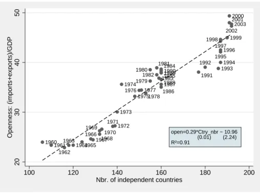
These explanations relate to the dissolution of national borders, either because of technological progress in transport and communication or of the worldwide implementation of free trade policies. A third explanation relates to the drawing of political borders. As stated byKrugman(1995, p.340), “if international trade only includes shipments that cross the borders, it is clear that the volume of trade depends quite a lot on where one draws the line”. In this respect, an outstanding feature of the past five decades is the increasing number of sovereign nations. The number of countries has indeed increased from 72 in 1948 to 192 today, thanks in particular to the decolonization process and the break-up of the Soviet Union. Figure 1 clearly suggests that the number of independent countries and global trade openness measured by export plus imports over GDP are correlated.2
The aim of this paper is to investigate how and to what extent political disintegration has affected the volume and geography of world trade since World War II.
The break-up of nations affects international trade through three channels. On the one hand, former intra-national trade flows become international trade flows. Since these shipments existed before independence, recording them as international flows creates an accounting artefact in the measurement of international trade over time. Moreover, pairs of countries ever in a colonial relationship or former members of the same country share linkages and economic, cultural and institutional characteristics that make them trade more than average pairs of countries (Rose,2000;de Sousa and Lamotte,2007;Head et al.,
2007). On the other hand, the creation of political borders change relative trade costs. It creates impediments to trade - tariffs as well as non-tariffs barriers to international flows such as independent currencies or different standards and competition policies (Anderson and van Wincoop, 2004) - that dramatically reduce international trade in comparison to
1Hummels et al.(2001) nevertheless show than small decreases in trade costs can lead to large increases
in the volume of trade by fostering vertical specialization.
2Alesina et al.(2000) argue that trade liberalization leads to political disintegration because being able
to trade easily with the rest of the world decreases the advantage of having a large domestic market. They link political disintegration to the level of world trade freeness, while our paper links political disintegration to the observed volume of international trade for a given level of world trade freeness.
Figure 1: Number of independent countries in the world and global trade openness 1960 1961 1962 1963 19641965 1966 19671968 1969 1970 1971 1972 1973 1974 1975 1976 1977 1978 1979 1980 1981 1982 1983 1984 1985 1986 1987 1988 1989 1990 1991 1992 1993 1994 1995 1996 1997 1998 1999 2000 2001 2002 2003 open=0.29*Ctry_nbr − 10.96 (0.01) (2.24) R²=0.91 20 30 40 50 Openness: (imports+exports)/GDP 100 120 140 160 180 200 Nbr. of independent countries
Source: World Bank and the Correlates of War project
intra-national trade (McCallum,1995; Anderson and van Wincoop, 2003). Finally, since bilateral trade flows depend on relative trade costs (Anderson and van Wincoop, 2003), creating border barriers with some partners should increase trade with other partners. For instance, the Czech Republic would be expected to trade less with Slovakia after the break-up of Czechoslovakia, but more with any third country.
The contribution of this paper is threefold. We first provide an assessment of the growth in international trade since World War II due to the variation over time in the sample of countries recorded in the international statistics. We show that this accounting artefact is sizeable and accounts for one sixth in the growth of measured international trade since World War II. Part of the accounting artefact comes from the fact that the trade flows of some former colonies were not recorded at all in international statistics (neither independently nor as part of their colonizer’s trade) up to their independence. Second, we investigate the impact of the creation of new political borders alone on the volume and geography of world trade since World War II. Based on a theoretically motivated gravity model of trade, we estimate world trade flows in 2005 and in a counterfactual world in 2005 with 1945 borders. We show that newly independent states trade less with former members of the same country (or their former colonizer) but trade more with the rest of the world. Overall, our empirical results suggest that political disintegration has increased measured international trade flows by 9% but decreased actual (including inter-regional)
trade flows by 4%. Third, we show that the distribution of GDP abroad affects a country’s trade to GDP ratio; a country’s trade openness increases when GDP abroad is distributed among a larger number of trade partners.
Several papers investigate the causes of the growth in world trade as a share of GDP.
Estevadeordal et al.(2003) study the causes of the rise and fall of the trade to output ratio during the 1870-1939 period. They show that the driving forces of trade globalization were a fall in transport costs and the rise of the gold standard. Rose (1991) and Baier and Bergstrand(2001) focus on the second wave of globalization after World War II. They both work on a sample of OECD countries. Baier and Bergstrand (2001) show that two thirds of the growth in trade between the late 1960s and the late 1980s can be explained by income growth, 25% by a reduction in tariffs and 8% by a decline in transport costs.3
All these papers investigate the determinants of international trade growth on a subset of countries, i.e. they investigate the intensive margin of the growth in international trade. They cannot address the effect of the change in underlying features of the data such as the distribution of GDP among an increasing number of potential trading partners, i.e. the extensive margin of the growth in international trade. Yet world trade has increased by a factor of 30 between 1948 and 2007, while over the same period trade between OECD countries4has increased by a factor of only 20. At the same time, the international trading
system has expanded from 72 × 71/2 = 2556 potential bilateral trade relationships in 1948 to 192 × 191/2 = 18336 today. Assessing the contribution of this extensive margin to the growth in international trade requires a structural estimation of a theoretically motivated gravity model.
The paper proceeds as follows. The next section provides evidence and estimates of the accounting artefact related to variations over time in countries reported in interna-tional trade statistics. The third section presents a theoretically based gravity framework allowing the estimation of the impact of border changes on the geography and volume of world trade flows. Section 4 reports the estimation results.
II
An assessment of the accounting artefact
The assessment of globalization through measured world trade depends crucially on the number of trade partners considered:
MW = X i∈N X j∈N,j6=i Mij (1)
3Jacks et al.(2009) confirm the prevalence of decreasing trade costs during the first wave of globalization
and of income growth during the second.
where MW denotes world imports and Mij imports of i from j. Aggregate international trade depends on the set of declaring exporters and importers N . In this section, we estimate how variations over time in the sample of trade partners affect measured trade growth since World War II.
We use the declared imports in the Direction of Trade Statistics (DOTS) database of the International Monetary Fund, which provides data on bilateral merchandise trade over the period 1948-2007. The DOTS database is the main source of international trade data available over a long time span.
1 Independent states and trade partners in the DOTS
The DOTS database reports trade flows between “entities” that are not necessarily in-dependent countries as defined by international law and practice. As put forward by
Russett et al. (1968) and Small and Singer (1982, p38-46), in order to be registered as a state member of the international system, “the entity must be a member of the United Nations or League of Nations, or have population greater than 500,000 and receive diplo-matic missions from two major powers”.5 Trade partners in the DOTS database include
some territorial entities that are not independent states, and some independent states are not considered as trade partners.
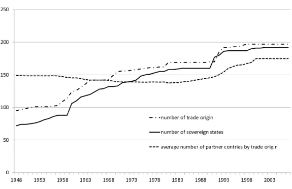
Figure2illustrates the discrepancy between the number of independent states and the number of trade partners in the DOTS. For instance, in 2000, 191 states were recognized as sovereign nations, while 195 trade origins (i.e. entities reporting imports) were recorded in the DOTS. This discrepancy is due to the fact that some independent countries (Taiwan, Monaco, Andorra, Liechtenstein, Botswana, Lesotho, Namibia and Swaziland6) were not
taken into account whereas some territorial entities, that were not sovereign states, were.7 In addition, Figure 2 underlines that the DOTS matrix is not squared, since the number of declared trade partners varies by trade origin and increases over time.
From 1948 to 2007, 120 countries became independent but only 102 new trade origins were created (Figure 2). Three quarters of these new trade origins reflect the creation of a new sovereign state, through the decolonization process (53%) and the break-up of nations (21%). The remaining 26% are related to the recognition of existing countries in 1948, such as Mongolia or Afghanistan, and territories that are still not sovereign, like the overseas territories of France, United Kingdom or the Kingdom of the Netherlands.8 The
5”State System Membership List Codebook”, Version 2004.1 http://www.correlatesofwar.org/ 6The DOTS does not consider Botswana, Lesotho, Namibia and Swaziland as trade origins but rather the South African Common Customs Area (SACCA) excluding South Africa.
7Aruba, Bermuda, Hong Kong, Macao, Faeroe Islands, the Falkland Islands, French Polynesia, Green-land, the Netherlands Antilles, New Caledonia and St Pierre et Miquelon.
Figure 2: Sovereign states, trade origins and trade partners
size of the DOTS matrix has accordingly been multiplied by more than two.
The size of the DOTS matrix therefore depends to a large extent on changes in political borders over time. New independent countries, however, did not necessarily enter the DOTS in the years following their independence. Some colonies were already taken into account in the DOTS in 1948 (see Table 1). Subsequently, in half of the cases, a new independent country was recorded as a trade origin before its independence.
Table 1: Entities reporting to the DOTS in 1948 although they were not independent
Algeria 1962 (FR) Kenya 1963 (UK) Sierra Leone 1961 (UK) Angola 1975 (PR) Laos 1949 (FR) Sudan 1956 (UK, Egypt) Cambodia 1953 (FR) Madagascar 1960 (FR) Suriname 1975 (Nth)
Cameroon 1960 (FR-UN) Malaysia 1957 (UK) Trinidad & Tobago 1962 (UK) Congo, D. R. 1960 (Bel) Malta 1964 (UK) Tunisia 1956 (FR)
Cyprus 1960 (UK) Mauritius 1968 (UK) Uganda 1962 (UK) Ghana 1957 (UK) Morocco 1956 (FR) Vietnam 1953 (FR) Guyana 1966 (UK) Mozambique 1975 (PR) Zambia 1964 (UK) Jamaica 1962 (UK) Nigeria 1960 (UK) Zimbabwe 1980 (UK) Notes: Colonizer in parenthesis. Date of independence are taken from Correlates of War Project. 2005. “State System Membership List, v2004.1”
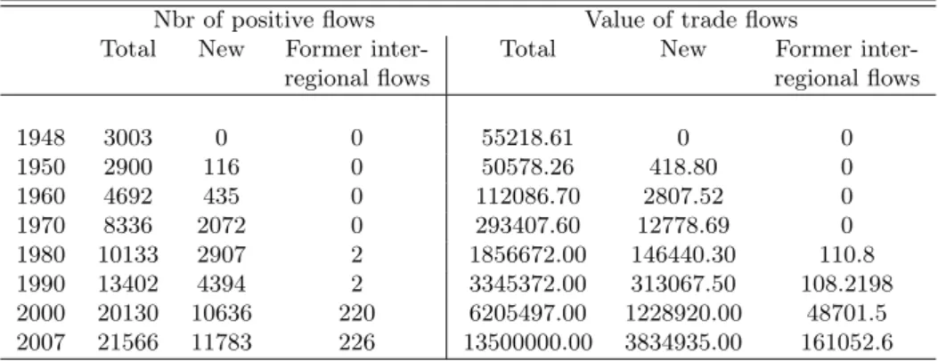
Since 1948, the number of effective (positive) bilateral trade flows has been continuously growing and has increased more than six-fold over the period. New trade flows (i.e. involving a new trade origin and/or partner) represent an increasing share of bilateral
five French overseas departments (Guadeloupe, Guyana, Martinique, Reunion and French Guiana) were considered as distinct trade origins even if they were (and still are) part of France. On the contrary, Belgium and Luxembourg were recorded as a single trade partner from 1948 to 1996.
trade flows, from 4% in 1950 to 55% in 2007 (see Figure3 and Table 2).9 In comparison,
the share of trade flows between countries that used to belong to the same statistical entity made up 1% of world trade transactions in 2007 (see table2). The value of trade flows involving new entities has also increased dramatically, to stand at 28% in the 2007.
Table 2: Number and value of world trade flows by decade
Nbr of positive flows Value of trade flows
Total New Former inter- Total New Former
inter-regional flows regional flows
1948 3003 0 0 55218.61 0 0 1950 2900 116 0 50578.26 418.80 0 1960 4692 435 0 112086.70 2807.52 0 1970 8336 2072 0 293407.60 12778.69 0 1980 10133 2907 2 1856672.00 146440.30 110.8 1990 13402 4394 2 3345372.00 313067.50 108.2198 2000 20130 10636 220 6205497.00 1228920.00 48701.5 2007 21566 11783 226 13500000.00 3834935.00 161052.6 Notes: Authors’ calculations on the basis of DOTS.
Figure 3: Number of trade flows from 1948 to 2007
9Felbermayr and Kohler(2006) show that the share of positive trade flows in the total number of flows
has remained fairly constant over time and distinguish the contribution of new flows between existing trade origin in 1948 and flows involving a new trade origin.
2 Estimating the accounting artefact
Whatever its cause, the creation of a new trade origin or trade partner in the DOTS automatically increases the world trade matrix and thus international trade. Two cases should nevertheless be distinguished regarding the statistical artefact which is generated on the measurement of international trade.
In the general case of a country break-up, former inter-regional trade flows become international flows because former regions of the same country become sovereign nations.10 For instance, the break-up of Czechoslovakia in 1993 resulted in the creation of two new countries: the Czech Republic and Slovakia. Czechoslovakian trade, however, included the trade of all its regions with the rest of the world. In this case, we thus define trade flows between the Czech Republic and Slovakia (i.e. USD 4882 millions in 1993) as a statistical artefact since they existed before independence but were not recorded in the DOTS.
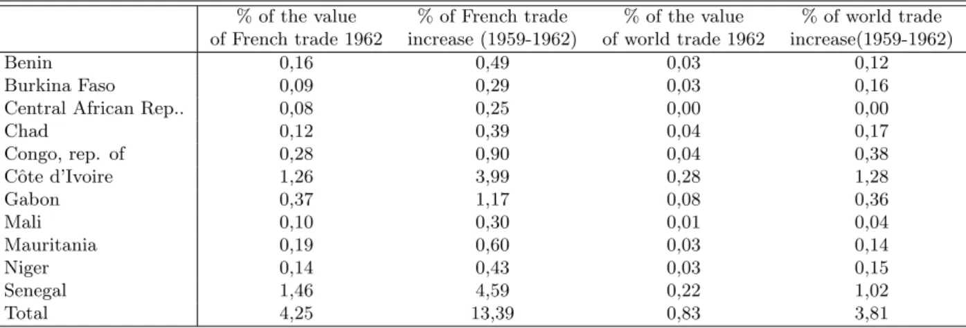
A country’s independence may nevertheless have more severe consequences on the measurement of international trade. The trade of some independent states, territories or colonies was simply not recorded at all in international trade statistics before their independence or their creation as a trade origin. In this case, all trade flows of these countries contribute to the accounting artefact since they existed but were not recorded in 1948 and appeared in international statistics between 1948 and 2007. To illustrate the relevance of this second source of accounting artefact, let’s consider the case of the former French West and Equatorial African colonies, whose trade flows were simply not included in the DOTS database even as part of the French imports or exports.11 Table3shows that
in 1962 these countries represented 4.25% of French foreign trade and that, from 1959 to 1962, their independence and creation as a trade origin accounted for 13.4% of the increase in French trade. In addition, although they represented less than one percent of world trade in 1962, their creation accounted for almost 4% of the increase in the value of world trade flows between 1959 and 1962.
The accounting artefact is sizeable also at the world level. In order to assess the bias introduced in world trade statistics by the creation of new trade origins and trade partners, we compute the share of the growth in world trade due to flows that were not recorded as international trade flows in 1948. More precisely, we subtract from the total value of imports recorded in the DOTS since 1948 the total value of trade between country pairs
10As mentioned previously trade origins in the DOTS are not necessarily independent states, and their definition has changed over time. Such changes are not neutral in term of measured international trade. For instance, from 1948 to 1996 Belgium and Luxembourg were considered as a single trade partner. In 1997, these two countries were for the first time considered as distinct trade partners, and their bilateral trade recorded in the DOTS.
11The French Customs and Excise Department (1959) defines the French statistical territory as conti-nental France (including the free zones of pays de Gex and Haute-Savoie), Corsica, Monaco and Sarre.
Table 3: Impact on French and world trade of the independence of French Western and Equatorial Africa (1959-1962)
% of the value % of French trade % of the value % of world trade of French trade 1962 increase (1959-1962) of world trade 1962 increase(1959-1962)
Benin 0,16 0,49 0,03 0,12
Burkina Faso 0,09 0,29 0,03 0,16
Central African Rep.. 0,08 0,25 0,00 0,00
Chad 0,12 0,39 0,04 0,17 Congo, rep. of 0,28 0,90 0,04 0,38 Cˆote d’Ivoire 1,26 3,99 0,28 1,28 Gabon 0,37 1,17 0,08 0,36 Mali 0,10 0,30 0,01 0,04 Mauritania 0,19 0,60 0,03 0,14 Niger 0,14 0,43 0,03 0,15 Senegal 1,46 4,59 0,22 1,02 Total 4,25 13,39 0,83 3,81
Notes: Authors’ calculations on the basis of DOTS.
that were not recorded in the DOTS trade matrix in 1948. Our definition includes country pairs that used to belong to the same country (e.g. Czech Republic and Slovakia) and country pairs that were not recorded in 1948 either because the importer was not recorded as a trade origin in the DOTS in 1948 (e.g. Afghanistan, Mali) or because the exporter was not declared as a trade partner by a particular trade origin. Note that our definition of the accounting artefact is restrictive since we consider as existing all country pairs recorded in the DOTS in 1948, including those for which a zero or missing value is reported in 1948 (79% of observations).12 Accordingly, our quantification of the accounting artefact
excludes the ‘real’ extensive margin, i.e. zero trade flows between existing country pairs in 1948 that subsequently turned positive.
Results in Table4confirm that the accounting artefact is sizeable: it accounts for more than one sixth of the growth in world trade since World War II. The accounting artefact was particularly significant in the 1950s and 1960s due to the decolonization process and in the 1990s due to the break-up of the Soviet Union.13 Overall, 17% of world trade growth
since 1948 is related to the inclusion of new trade origins in the DOTS database.
This section shows that variations over time in the number and definition of trade origins and partners in international trade statistics inflate the measured growth in inter-national trade. As underlined above, the creation of a new trade origin does not necessarily reflect the recognition of a new sovereign state. Moreover, changing political borders may
12Gleditch(2002) argues that many zeros in the DOTS are problematic and should be treated as missing
observations.
13Note that the German reunification has had no effect on the accounting artefact since trade flows between the Federal Republic of Germany and the German Democratic Republic was null before reunifi-cation.
Table 4: Assessing the accounting artefact
Value of trade flows Artificial trade creation (millions of constant USD) (share of total trade growth)
total artefact cumulative by decade
1948 229123 0 1959 334141 8334 7.9 7.9 1960 378671 9459 1969 690125 30266 6.6 3.2 1970 756205 32844 1979 2095359 162439 8.7 0.9 1980 2253243 174605 1989 2381311 235550 10.9 2.0 1990 2559581 236689 1999 3308888 335612 10.9 9.5 2000 3603657 395374 2007 6510982 1083380 17.2 0.3
Notes: Authors’ calculations on the basis of DOTS. The last column reports the statistical artefact related to new trade origins/partners created during the decade only.
affect trade with third countries. Fully quantifying the contribution of changing political borders on the growth in world trade therefore requires to go beyond simple descriptive statistics and to structurally estimate a trade model. In the next section, we investigate the impact of changing political borders on the volume and geography of world trade based on a micro-founded gravity model of trade `a laAnderson and van Wincoop (2003).
III
The gravity model and borders
The gravity model of trade is based on two building blocks (Anderson and van Wincoop,
2003). Consider first N countries/regions each specialized in the production of one good differentiated by place of origin. We assume the supply of each good to be fixed. Let then add identical, homothetic preferences represented by the following CES utility function:
Uj =
X
i∈N
c(σ−1)/σij (2)
where cij is consumption of goods produced in country i by consumer of country j and
σ is the elasticity of substitution between all goods. Country j’s consumers maximise (2) subject to the budget constraint:
X
i∈N
pijcij = yj (3)
where pij is the price of goods produced in country i for country j’s consumers and yj is
Let tij be the variable trade costs on exports from i to j. Then pij = pitij where pi is country i’s supply price. The value of exports from country i to country j is xij = pijcij
and total income of country i is yi =
P
j∈Nxij.
Maximization of (2) subject to (3) yields:
xij = µ pitij Pj ¶1−σ yj (4)
where Pj is given by:
Pj = Ã X i∈N (pitij)1−σ !1/(1−σ) . (5)
Market clearance implies:
yi= X j∈N xij = p1−σi X j∈N µ tij Pj ¶1−σ yj. (6)
FollowingAnderson and van Wincoop(2003), using (6) to solve for the unknown prices pi together with (4) and (5), we obtain:
xij = yiyj yw µ tij ΠiPj ¶1−σ (7) where Π1−σi = X j yj yw tij Pj 1−σ (8) Pj1−σ = Ã X i yi yw tij Πi !1−σ . (9)
1 World openness under free trade
Under free trade, i.e. without transport costs or tariffs so that prices are identical for all countries, bilateral trade is determined by the product of the two countries’ GDPs. The analysis of world trade is then straightforward: global trade openness depends only on the size distribution of countries. Since prices are identical for all countries, we normalize them to unity: pij = 1∀i, j. We thus have:
xij =
yiyj
yw = xji. (10)
of GDP traded inside the region is defined by: TA YA = sA Ã 1 −X i∈A (siA)2 ! (11)
where TA is the volume of intra-regional trade, YA is the regional GDP, sA is the share
of region A in world GDP and siA are the share of region A’s GDP of each country i in region A. At the world level,Helpman (1987)’s equation yields:
TW YW = Ã 1 −X i∈N (si)2 ! (12)
where TW is the volume of world trade, N is the total number of countries in the world
and si is i’s share of world GDP. The last term on the right hand side of (12) is a “size
dispersion index”. The latter is minimized for N identical countries whose share of world GDP is N1. Hence, under free trade, the relationship between global trade openness and the number of independent countries is straightforward: an increase in the number of countries increases the share of world production traded internationally by decreasing the “size dispersion index”.
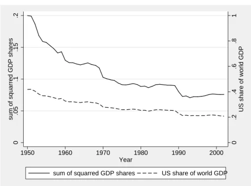
Figure4plots the evolution between 1950 and 2002 of the sum of the squared share of world GDP of independent countries and the US share of world GDP. It confirms that the size dispersion index has been declining since World War II, thanks in particular to the sharp decline of the US share of global GDP. The world with which the US were trading in 1950 was with an outside world slightly larger than itself but is now five times larger.
2 Gravity with trade barriers
With transport costs, the analysis is less straightforward since bilateral trade depends on relative trade costs (Anderson and van Wincoop, 2003). Any change in bilateral trade costs between two countries therefore affects the trade flows of each country with its other partners. A country break-up creates border barriers between former regions of the same country. This has two effects on international trade. First, it reduces actual trade flows between the two new independent countries but increases recorded international trade flows since trade between regions is not recorded as international trade before independence. Second, it increases the average trade barriers that new countries face with all their trading partners. A new independent country should thus trade less with the former regions of the same country but trade more with other partners.
Figure 4: Size distribution of countries 0 .2 .4 .6 .8 1 US share of world GDP 0 .05 .1 .15 .2
sum of squarred GDP shares
1950 1960 1970 1980 1990 2000
Year
sum of squarred GDP shares US share of world GDP
Source: Penn World Table 6.2
can be properly estimated using country fixed effects that account for inward and outward multilateral resistance terms Πi and Pj. We can therefore consistently estimate the effect of national independence on trade between two former members of the same country from (7). However, to assess the effect of country break-ups on trade with other partners, we need to compute the multilateral resistance terms from (8) and (9).
Assuming symmetric trade barriers, tij = tji, we have Πi = Pi, and:
Pj1−σ =X
i
Piσ−1 yi
ywt1−σij ∀j. (13)
We assume the following trade cost function:
ln tij = ln distij+
X
h
αhzh. (14)
The vector of observable bilateral linkages affecting trade costs includes variables measur-ing geographical, cultural and historical proximity as well as trade policy variables:
Zij = [Contigij, Langij, Smctryij, Colonyij, ComColij, Comcurij, RT AijW T Oij] (15)
where Contigij, Langij and Comcurij are dummies for countries sharing a common
measure common membership of a regional trade agreement and the World Trade Orga-nization, and Smctryij, Colonyij and ComColij are dummies equal to 1 for, respectively,
regions of the same country, countries ever in a colonial relationship and sharing a common colonizer since World War II.
So we have: Pj1−σ =X i Piσ−1yi yw expβ1ln distij+ P hβhzh. (16)
The β’s coefficients in (16) may be consistently estimated from (7). We may then solve the vector of Pj1−σ using the system of N goods market equilibrium conditions (16), estimated coefficients from (5) and GDP shares. We are thus able to estimate the impact of the establishment of a political border on trade with former regions of the same country and with the rest of the world.
IV
Empirics
Our empirical strategy consists of three steps. First, we need to estimate the impact of the components of the trade cost vector using a gravity equation with country fixed effects. Second, we solve the vector of Pj1−σ using the system of N goods market equilibrium conditions (16). Then we estimate bilateral trade flows in 2005 and for a counterfactual world in 2005 with 1945 borders. To be clear about our approach, our aim is not to compare world trade flows in 2005 to those in 1945 but world trade flows in 2005 to those that would have prevailed, all other things being equal, in 2005 should the political borders have remained the same as in 1945.
1 Data
Trade flows are taken from the Direction of Trade Statistics (DOTS) database of the In-ternational Monetary Fund. GDP data are from the World Bank’s World Development Indicators (WDI). The data on regional trade agreements originates from Vicard (2009) and data on currency unions are an extended version ofGlick and Rose (2002) available athttp://jdesousa.univ.free.fr/data.htm. Data on geographical distances and com-mon official language come from the CEPII database14. The data on sovereign nations
and colonial relationships are taken from the Correlates of War project15 and completed by the CIA World Factbook. We consider countries that had a direct colonial link and
14http://www.cepii.fr/francgraph/bdd/distances.htm
15Correlates of War Project. 2005. “State System Membership List, v2004.1” and “Colonial/Dependency Contiguity Data, 1816-2002. Version 3.0.” http://www.correlatesofwar.org/.
countries that used to belong to the same country (Czech Republic and Slovakia) as a single category (Colonyij). We define a second category for countries sharing a common
colonizer (ComColij).16
2 Same country effect
In this section, we take advantage of the discrepancy between sovereign nations and entities in the DOTS to estimate the impact on bilateral trade of belonging to the same country. In 2005, the DOTS database reports trade flows for 20 entities that are not sovereign states.17
Substituting trade costs (14) into (7) and log-linearizing, we obtain the following econo-metric model:
ln xij = β1ln distij+ β2Contigij + β3Langij+ β4Smctryij + β5Colonyij + β6ComColij
+β7Comcurij + β8RT Aij + γ|1ln y{zi+ γ2P}i Ii
+ γ|3ln yj{z+ γ4P}j Ei
+εij (17)
where Ii and Ei are importer’s and exporter’s fixed effects and εij is the error term.
The estimation of (17) by OLS may indeed yield biased estimates: because of Jensen’s inequality (E(lnε) 6= lnE(ε)). Santos Silva and Tenreyro (2006) show that estimating gravity equations in the standard log-linear form yields biased parameter estimates. They suggest using a Poisson quasi maximum likelihood (PQML) estimator, which yields con-sistent estimates in the presence of heteroscedasticity. The PQML technique also enables us to avoid dropping zero trade values, which represent 31% of observations in our dataset. We thus estimate (17) in exponential form on a cross-section in 2005 using a PQML esti-mator.
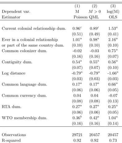
Results are presented in column (1) of Table 5. The coefficients on standard gravity variables are in line with the literature. The coefficient on the common colonizer dummy is however not significant. Since we work on a cross-section in 2005, colonial business linkages may have vanished since independence (Head et al., 2007). However, when we include a dummy for countries sharing a common colonizer and still in an ongoing colonial
16These definitions slightly differ from those adopted inRose(2000) orHead et al.(2007). For instance, Mali and Cˆote d’Ivoire were part of French West Africa before their independence. Each of them had a direct colonial link with France, but they were also part of the same territorial entity. Mali and Cˆote d’Ivoire are accordingly included in Colonyijinstead of ComColij.
17These entities are small and remote from the rest of the country they belong to. Our results should accordingly not be regarded as an estimation of the border effect put forward byMcCallum(1995) and
Anderson and van Wincoop(2003) using data on Canadian provinces and US States. They are however
much more representative of the “border effect” between colonies and colonizer, since most colonies were also small and remote from their colonizer.
relationship, its coefficient is also insignificant, confirming the insignificance of common colonial history for trade relationships after independence. The inclusion of country fixed effects controlling for legal origin may however partially explain this result. Finally, the insignificant coefficient on the common currency dummy may reflect the fact that we consider the euro together with other common currencies without a long panel dataset (Frankel,2008).
Table 5: Gravity results
(1) (2) (3)
Dependent var. M M > 0 log(M)
Estimator Poisson QML OLS
Current colonial relationship dum. 0.96c 0.89c 1.53a
(0.51) (0.49) (0.41) Ever in a colonial relationship 1.01a 0.98a 2.16a
or part of the same country dum. (0.10) (0.10) (0.10) Common colonizer dum. -0.02 -0.03 0.75a
(0.16) (0.16) (0.07) Contiguity dum. 0.54a 0.55a 0.56a
(0.07) (0.07) (0.10) Log distance -0.79a -0.79a -1.66a
(0.03) (0.03) (0.03) Common language dum. 0.17a 0.17a 0.66a
(0.06) (0.06) (0.05) Common currency dum. 0.04 0.04 -0.07
(0.08) (0.08) (0.13)
RTA dum. 0.27a 0.27a 0.25a
(0.06) (0.06) (0.05) WTO membership dum. 0.36b 0.42a 1.04a
(0.16) (0.16) (0.14)
Observations 29721 20457 20457
R-squared 0.92 0.92 0.73
Notes: a, b, c denotes significance at the 1, 5 and 10% level. Heteroscedasticity-robust standard errors are in parenthesis.
Countries that have ever been in a colonial relationship or part of the same country since 1945 trade 175% more than other country pairs, while regions currently in a colonial relationship trade on average e1.01+0.96− 1 = 616% more.18 Our estimates are
conserva-tive with respect to the literature exploring the impact of colonial history and country break-up on trade. Rose(2000) shows in his benchmark results for 1990 that the colonial relationship raises bilateral trade by a factor of 5.75, all other things being equal, while having had a common colonizer makes countries bilateral trade 80% larger. Papers dealing directly with the break-up of nations or colonial empires show that country break-up
matically decreases bilateral trade. For instance, Fidrmuc and Fidrmuc (2003) find that, at the time of their independence, the Czech Republic and Slovakia were trading 43 times more together than with third countries. Five years later, this ratio had been reduced to 7. de Sousa and Lamotte (2007) nevertheless moderate this conclusion with a larger set of countries including Czechoslovakia, the Soviet Union and Yugoslavia. Examining the effect of independence on post-colonial trade, Head et al. (2007) conclude that indepen-dence gradually reduces colonial trade, by damaging business networks or institutions. On average, trade between a colony and its colonizer is reduced by two-thirds after 30 years of independence, from an initial level of trade on average 13.5 times larger than trade between other countries. This discrepancy may come from the fact that we use a PQML estimator to deal with the fact that the variance of the error term may be correlated with explaining variables in the log-linearized gravity equation, while other papers implement OLS.19 Results using OLS confirm this explanation (column (3) of Table 5), since the
effect of belonging to the same country is found to be five times larger.20
3 Multilateral resistance terms
In this section, we compute the multilateral resistance terms using the system of goods market-equilibrium conditions (16) and the trade costs estimated from equation (17).21
Multilateral resistance terms are critical for analyzing the effect of new political borders on trade with third countries. Pi indeed measures the average trade barriers faced by
country i. Since creating a political border between two regions i and j increases bilateral trade and therefore average trade costs of both countries, it is relatively easier for third countries to trade with countries i and j.
We have complete data for 181 countries, of which 448 pairs have been part of the same country or in a colonial relationship since 1945. For each country, computing (16) requires data on all trade partners, including the country itself. A difficulty here is to measure internal distance (Head and Mayer,2002;Redding and Venables,2004). We use 3 different measures of internal distance. First, we consider intra-national distance as the distance to the nearest neighbor divided by four (Wei,1996;Anderson and van Wincoop,
2003). Second, we compute distance as distii= 0.67parea/Π, which measures the average distance between producers and consumers in a country considered as a circle. Finally, we compute distances based on bilateral distances between the largest cities weighted by
19Note that the difference in the definition of the dummy for current and past colonial relationships does not drive this result.
20The selection bias due to the exclusion of zero trade flows when using OLS is not significant (column (2) of Table5).
21Computationally, we solve (16) for P1−σ
i so that we do not need estimates of elasticity of substitution
their population (Head and Mayer, 2002).22 The measurement of internal and
interna-tional distances is consistent with this weighted measure of distance. The common border, common language, and the same country and colonial relationship dummies are also set to unity for intranational trade costs. We compute trade costs from (14) for the year 2005 and for our counterfactual world for each of the internal distance measures.23
The level of multilateral resistance Pσ−1is, as expected, lower for large countries such as the United States and Japan, and countries surrounded by other rich countries, such as EU countries (see appendix) or small and rich countries with large neighbors (Singapore, Hong-Kong). Conversely, small countries and remote islands face the largest multilateral resistances. The level of Pσ−1 depends on the measure of internal distance used. Wei
(1996)’s measure of internal distance places more weight on domestic GDP and reduces Pσ−1 for rich countries and increases it for poor countries. The opposite is true for the
measure of internal distance based on domestic area. Weighted distance increases Pσ−1
for all countries with respect to Wei (1996)’s measure, but more for small and remote countries. The ranking of Pσ−1however changes only at the margin. Large countries, like the United States, have relatively larger internal distance with area based and weighted distance measures than withWei(1996)’s measure, and have a relatively larger multilateral resistance compared to smaller countries like Japan.
The effect of our counterfactual exercise on multilateral resistance depends on the kind of countries considered (see appendix). Switching to 1945 borders decreases multilateral resistance in former colonies and former regions of a large country. The decrease is large for countries close to their former colonizer (Papua New Guinea, Namibia) or the former regions of the same country (former members of the USSR). Conversely, OECD countries exhibit no change in Pσ−1. France and the UK are exceptions since they experience a small decrease in their multilateral resistance, due to the removal of border barriers with their former colonies. Since former colonies are small and remote, removing border barriers with them has a limited impact on French and English average trade costs. Russia also exhibits an increase in its multilateral resistance. These results are basically similar for all three measures of internal distance.
22The general formula is dist
ij=
P
k∈i(popk/popi)
P
l∈j(popl/popj)distklwhere popkis the population
of agglomeration k belonging to country i and distklis the geodesic distance between agglomeration k and
l.
23When weighted distance is used to measure internal distance, we also re-estimate (17) using weighted international distance and use the estimated coefficients on trade costs. Results are presented in Table7
4 Estimation of world trade
In this final section, we estimate trade flows for our sample of 181 countries in 2005 and for our counterfactual world.24 More specifically, we compute:
ln ˜xhij = ln µ
yiyj
yw
¶
− 0.79 ln distij + 0.54Contigij + 0.17Langij+ 0.96Smctryijh + 1.01Colonyhij
+0.27RT Aij+ 0.36W T Oij+ (σ − 1) ln ˜Pih+ (σ − 1) ln ˜Pjh, h = {a, c} (18)
where h = a stands for the actual world in 2005 and h = c for our counterfactual world. ˜
xh
ij is the predicted trade flow from i to j and Smctryhij and Colonyhij are respectively
regions of the same country and countries ever in a colonial relationship since World War II in each state of the world. ˜Pt
i have been computed in the preceding section.
Results using each of the three measures of internal distance are presented in table
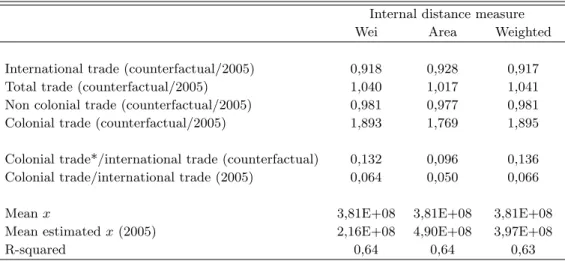
6. The results are qualitatively similar for all three measures of internal distance. We thus focus our discussion on the simplest measure, the Wei (1996) measure of internal distance. Predicted trade flows in 2005 exhibit a fairly good fit; when compared to the 25675 observations for which we actually have trade data, the R-squared is 0.64.25
Changing political borders affects both the volume and the geography of trade flows. Our results show that international trade, i.e. flows crossing a border, is 9% larger in 2005 than what it would have been with 1945 borders. The increase in the number of independent countries since WWII has led to a sizeable increase in measured international trade.
The picture is however different when we consider all trade flows, i.e. trade flows between the 181 countries for which data are available, irrespective of whether they cross a border or not. In 2005, all these countries are independent, so that all their trade flows are recorded as international trade. In our counterfactual world, 13% of trade takes place between regions of the same country or a colonizer and its colonies, and is not recorded as international trade. When all trade flows are considered, total trade in 2005 is 4% lower than what it would have been with 1945 borders. Increasing the number of independent countries therefore increases the measured international trade by increasing the number of flows recorded as international trade, but it reduces the volume of these flows by creating new border barriers.
As regards the geography of world trade, trade between former regions of the same country and between colonizers and their colonies in 2005 is half its value in our
counterfac-24German reunification is not taken into account here since Germany was divided into the Federal Republic of Germany and the German Democratic Republic in 1949.
25We calculate R-squared as the squared correlation between the observed and the predicted bilateral exports.
tual world. The presence of new border barriers between these countries also affects their exchanges with the rest of the world because it increases their average trade barriers. In the aggregate, former regions of the same country and colonizers and their colonies trade 1.9% more with third countries. A country’s break-up therefore affects third countries’ trade.
Finally, trade between OECD countries is only marginally affected by new political borders. France and the UK are exceptions since their bilateral trade is estimated to have increased by 2% thanks to the decolonization process. In the aggregate, French and English trade with the rest of OECD countries is 1% larger in 2005 than in our counterfactual world.
Table 6: Estimations of world trade in 2005 and in the counterfactual world
Internal distance measure
Wei Area Weighted
International trade (counterfactual/2005) 0,918 0,928 0,917 Total trade (counterfactual/2005) 1,040 1,017 1,041 Non colonial trade (counterfactual/2005) 0,981 0,977 0,981 Colonial trade (counterfactual/2005) 1,893 1,769 1,895 Colonial trade*/international trade (counterfactual) 0,132 0,096 0,136 Colonial trade/international trade (2005) 0,064 0,050 0,066
Mean x 3,81E+08 3,81E+08 3,81E+08
Mean estimated x (2005) 2,16E+08 4,90E+08 3,97E+08
R-squared 0,64 0,64 0,63
Notes: Computed from specification (1) in Table5for the Wei and area distance measures, and from specification (1) in Table7for the weighted distance measure.
*Trade between colonizers and their colonies and regions of the same country.
V
Conclusion
This paper investigates how the process of political break-up since World War II - the number of sovereign states has risen from 72 in 1948 to 192 today -, directly affects the volume and the geography of international trade. We first show that variation over time in the number of trade origins/partners recorded in international trade statistics create an accounting artefact in the measurement of world trade growth. Trade flows between regions of the same country in 1948 were indeed not recorded and, in the case of several colonies and countries, trade was simply not recorded in 1948. These discrepancies in the sample of countries included in the DOTS accounts for 17% of the growth in international trade between 1948 and 2007.
Second, we lay out an empirical strategy to investigate the impact of country break-ups on world trade based on a structural estimation of a gravity model of trade `a la
Anderson and van Wincoop (2003). We find that the rise in the number of independent countries since WWII has increased international trade by 9%, by raising the number of flows recorded as international trade, i.e. flows crossing a political border. It has however reduced total trade by 4%, i.e. including trade between former regions of the same country and former colonizers and their colonies, because new political borders create border barriers. Our results emphasize that the extensive margin of world trade related to the recognition of new sovereign states has a sizeable impact on the measurement of world trade growth since WWII. Our paper thus complements the results of Baier and Bergstrand (2001) on the determinants of the intensive margin of the growth in world trade.
This paper shows that the distribution of world GDP across sovereign political entities and their number matter for the measurement of trade openness. It suggests to be cautious when measuring trade globalization only by the trend in the trade to GDP ratio, without taking into account the number of potential trading partners in the world.
Appendix A
Table 7: Gravity results: weighted distance
(1) (2) (3)
X X > 0 log X
Estimator Poisson QML OLS
Current colonial relationship dum. 0.97c 0.90c 1.52a
(0.50) (0.49) (0.41) Ever in a colonial relationship 1.02a 0.99a 2.16a
or part of the same country dum. (0.09) (0.09) (0.09) Common colonizer dum. 0.06 0.06 0.71a
(0.13) (0.14) (0.07) Contiguity dum. 0.47a 0.47a 0.62a
(0.06) (0.06) (0.10) Log distance -0.89a -0.89a -1.75a
(0.04) (0.04) (0.03) Common language dum. 0.19a 0.19a 0.65a
(0.06) (0.06) (0.05) Common currency dum. -0.18b -0.18b -0.08
(0.08) (0.08) (0.13)
RTA dum. 0.30a 0.30a 0.21a
(0.07) (0.07) (0.05) WTO membership dum. 0.40b 0.46a 1.00a
(0.17) (0.17) (0.14)
Observations 29368 20289 20289
R-squared 0.92 0.92 0.73
Notes: a, b, c denotes significance at the 1, 5 and 10% level. Heteroscedasticity-robust standard errors are in parenthesis.
Appendix B
Table 8:Multilateral resistance terms Pσ−1in 2005 and in the
counterfactual world (CF)
Internal Distance Wei Area Weighted
Country CF 2005 2005/CF CF 2005 2005/CF CF 2005 2005/CF Belarus 19.6 26.7 1.36 15.3 24.3 1.59 26.7 36.8 1.38 Tajikistan 50.0 64.5 1.29 39.8 52.4 1.31 71.4 93.5 1.31 Kyrgyz Republic 39.8 51.0 1.28 31.0 40.2 1.30 56.8 73.5 1.29 Moldova 27.3 34.7 1.27 21.3 27.9 1.31 37.2 47.6 1.28 Georgia 27.9 35.3 1.27 22.1 30.8 1.39 38.9 48.8 1.25 Latvia 18.9 23.1 1.22 15.5 20.8 1.34 25.4 30.9 1.21 Namibia 49.0 59.9 1.22 36.5 51.3 1.41 75.2 89.3 1.19 Ukraine 19.2 23.5 1.22 16.7 24.8 1.48 26.7 32.8 1.23
Papua New Guinea 55.6 67.1 1.21 45.2 61.3 1.36 78.7 95.2 1.21
Azerbaijan 30.6 36.9 1.21 26.4 36.4 1.38 42.6 51.0 1.20 Marshall Islands 82.0 98.0 1.20 60.2 87.0 1.44 113.6 129.9 1.14 Estonia 19.7 23.5 1.19 15.9 20.8 1.31 26.2 31.1 1.18 Kazakhstan 32.3 38.5 1.19 28.5 39.8 1.40 47.2 56.2 1.19 Turkmenistan 46.9 55.9 1.19 40.5 50.5 1.25 68.0 80.6 1.19 Lithuania 16.9 20.1 1.19 14.7 19.4 1.32 22.5 26.7 1.18 Micronesia. Fed. Sts. 82.6 98.0 1.19 61.0 85.5 1.40 116.3 133.3 1.15 Palau 87.0 103.1 1.19 61.3 84.0 1.37 125.0 142.9 1.14 Uzbekistan 41.2 48.8 1.19 38.8 49.5 1.28 58.5 69.4 1.19 Armenia 30.7 36.2 1.18 26.7 33.4 1.25 41.5 49.0 1.18 Eritrea 73.0 85.5 1.17 56.8 67.1 1.18 108.7 128.2 1.18 Mauritania 65.8 74.1 1.13 48.1 55.6 1.16 100.0 112.4 1.12
Central African Republic 68.5 76.9 1.12 50.5 57.8 1.14 105.3 117.6 1.12
Niger 57.1 64.1 1.12 43.5 50.5 1.16 86.2 96.2 1.12
Bosnia and Herzegovina 32.1 35.7 1.11 31.4 36.0 1.14 43.3 48.5 1.12
Tunisia 21.3 23.7 1.11 19.7 23.8 1.21 28.7 31.8 1.11 Mali 56.5 62.5 1.11 45.5 52.6 1.16 84.7 93.5 1.10 Gambia. The 63.3 69.9 1.10 47.6 54.3 1.14 91.7 101.0 1.10 Sierra Leone 63.7 69.9 1.10 49.5 56.5 1.14 93.5 102.0 1.09 Chad 54.3 59.5 1.10 44.1 50.5 1.15 80.6 88.5 1.10 Djibouti 61.7 67.6 1.09 47.8 54.1 1.13 89.3 97.1 1.09 Algeria 26.2 28.7 1.09 26.4 31.6 1.20 37.3 41.0 1.10 Morocco 22.2 24.3 1.09 21.9 26.0 1.19 30.6 33.4 1.09 Guinea 55.9 61.0 1.09 46.1 52.6 1.14 81.3 88.5 1.09 Vanuatu 117.6 128.2 1.09 94.3 108.7 1.15 175.4 188.7 1.08 Sudan 48.3 52.6 1.09 48.3 55.6 1.15 71.4 77.5 1.09 Togo 53.8 58.5 1.09 46.1 52.4 1.14 76.9 82.6 1.07 Burkina Faso 49.5 53.8 1.09 43.5 49.8 1.14 71.4 76.9 1.08 Libya 34.1 36.9 1.08 35.2 41.8 1.19 48.8 52.6 1.08 Guyana 64.9 69.9 1.08 45.5 49.5 1.09 98.0 105.3 1.07 Benin 46.9 50.3 1.07 41.8 46.7 1.12 66.7 70.9 1.06 Dominica 57.8 61.7 1.07 45.5 49.8 1.09 78.7 82.6 1.05 Comoros 87.7 93.5 1.07 80.0 87.7 1.10 122.0 126.6 1.04 Senegal 43.3 46.1 1.06 42.7 48.5 1.14 60.6 64.1 1.06 Madagascar 66.2 70.4 1.06 61.0 67.6 1.11 97.1 102.0 1.05 Croatia 16.8 17.9 1.06 18.1 19.5 1.08 21.9 23.3 1.06 Gabon 46.5 49.3 1.06 45.9 50.8 1.11 65.8 69.4 1.06 Kiribati 137.0 144.9 1.06 106.4 114.9 1.08 204.1 212.8 1.04 Zimbabwe 60.6 64.1 1.06 50.3 54.1 1.08 88.5 92.6 1.05 Macedonia. FYR 28.5 30.0 1.05 25.4 26.7 1.05 38.0 40.0 1.05 Solomon Islands 102.0 107.5 1.05 75.2 81.3 1.08 153.8 161.3 1.05 Serbia 28.0 29.5 1.05 30.8 32.8 1.07 38.2 40.2 1.05 Belize 54.6 57.5 1.05 41.7 44.6 1.07 76.9 80.6 1.05
St. Kitts and Nevis 48.8 51.3 1.05 43.1 46.7 1.08 62.5 64.9 1.04
Lesotho 61.0 64.1 1.05 50.5 54.3 1.08 87.0 90.9 1.05 Malawi 60.6 63.7 1.05 54.3 59.2 1.09 86.2 90.1 1.05 Malta 17.3 18.2 1.05 19.5 21.8 1.12 20.7 21.6 1.04 Jordan 29.2 30.7 1.05 27.5 29.9 1.09 39.8 41.5 1.04 Cˆote d’Ivoire 38.9 40.8 1.05 41.7 46.1 1.11 54.3 56.8 1.05 Cameroon 38.5 40.3 1.05 38.6 42.2 1.09 54.3 56.8 1.05 St. Vincent 51.0 53.5 1.05 44.4 48.3 1.09 66.2 68.5 1.03 Ghana 41.7 43.7 1.05 41.5 45.2 1.09 58.1 60.6 1.04 Zambia 57.1 59.9 1.05 52.6 57.1 1.09 82.6 86.2 1.04 Grenada 48.5 50.8 1.05 43.7 47.4 1.09 62.1 64.1 1.03
Antigua and Barbuda 42.6 44.4 1.04 41.2 44.4 1.08 53.8 55.2 1.03
Slovenia 15.0 15.6 1.04 16.3 17.3 1.06 19.2 20.0 1.05
Internal Distance Wei Area Weighted Country CF 2005 2005/CF CF 2005 2005/CF CF 2005 2005/CF Slovak Republic 13.4 14.0 1.04 14.9 16.0 1.07 17.1 17.8 1.04 Uganda 46.1 48.1 1.04 46.1 50.0 1.09 64.5 67.1 1.04 Bhutan 80.6 84.0 1.04 61.3 64.9 1.06 123.5 128.2 1.04 St. Lucia 44.4 46.3 1.04 42.4 45.9 1.08 56.5 58.5 1.04 Tanzania 47.2 49.0 1.04 46.5 50.0 1.08 67.6 69.9 1.03 Seychelles 61.7 64.1 1.04 68.0 72.5 1.07 78.7 80.6 1.02 Philippines 19.0 19.7 1.04 24.3 27.4 1.13 25.7 26.5 1.03 Lao PDR 71.9 74.6 1.04 58.5 61.7 1.06 106.4 109.9 1.03 Lebanon 22.9 23.8 1.04 27.9 30.1 1.08 29.7 30.5 1.03 Swaziland 47.4 49.0 1.03 43.7 46.3 1.06 64.5 66.2 1.03 Tonga 109.9 113.6 1.03 105.3 111.1 1.06 149.3 151.5 1.02 Kenya 41.2 42.6 1.03 44.4 47.8 1.08 57.8 59.5 1.03 Cyprus 20.2 20.9 1.03 23.4 25.1 1.08 25.8 26.5 1.03 Russian Federation 13.5 13.9 1.03 24.8 26.1 1.05 19.3 20.0 1.03 Guinea-Bissau 80.6 83.3 1.03 59.5 61.7 1.04 122.0 126.6 1.04 Botswana 46.1 47.6 1.03 42.7 45.5 1.06 64.5 66.2 1.03
Syrian Arab Republic 26.7 27.5 1.03 34.1 37.0 1.09 35.8 36.9 1.03 Equatorial Guinea 45.5 46.9 1.03 53.2 56.5 1.06 61.3 62.9 1.03 Yemen. Rep. 51.5 53.2 1.03 55.6 58.8 1.06 74.1 75.8 1.02 Cambodia 50.0 51.5 1.03 47.4 50.3 1.06 69.9 71.4 1.02 Maldives 46.5 47.8 1.03 50.5 53.5 1.06 57.5 58.5 1.02 Jamaica 28.9 29.6 1.02 33.8 35.6 1.05 37.0 37.6 1.02 Congo. Rep. 22.9 23.4 1.02 43.1 47.4 1.10 27.4 27.8 1.01 Oman 28.2 28.9 1.02 32.8 34.2 1.04 38.5 39.1 1.02 Bangladesh 20.5 21.0 1.02 26.8 28.2 1.05 27.3 27.9 1.02 Pakistan 20.4 20.9 1.02 24.4 25.6 1.05 28.2 28.8 1.02 Fiji 55.9 57.1 1.02 62.9 66.2 1.05 73.5 74.6 1.01 Barbados 27.8 28.4 1.02 33.8 35.6 1.05 33.2 33.8 1.02 Nigeria 21.8 22.3 1.02 28.7 30.2 1.05 30.2 30.8 1.02 Samoa 108.7 111.1 1.02 105.3 109.9 1.04 147.1 149.3 1.01 Suriname 70.9 72.5 1.02 56.8 58.8 1.04 103.1 105.3 1.02
Trinidad and Tobago 21.5 21.8 1.02 28.2 29.3 1.04 26.7 27.0 1.01
Mauritius 28.1 28.6 1.02 37.9 39.4 1.04 34.4 34.7 1.01 Israel 10.1 10.3 1.02 14.4 14.9 1.04 12.8 12.9 1.01 Cape Verde 74.1 75.2 1.02 74.1 75.8 1.02 100.0 101.0 1.01 Czech Republic 11.6 11.7 1.01 13.6 13.9 1.02 15.0 15.2 1.01 Sri Lanka 27.6 28.0 1.01 35.8 37.0 1.03 36.4 36.8 1.01 Timor-Leste 129.9 131.6 1.01 108.7 109.9 1.01 192.3 192.3 1.00 Vietnam 31.3 31.7 1.01 41.2 42.4 1.03 43.5 43.9 1.01 Qatar 15.2 15.4 1.01 20.6 21.1 1.03 19.0 19.2 1.01 Brunei Darussalam 27.8 28.1 1.01 36.8 37.9 1.03 34.6 35.0 1.01 Rwanda 54.9 55.6 1.01 54.3 54.6 1.01 75.2 75.8 1.01 United Kingdom 4.2 4.2 1.01 6.5 6.7 1.02 5.5 5.6 1.01
Sao Tome and Principe 108.7 109.9 1.01 87.7 88.5 1.01 156.3 158.7 1.02
Bahrain 14.4 14.6 1.01 20.2 20.7 1.03 16.9 17.1 1.01
Kuwait 12.3 12.4 1.01 17.7 18.1 1.03 15.5 15.6 1.01
United Arab Emirates 13.4 13.6 1.01 19.3 19.8 1.02 17.5 17.6 1.01 Egypt. Arab Rep. 22.8 23.0 1.01 27.5 27.7 1.01 31.5 31.8 1.01
France 4.8 4.9 1.01 7.4 7.5 1.01 6.5 6.5 1.01 Angola 41.5 41.8 1.01 49.8 50.3 1.01 58.5 58.8 1.01 India 11.4 11.5 1.01 17.1 17.5 1.02 16.1 16.2 1.01 Burundi 74.1 74.6 1.01 62.5 63.3 1.01 105.3 106.4 1.01 Malaysia 17.2 17.3 1.01 24.7 25.1 1.02 23.1 23.3 1.00 Mongolia 67.1 67.6 1.01 47.4 47.4 1.00 102.0 102.0 1.00 Mozambique 51.0 51.3 1.01 54.9 55.2 1.01 70.4 70.4 1.00 South Africa 14.4 14.5 1.00 26.2 26.2 1.00 19.4 19.5 1.00
Hong Kong. China 5.3 5.3 1.00 8.6 8.6 1.01 6.1 6.1 1.00
Singapore 5.8 5.8 1.00 9.3 9.4 1.01 6.6 6.6 1.00
Congo. Dem. Rep. 21.9 22.0 1.00 51.8 51.8 1.00 26.0 26.0 1.00
Indonesia 17.5 17.5 1.00 26.5 26.6 1.01 24.3 24.3 1.00 Macao. China 9.5 9.5 1.00 14.7 14.7 1.00 10.2 10.2 1.00 Netherlands 5.4 5.4 1.00 8.1 8.1 1.00 6.9 6.9 1.00 Italy 5.0 5.0 1.00 7.9 7.9 1.00 6.6 6.6 1.00 United States 3.2 3.2 1.00 6.5 6.5 1.00 4.5 4.5 1.00 Argentina 15.3 15.3 1.00 31.9 31.9 1.00 20.5 20.5 1.00 Australia 15.5 15.5 1.00 24.9 24.9 1.00 22.2 22.2 1.00 Chile 21.8 21.8 1.00 31.0 30.9 1.00 29.9 29.9 1.00 China 8.3 8.3 1.00 14.3 14.2 1.00 11.8 11.8 1.00 Costa Rica 29.0 29.0 1.00 37.2 37.2 1.00 37.7 37.7 1.00 Dominican Republic 24.5 24.5 1.00 32.7 32.6 1.00 31.7 31.7 1.00 Haiti 45.7 45.7 1.00 46.3 45.9 0.99 60.6 60.6 1.00 Japan 3.4 3.4 1.00 5.8 5.8 1.00 4.5 4.5 1.00 Korea. Rep. 6.1 6.1 1.00 9.9 9.9 1.00 7.9 7.9 1.00 Nicaragua 51.8 51.8 1.00 48.3 48.1 1.00 71.4 71.4 1.00
Internal Distance Wei Area Weighted Country CF 2005 2005/CF CF 2005 2005/CF CF 2005 2005/CF New Zealand 19.6 19.6 1.00 30.5 30.4 1.00 26.0 26.0 1.00 Peru 28.1 28.1 1.00 37.2 37.0 1.00 39.1 39.1 1.00 Portugal 11.4 11.4 1.00 16.2 16.2 1.00 14.9 14.9 1.00 Paraguay 54.3 54.3 1.00 50.8 50.5 0.99 76.9 76.3 0.99 Uruguay 36.5 36.5 1.00 38.8 38.6 1.00 49.0 49.0 1.00 Germany 4.1 4.1 1.00 6.5 6.4 1.00 5.5 5.5 1.00 Spain 6.8 6.8 1.00 10.6 10.6 1.00 9.2 9.2 1.00 Switzerland 6.8 6.8 1.00 9.6 9.5 1.00 8.7 8.7 1.00 Canada 9.5 9.5 1.00 13.7 13.6 1.00 13.3 13.3 1.00 Greece 10.1 10.0 1.00 14.8 14.7 1.00 13.2 13.2 1.00 Ireland 10.2 10.2 1.00 14.0 13.9 0.99 13.2 13.2 1.00 Mexico 10.8 10.8 1.00 16.3 16.2 1.00 15.0 15.0 1.00 Sweden 11.0 11.0 1.00 15.3 15.3 1.00 14.8 14.8 1.00 Norway 11.2 11.2 1.00 15.6 15.5 0.99 15.0 15.0 1.00 Belgium 6.4 6.4 1.00 8.7 8.6 1.00 8.2 8.2 1.00 Austria 6.8 6.8 1.00 11.4 11.3 0.99 8.7 8.6 1.00 Brazil 13.7 13.6 1.00 21.4 21.4 1.00 19.6 19.6 1.00 Saudi Arabia 15.0 14.9 1.00 23.8 23.6 0.99 20.7 20.6 1.00 Denmark 8.2 8.2 1.00 11.5 11.5 1.00 10.5 10.4 1.00 Thailand 16.9 16.9 1.00 25.1 25.0 1.00 22.8 22.8 1.00 Finland 9.7 9.7 1.00 17.9 17.7 0.99 12.5 12.4 1.00 Venezuela. RB 20.1 20.1 1.00 28.0 27.9 1.00 27.6 27.6 1.00 Luxembourg 10.8 10.7 1.00 12.4 12.3 0.99 13.4 13.4 1.00 Poland 10.8 10.8 1.00 14.5 14.3 0.99 14.4 14.4 1.00 Turkey 11.0 10.9 1.00 16.1 16.0 1.00 14.9 14.9 1.00 Colombia 22.4 22.4 1.00 30.3 30.2 1.00 31.0 31.0 1.00 El Salvador 26.3 26.2 1.00 33.9 33.9 1.00 33.4 33.4 1.00 Hungary 13.4 13.4 1.00 16.9 16.7 0.99 17.5 17.5 1.00 Guatemala 28.0 27.9 1.00 34.5 34.4 1.00 37.0 37.0 1.00 Ecuador 29.4 29.3 1.00 37.3 37.2 1.00 39.5 39.5 1.00 Albania 31.0 30.9 1.00 31.1 30.7 0.99 41.2 40.8 0.99 Iceland 32.4 32.3 1.00 35.3 35.1 0.99 43.7 43.5 1.00 Romania 16.9 16.9 1.00 21.2 21.0 0.99 22.7 22.6 1.00 Panama 34.2 34.1 1.00 41.5 41.3 1.00 45.5 45.5 1.00 Honduras 41.8 41.7 1.00 44.6 44.4 1.00 56.2 56.2 1.00 Bulgaria 23.5 23.4 1.00 24.6 24.4 0.99 31.4 31.3 1.00
Iran. Islamic Rep. 23.5 23.4 1.00 33.1 32.9 0.99 33.3 33.2 1.00
Bolivia 56.2 55.9 0.99 51.5 51.3 0.99 80.6 80.6 1.00
Ethiopia 66.7 66.2 0.99 70.4 69.4 0.99 97.1 97.1 1.00
Nepal 43.1 42.7 0.99 41.8 41.3 0.99 59.5 59.2 0.99
Liberia 114.9 113.6 0.99 88.5 86.2 0.97 178.6 175.4 0.98
References
Alesina, A., Spolaore, E. and Wacziarg, R. (2000), “ Economic Integration and Political Disintegration ”, American Economic Review, vol. 90 no December: pp. 1276–
1296. 1
Anderson, J. E. and van Wincoop, E. (2003), “ Gravity with Gravitas: a Solution to the Border Puzzle ”, American Economic Review, vol. 93 no 1: pp. 170–192. 2,9,10,
11,14,16,20
Anderson, J. E. and van Wincoop, E. (2004), “ Trade Costs ”, Journal of Economic Literature, vol. XLII: pp. 691–751. 1
Baier, S. L. and Bergstrand, J. H. (2001), “ The growth of world trade: tariffs, transport costs, and income similarity ”, Journal of International Economics, vol. 53: pp. 1–27. 3,20
Estevadeordal, A., Frantz, B. and Taylor, A. M. (2003), “ The rise and the fall of world trade, 1870-1939 ”, The Quarterly Journal of Economics, vol. CXVIII no 2: pp. 359–407. 3
Feenstra, R. C. (2004), Advanced International Trade: Theory and Evidence, Princeton University Press, Princeton. 11
Felbermayr, G. J. and Kohler, W. (2006), “ Exploring the Intensive and Extensive Margins of World Trade ”, Review of World Economics (Weltwirtschaftliches Archiv), vol. 142 no 4: pp. 642–674. 6
Fidrmuc, J. and Fidrmuc, J. (2003), “ Disintegration and Trade ”, Review of Interna-tional Economics, vol. 11 no 5: pp. 811–829. 16
Frankel, J. A. (2008), “ The Estimated Effects of the Euro on Trade: Why Are They Be-low Historical Effects of Monetary Unions Among Smaller Countries? ”, NBER Working Papers 14542, National Bureau of Economic Research, Inc. 15
Gleditch, K. (2002), “ Expanded Trade and GDP Data ”, Journal of Conflict Resolution, vol. 46 no 5: pp. 712–274. 8
Glick, R. and Rose, A. K. (2002), “ Does a currency union affect trade? The time-series evidence ”, European Economic Review, vol. 46 no 6: pp. 1125–1151. 13
Head, K. and Mayer, T. (2002), “ Illusory Border Effects: Distance Mismeasurement Inflates Estimates of Home Bias in Trade ”, Working Papers 2002-01, CEPII research center. 16,17
Head, K., Mayer, T. and Ries, J. (2007), “ The erosion of colonial trade linkages after independence ”, Mimeo. 1,14,16
Helpman, E. (1987), “ Imperfect competition and international trade: Evidence from fourteen industrial countries ”, Journal of the Japanese and International Economies, vol. 1 no 1: pp. 62–81. 10,11
Hummels, D. (2007), “ Transportation Costs and International Trade in the Second Era of Globalization ”, Journal of Economic Perspectives, vol. 21 no 3. 1
Hummels, D., Ishii, J. and Yi, K.-M. (2001), “ The nature and growth of vertical specialization in world trade ”, Journal of International Economics, vol. 54 no 1: pp. 75–96. 1
Jacks, D. S., Meissner, C. M. and Novy, D. (2009), “ Trade Booms, Trade Busts, and Trade Costs ”, NBER Working Papers 15267, National Bureau of Economic Research, Inc. 3
Krugman, P. (1995), “ Growing World Trade: Causes and Consequences ”, Brookings Papers on Economic Activity, vol. 1: pp. 327–377. 1
McCallum, J. (1995), “ National Borders Matter: Canada-U.S. Regional Trade Pat-terns ”, American Economic Review, vol. 85 no 3: pp. 615–23. 2,14
Redding, S. and Venables, A. J. (2004), “ Economic geography and international in-equality ”, Journal of International Economics, vol. 62 no 1: pp. 53–82. 16
Rose, A. K. (1991), “ Why has trade grown facter than income? ”, Canadian Journal of Economics, vol. 24 no 2: pp. 417–427. 3
Rose, A. K. (2000), “ One money, one market: the effect of common currencies on trade ”, Economic Policy, vol. 15 no 30: pp. 7–46. 1,14,15
Russett, B. M., Singer, J. D. and Small, M. (1968), “ National Political Units in the Twentieth Century: A Standardized List ”, American Political Science Review, vol. 62 no 3: pp. 932–951. 4
Santos Silva, J. and Tenreyro, S. (2006), “ The Log of Gravity ”, Review of Economics and Statistics, vol. 88 no 4: pp. 641–658. 14
Small, M. and Singer, J. D. (1982), Resort to Arms: International and Civil Wars, 1816-1980, Sage Publications. 4
de Sousa, J. and Lamotte, O. (2007), “ Does political disintegration lead to trade disintegration? ”, The Economics of Transition, vol. 15: pp. 825–843. 1,16
Vicard, V. (2009), “ On Trade Creation and Regional Trade Agreements: Does Depth Matter? ”, Review of World Economics, vol. 145 no 2: pp. 167–187. 13
Wei, S.-J. (1996), “ Intra-National versus International Trade: How Stubborn are Nations in Global Integration? ”, NBER Working Papers 5531, National Bureau of Economic Research, Inc. 16,17,18
Documents de Travail
250. A. Monfort, «Une modélisation séquentielle de la VaR,» Septembre 2009
251. A. Monfort, “Optimal Portfolio Allocation under Asset and Surplus VaR Constraints,” September
2009
252. G. Cette and J. Lopez, “ICT Demand Behavior: An International Comparison,” September 2009 253. H. Pagès, “Bank Incentives and Optimal CDOs,” September 2009
254. S. Dubecq, B. Mojon and X. Ragot, “Fuzzy Capital Requirements, Risk-Shifting and the Risk Ta Channel of Monetary Policy,” October 2009
king
mpeting
a,”
cember 255. S. Frappa and J-S. Mésonnier, “The Housing Price Boom of the Late ’90s: Did Inflation Targeting
Matter?” October 2009
256. H. Fraisse, F. Kramarz and C. Prost, “Labor Court Inputs, Judicial Cases Outcomes and Labor Flows: Identifying Real EPL,” November 2009
257. H. Dixon, “A unified framework for understanding and comparing dynamic wage and price-setting models,” November 2009
258. J. Barthélemy, M. Marx and A. Poisssonnier, “Trends and Cycles: an Historical Review of the Euro Area,” November 2009
259. C. Bellégo and L. Ferrara, “Forecasting Euro-area recessions using time-varying binary response models for financial variables,” November 2009
260. G. Horny and M. Picchio, “Identification of lagged duration dependence in multiple-spell co risks models,” December 2009
261. J-P. Renne, “Frequency-domain analysis of debt service in a macro-finance model for the euro are December 2009
262. C. Célérier, “Forecasting inflation in France,” December 2009
263. V. Borgy, L. Clerc and J-P. Renne, “Asset-price boom-bust cycles and credit: what is the scope of macro-prudential regulation?,” December 2009
264. S. Dubecq and I. Ghattassi, “Consumption-Wealth Ratio and Housing Returns,” December 2009 265. J.-C. Bricongne, L. Fontagné, G. Gaulier, D. Taglioni and V. Vicard, “Firms and the Global Crisis:
French Exports in the Turmoil,” December 2009
266. L. Arrondel and F. Savignac, “Stockholding: Does housing wealth matter?,” December 2009 267. P. Antipa and R. Lecat, “The “housing bubble”and financial factors: Insights from a structural model
of the French and Spanish residential markets,” December 2009
268. L. Ferrara and O. Vigna, “Cyclical relationships between GDP and housing market in France: Facts and factors at play,” December 2009
269. L.J. Álvarez, G. Bulligan, A. Cabrero, L. Ferrara and H. Stahl, “Housing cycles in the major euro area countries,” December 2009
270. P. Antipa and C. Schalck, “Impact of Fiscal Policy on Residential Investment in France,” De 2009