Publisher’s version / Version de l'éditeur:
Wind & Structures, 8, May 3, pp. 213-233, 2005-05-01
READ THESE TERMS AND CONDITIONS CAREFULLY BEFORE USING THIS WEBSITE.
https://nrc-publications.canada.ca/eng/copyright
Vous avez des questions? Nous pouvons vous aider. Pour communiquer directement avec un auteur, consultez la première page de la revue dans laquelle son article a été publié afin de trouver ses coordonnées. Si vous n’arrivez pas à les repérer, communiquez avec nous à PublicationsArchive-ArchivesPublications@nrc-cnrc.gc.ca.
Questions? Contact the NRC Publications Archive team at
PublicationsArchive-ArchivesPublications@nrc-cnrc.gc.ca. If you wish to email the authors directly, please see the first page of the publication for their contact information.
NRC Publications Archive
Archives des publications du CNRC
This publication could be one of several versions: author’s original, accepted manuscript or the publisher’s version. / La version de cette publication peut être l’une des suivantes : la version prépublication de l’auteur, la version acceptée du manuscrit ou la version de l’éditeur.
Access and use of this website and the material on it are subject to the Terms and Conditions set forth at
Application of numerical models to evaluate wind uplift ratings of roofs.
Part II
Baskaran, B. A.; Molleti, S.
https://publications-cnrc.canada.ca/fra/droits
L’accès à ce site Web et l’utilisation de son contenu sont assujettis aux conditions présentées dans le site
LISEZ CES CONDITIONS ATTENTIVEMENT AVANT D’UTILISER CE SITE WEB.
NRC Publications Record / Notice d'Archives des publications de CNRC:
https://nrc-publications.canada.ca/eng/view/object/?id=deb9ae3d-761c-4ab5-b99f-3012bab9fde8 https://publications-cnrc.canada.ca/fra/voir/objet/?id=deb9ae3d-761c-4ab5-b99f-3012bab9fde8Application of numerical models to evaluate wind
uplift ratings of roofs: Part II
Baskaran, A.; Molleti, S.
NRCC-43935
A version of this document is published in / Une version de ce document se trouve dans :
Wind & Structures, v. 8, no. 3, May 2005, pp. 213-233
APPLICATION OF NUMERICAL MODELS TO
EVALUATE WIND UPLIFT RATINGS OF ROOFS
PART II
+ A. Baskaran1** and S. Molleti21
Senior Research Officer, National Research Council Canada,
Ottawa, Ontario, Canada, K1A 0R6
2
PhD Student,
Department of Civil Engineering, University of Ottawa, Ottawa, Ontario, Canada, K1N 6N5
ABSTRACT
Wind uplift rating of roofing systems is based on standardized test methods. Roof specimens are placed in an apparatus with a specified table size (length and width) then subjected to the required wind load cycle. Currently, there is no consensus on the table size to be used by these testing protocols in spite of the fact that the table size plays a significant role in wind uplift performance. Part I of this paper presented a study with the objective to investigate the impact of table size on the performance of roofing systems. To achieve this purpose, extensive numerical experiments using the finite element method have been conducted and benchmarked with results obtained from the experimental work. The present contribution is a continuation of the previous research and can be divided into two parts: (1) Undertake additional numerical simulations for wider membranes that were not addressed in the previous works. Due to the advancement in membrane technology, wider membranes are now available in the market and are used in commercial roofing practice as it reduces installation cost and (2) Formulate a logical step to combine and generalize over 400 numerical tests and experiments on various roofing configurations and develop correction factors such that it can be of practical use to determine the wind uplift resistance of roofs.
Key words:
Wind uplift, Roofing system, Test method, Numerical model, Thermoplastic, Thermoset, Modified bituminous, Fastener force and Correction factor.
+
Part I of the paper was published by the Journal of Wind and Structures, 4, (3), June 2001, pp. 213-226
**
1. Introduction
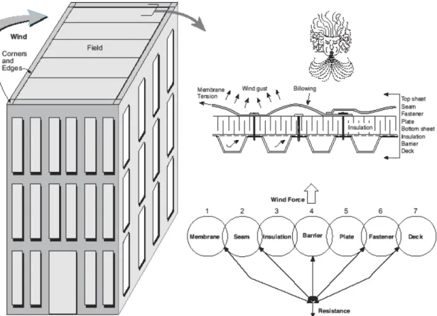
In North America, the membrane roofing systems can be classified in two categories based on the location of the roofing membrane. First, the inverted roofing system, where the membrane is covered by the insulation and other roof components and secondly, the conventional roofing system, where a flexible waterproof membrane is on the outer surface. In the latter the roofing membrane is exposed to external environmental conditions such as wind, snow, rain, UV and temperature changes. As shown in Figure 1 the flexible waterproof membrane is on the outer surface and attached to the deck at discrete points. Such roofing assemblies are known as Mechanically Attached roofing System (MAS). When subjected to wind dynamics, the MAS’s membrane flutters and deflects between the fastener rows. The MAS has several components and each component offers certain resistance to keep the system durable and sustaining the wind uplift force as illustrated through a force-resistance link diagram (Figure 1). All resistance links should remain connected. Failure occurs when wind uplift force is greater than the resistance of any one or more of these links.
Figure 1: Wind effects on single ply mechanically attached roof assemblies
In order to evaluate these force-resistance links, standardized methods have been developed {FM (Factory Mutual 1986), and UL Standard (Underwrites Laboratories 1991)}. In these test methods, the test specimen is assembled into a test frame as shown in Figure 2. Wind pressure, uniform with respect to space, is applied across the system until the system failure occurs. The system is considered to have failed when any one or more of the resistance links fail. Though the test specimen layout is similar to the field roof [e.g. the fastener row spacing (Fr), fastener spacing (Fs)] the aspect ratio of the test frame is normally smaller than that of the field roof. In lab conditions, the aspect ratio is defined as the length of the testing frame over width whereas in a field roof it can be the aspect ratio of the building. Due to this variation in the aspect ratio the measured response of the roofing system might be different from the field performance. When pressure is applied to the test specimen (Figure 2), the table edges offer some resistance thereby reducing the system responses such as fastener force and membrane deflection. This is a critical issue in the certification process of the roofing system. For example, testing a system with wider fastener row spacing in a narrow table can increase the influence of table edge effects on the system response. Alternatively, using a wider table for a system with narrow fastener spacing would slow down the system response. If the aspect ratio of the testing table is sufficient, then the roofing system response remains constant or minimum changes occur. Therefore an appropriate aspect ratio for the test table is necessary to obtain realistic wind uplift resistance.
Figure 2. Test frame nomenclature and components
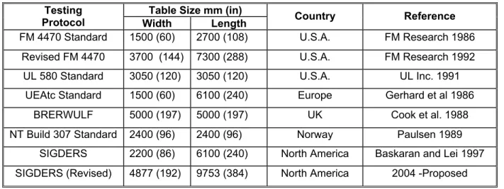
On the other hand, when reviewing the existing test methods, as grouped in Table 1, it is evident that tables with different aspect ratios are being used for the wind uplift evaluation of roofing systems. For instance, the FM (Factory Mutual 1986) tests use a table size of 1500 x 2700 mm (60” x 108”) or 3700 x 7300 mm (144” x 288”) depending on the roofing system. A chamber size of 3050 x 3050 mm (120” x 120”) is used by UL (Underwriters Laboratories 1991) standard. Present research efforts by a North American roofing consortium, the Special Interest Group for Dynamic Evaluation of Roofing Systems (SIGDERS) established at the National Research Council of Canada, have led to the development of a facility making it possible to evaluate roofing systems dynamically (Baskaran and Lei, 1997). A table size of 2200 x 6100 mm (86” x 240”) is used by the SIGDERS. For testing systems with wider membranes {systems with a membrane wider than 3050 mm (120”)}, a table size of 4880 x 9750 mm (192” x 384”) is proposed by the SIGDERS.
Table 1: Existing table sizes for certification of roofing systems
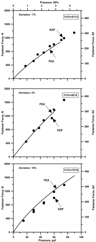
Despite the differences in the testing table aspect ratio and the significance of the edge effects on the roofing system performance, to the authors’ knowledge there is no existing criteria or standard to recommend a required table size for a specific system configuration. Therefore attempts have been made to address this issue using Finite Element (FE) modeling techniques. Numerical modeling can offer flexibility in exploring scenarios that would be too expensive or difficult to set up experimentally. In addition the analytical models are faster than the experimental approaches for solving problems where there is a need to investigate the impact of various influencing factors. The investigation of table size effect on wind uplift performance is an ideal example for such an application of numerical modeling. In the previous paper, the authors (Baskaran and Borujerdi, 2001) investigated the influence of table edges on the system response for three thermoplastic systems with a membrane width ranging from 1219 mm (48”) to 3048 mm (120”). The table edge effects were also investigated on systems by simulating 1000 mm (39”) wide modified bituminous membranes (Zaharai and Baskaran, 2001) and 1981 mm (78”) wide thermoset membrane (Borujerdi, 2004). Model validation and required table sizes were identified for the different system configurations (Fr/Fs) and correction factors were developed. Experimental data obtained from the DRF was used to benchmark the developed model. Average values of two characteristic parameters, i.e., fastener loads and membrane deflections measured from the DRF experiments were compared with the output of the FEA (Finite Element Analyses). Comparisons of fastener forces between the experimental and FEA modelling are shown in
Figure 3, in which the horizontal axis represents the applied suctions on the roof assembly and the vertical axis represents the fastener forces of the roofing systems response for the applied pressure. For the case of Fr/Fs = 67/12, an under-estimation of 7% by the FEA model
was found. Similar comparisons for the 48/18 and 72/18 configurations respectively revealed 2% and 10% deviations (over-estimations) of the analytical model from the measured fastener loads. These comparisons demonstrated that the FEA model is a viable tool that can be used to predict the fastener forces of test specimens at any uniform static pressure level.
Figure 3. Model validation for fastener forces. (after Baskaran and Borujerdi, 2001)
The present contribution is a continuation of the previous research and can be divided into two parts:
1. Undertake additional numerical simulations for wider membranes that were not addressed in the previous work. Due to the advancement in membrane technology, wider membranes are now available in the market and are used in commercial roofing practice as it reduces the installation cost.
2. Formulate a logical step to combine and generalize over 400 numerical tests and experiments on various roofing system configurations and develop correction factors such that it can be of practical use to determine the wind uplift resistance of roofs.
2. Numerical Modeling of Systems with Wider Membranes
Manufacturers, by taking advantage of the advancements in membrane technology, are introducing wider membranes into the roofing market. The introduction of wider membranes in both thermoplastic and thermoset groups and their extensive application in the field are the seed for the present investigation. Besides the field advantages and disadvantages of these wider membranes, efforts were not made to evaluate the table edge effects on the wind uplift performance of these wider membranes. Currently thermoplastic (thermoplastic olefin) membranes of 3658 mm (144”) wide and reinforced thermoset (ethylene propylene diene monomer) membranes of 3048 mm (120”) wide are available in the market. The present study focuses on the wind uplift performance of the systems with these wider membranes.
For the present study, a commercially available Finite Element program (ABAQUS version 6.3) with non-linear analysis capability was used to carry out all the numerical analysis. The large strains and deformations that occurred during the loading of the membrane were accounted for through geometrical non-linearity (large-displacements theory). Small load increments were considered to accommodate the flexibility of the membrane. As this study is
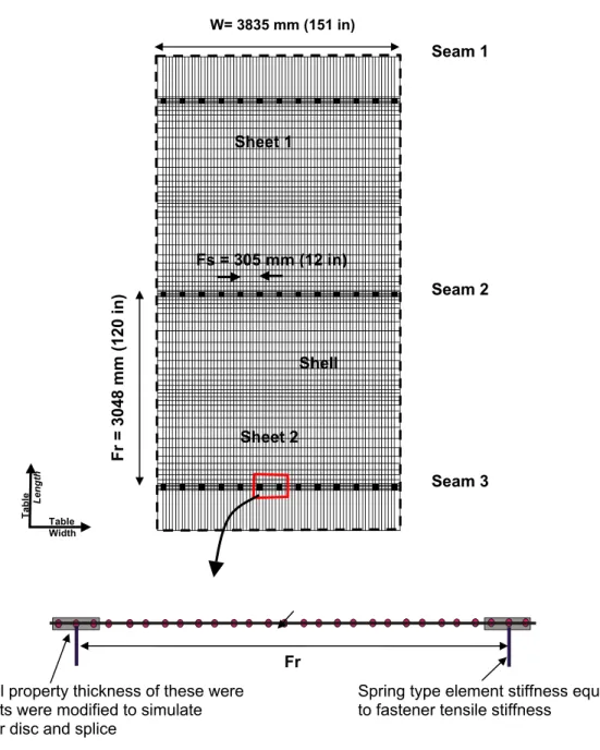
focused more on the behavior of the membrane with respect to the table width, only membrane deflections were considered in the numerical modeling. The deflections of the steel deck and insulation were assumed small in comparison to the membrane deflection. The thermoplastic membrane was simulated using a 4-node rectangular grid and shell elements were used to discretize the membrane (Figure 4). The element type was S4, which accounts for finite membrane strains and will allow for change in thickness. Shell elements of the membrane had a thickness of 1.04 mm (0.04”), and an equivalent modulus of elasticity of 300 MPa (43.5 ksi) and a Poisson ratio of 0.4. The modulus of elasticity and thickness of the membrane were obtained through mechanical tests in accordance to the ASTM standard (ASTM D 751-00 and ASTM D 6878-03).
Figure 4: FEM representation of thermoset system and seam details
Seam details were modeled by doubling the thickness of the shell element at the seam areas, 2.08 mm (0.08”) to simulate the spliced region of the membrane as schematically illustrated in Figure 4. Fasteners were modeled as spring supports with axial stiffness (vertical degree of freedom) of 20 N/mm (114 psi). The stiffness was extracted from the experimental results of force and displacement measurements of fasteners. The fastener plates were simulated as plastic discs by changing the material properties on the corresponding shell elements. These plastic plates were 3 mm (0.1”) thick with a diameter of 50 mm (2”) and a modulus of elasticity of 500 MPa (72.5 ksi).
As the seam area is subjected to high concentrated stresses, the aspect ratio of one was attained for the elements near the seam. In the model the membrane edges, i.e. the nodes along the perimeter of the membrane, as shown by the dotted lines in Figure 4, were restricted from any translation movement by fixing its three degrees (x, y, z) of freedom. The edge nodes have only rotational degrees of freedom (Φx, Φy, Φz ). To include the
large-displacement effects, the NLGEOM option was selected. Therefore most elements are formulated in the current configuration using current nodal position. The present study selected static stress analysis. This is found to be appropriate due to the fact that mass or inertia effects can be neglected. The analysis can be linear or non-linear and time-dependent effects of the membrane can be neglected however the rate-dependent plasticity is taken into account. The loading conditions are defined in the model by assuming a uniform static uplift pressure of 1.44 KPa (30 psf) on the membrane.
A similar approach was used for systems with thermoset membranes. However, shell elements had a thickness of 1.1 mm (0.043”) and an equivalent modulus of elasticity of 150 MPa (22 ksi) and a Poisson ratio of 0.22. Seam details were modeled by doubling the
thickness of the shell element at the seam areas, 2.2 mm (0.086”). Fasteners were modeled as spring supports with axial stiffness (vertical degree of freedom) of 60 N/mm (345 psi). The fastener plates were simulated as metal plates with a thickness of 2 mm (0.08”).
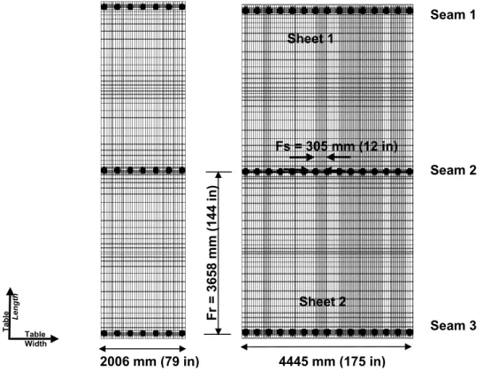
For the thermoplastic systems, simulations were performed for two configurations 3658 mm/305 mm (144”/12”) and 3658 mm/610 mm (144”/24”). For the remainder of the paper, set arrangements of this nature will be referred to as configuration 144/12 and configuration 144/24. The first number in the pair represents the fastener row spacing and the second number accounts for the fastener spacing and both are expressed as inch unit. Figure 5 gives an example of two simulated table widths. Both simulated tables had three rows of fasteners with 7 fasteners in each row in the case of the 2006 mm (79”) wide table and 15 fasteners for that of the 4445 mm (175”) wide.
Figure 5: FEM representation of 144/12 thermoplastic system on two different table widths
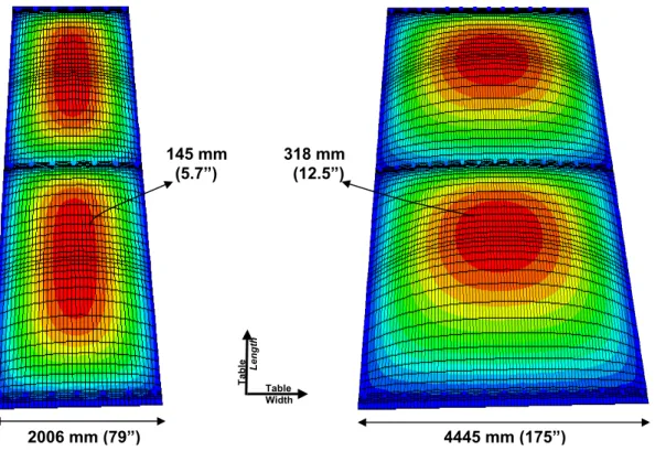
One of the advantages of the numerical modeling is the possibility to visualize and analyze the impact of these various influencing parameters. Figure 6 (a) and (b) clearly show the influence of the table edges on the membrane behavior for a thermoplastic system. The deflection of the membrane is a combination of the lateral deflection (i.e. between the table edges along the length (TEL)) and longitudinal deflection (i.e. between the fastener rows). For table widths less than the fastener row spacing (Fr) or membrane width (Figure 6(a)), the deflection of the membrane is laterally restricted by the table edges. The orientation of the membrane deflection is between the fastener rows thereby indirectly affecting the fastener forces along the seam with the middle fastener having the maximum fastener force. When the table width is greater than the Fr, the orientation of the membrane deflection changes along the length (TEL) and due to the greater membrane width and less influence of the table edges the deflection of the membrane increases (Figure 6(b)). The elongated shape of the middle contour along the table width indicates that the middle fastener and its adjacent fasteners may have similar fastener force.
Figure 6(a): Contour plot of the membrane deflection for 144/12 thermoplastic system on a 2006 mm (79”) table
Figure 6 (b): Contour plot of the membrane deflection for 144/12 thermoplastic systems on a 4445 mm (175”) table
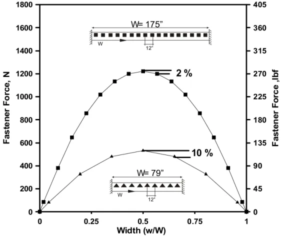
To demonstrate this observation, the resulting fastener forces (along the middle seam or seam 2) are plotted in Figure 7 with respect to the normalized table width. Computed results indicated that on a 4445 mm (175”) table, three fasteners along the seam have similar
fastener force with a variation of 2%, as compared to the 2006 mm (79”) table where the middle fastener force varies by 10% from the adjacent ones. This reveals the edge influence on the fastener force on the 2006 mm (79”) table while it is negligible on the 4445 mm (175”) table.
Figure 7: Fastener force variation along the seam for 144/12 thermoplastic systems on 2006 mm (79”) and (4445 mm) 175” tables
3. Required Table Width for Systems with Wider Membranes
This section focuses on the determination of the ideal table size for the systems with wider membranes. As shown in Figure 2, all the three dimensions, namely length, width and depth, constitute the table size. Components used in the lab experiments are similar to those used in the field. In other words, there is no variation in the thickness of components such as insulation and membrane. Therefore, the depth was not considered in the analysis. The effect of table length is minimal because during the system installation, membrane width forms parallel to the table width. However, the table length effect was numerically investigated and it was concluded (Borujerdi, 2004) that the minimum length of the table should be greater than twice the sheet width so that the table length can have a minimum of three seams with the middle seam or seam 2 (Figure 4) positioned symmetrical to the table length and free from the influence of table edges (TEW).
The present investigation focuses to isolate the effect of table width effect on the system response using the validated FE model. With all other parameters maintained constant, the Required Table Width (RTW) is one that will provide a roofing system response in the lab similar to that of the field. Moreover, the development of the RTW requires several levels of generalization of the true wind-induced effect over a roof assembly. Often, these generalizations warrant compromise from the technically sound approach to the practically acceptable procedure. This research work had the luxury of receiving input from all parties concerned with roofing, including researchers, manufacturers, roofing associations representing the contractors, and building owners (refer to the acknowledgment section for the SIGDERS consortium participants). Based on the numerical investigation and the practical inputs the following criteria were established to identify the RTW:
“The table with RTW should provide no change in the maximum fastener forces or change in the maximum fastener force should be within 5% compared to those obtained while decreasing the table width by 305 mm (12”)”.
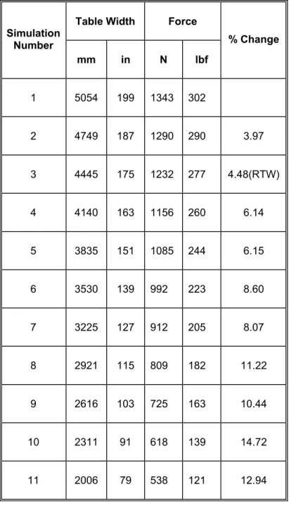
For each configuration, to determine the RTW simulations a table width of 2006 mm (79”) was used at the start and incremented by 305 mm (12”). For each simulated table width, a suction pressure of 30 psf (1.44 KPa) was applied. The computed fastener force from the middle fastener along seam 2 and the deflection at the mid-span of the membrane between two fastener rows were obtained. For illustrating the above-mentioned criteria of the RTW and involved calculations, a typical example is shown in Table 2. Table 2 presents the computed maximum fastener forces for the configuration of 144/12. A computed fastener force of 1343 N (302 lbf) was calculated for a table width of 5054 mm (199”). By decreasing the table width to 4445 mm (175”), the fastener force was decreased to 1232 N (277 lbf). Further reduction of the table width reduces the fastener force. For a table width of 2006 mm (79”), the computed fastener force was only 538 N (121 lbf). This reduction from 1343 N (302 lbf) to 538 N (121 lbf) is due to the greater influence of the table edges on the 2006 mm (79”) table width when compared to the 5054 mm (199”) table width. By applying the established criteria of the RTW, a table width of 4445 mm (175”) can be selected as the RTW. Similar calculations were done for the configuration of 144/24 and a 5054 mm (199”) table width was determined as the RTW.
Table 2: Determining the RTW for 144/12 thermoplastic system
For thermoset system with EPDM membrane, the simulations were performed for three configurations, namely, 120/12, 120/18 and 120/24. The RTW was determined for each configuration by modeling table widths starting from 2006 mm (79”) and incrementing by 305 mm (12”). Also, a suction pressure of 1.44 KPa (30 psf) was applied for all the simulated table widths and the fastener force and the deflection data were obtained. The procedure, similar to the one discussed for Table 2, was followed for the determination of the RTW. The RTW for the investigated configurations is as follows:
Configuration: 120/12; RTW = 3835 mm (151”) Configuration: 120/18; RTW = 3835 mm (151”) Configuration: 120/24; RTW = 4140 mm (163”)
A number of parameters can influence the RTW, in particular fastener spacing (Fs), fastener row spacing (Fr) and membrane properties.
4. Correction Factor for Systems with Wider Membranes
In the previous section the RTW’s were established for thermoplastic and thermoset systems with wider membranes. If any of these system configurations are tested on a table narrower than the established RTW, then the measured fastener load is not necessarily suitable as the design fastener load. Due to the narrow table width, the boundary or edge effects can reduce
the load transferred to the fasteners during the experimental measurement. This load can be adjusted or corrected by applying a correction factor to obtain the design fastener load for that system. The correction factor can be calculated by dividing the fastener force obtained from the RTW with that of the narrow one as illustrated in Table 3. Tables having larger widths than the RTW have a correction factor equal to one.
Table 3: Example to illustrate the development of correction factors
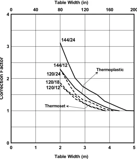
In total, 22 simulations were performed on the thermoplastic system on two configurations, 144/12 and 144/24. For each configuration, correction factors were developed and the correction factor curves are plotted as shown in Figure 8, in which the horizontal axis represents the table width and the vertical axis represents the correction factors. Similarly, in the case of the thermoset system, 27 simulations were performed on three configurations, 120/12, 120/18 and 120/24. The developed correction factor curves are also included in Figure 8. As it can be seen, the thermoset system configurations of 120/12 and 120/18 have the same RTW of 3835 mm (151”).
Figure 8: Developed correction factors for systems with wider membranes These plotted data clearly revealed that wider membranes require wider tables. For the proper evaluation of the wind uplift resistance of these wider membranes, testing has to be done on the appropriate wider tables such that their wind uplift performance is least affected by table edges thereby determining the actual wind uplift loads. It is worth recalling that none of the existing testing organizations, as grouped in Table 1, is appropriate to investigate such wide membranes without the application of the correction factors.
5. Generalization of Correction Factors for Roofing Design
The intent of this present study is to achieve characteristic correction factor curves such that guidelines can be developed for the general roofing system design. To achieve this objective, the previous work done by the authors was summarized and combined with the present study on wider membranes as follows:
For the thermoplastic system, data from Baskaran and Borujerdi, 2001 (Figure 9) and wider membrane data from the present study (Figure 8) were combined.
For the thermoset system, data from Borujerdi, 2004 (Figure 10) and wider membrane data from the present study (Figure 8) were combined.
For the modified bituminous system, data from Zaharai and Baskaran, 2001 (Figure 11) were used.
Figure 9: Developed correction factors for thermoplastic systems (Baskaran and Borujerdi, 2001)
Figure 10: Developed correction factors for thermoset systems (Borujerdi, 2004) Figure 11: Developed correction factors for mod-bit systems (Zaharai and Baskaran,
2001)
Table 4 summarizes all the simulations performed for the different system configurations to form a database. In total, 372 numerical tests were combined with 20 benchmark experiments to provide a wide range database. The fifth column in Table 4 indicates the number of data set for each configuration. For example, configuration 6 on thermoplastic system with fastener row spacing of 1701 mm and fastener spacing of 305 mm has 15 numerical data (simulations from 76 to 90) by covering a range of table widths from 787 to 5054 mm. It also has 6 experimental data (experiments from 3 to 8) for variation in the test protocol and repetitive experiments.
Table 4: Data Base used for the generalization of correction factors
To generalize the developed correction factor, attempts have been made to identify a relationship between the correction factor and the influencing parameters (Fr, Fs and W).
Using the data sets from Table 4, three parameters were calculated. Those values consist of a ratio of:
Fastener row spacing to fastener spacing (Fr/Fs) – labeled as m
Table width to fastener spacing (W/Fs) – labeled as n
Table width to fastener row spacing (W/Fr) – labeled as k
For a configuration, m indicates the number of fasteners for that configuration. When this configuration is tested on a table width W, n gives the number of fasteners for that table. Based on this analogy, a relationship between m and n is developed for further analysis of the data. Table 5 shows an example of the developed relationship between m, n and CF for
the thermoplastic roofing system in tabular format showing examples for m as 2, 5.6 and 12. It is clear that for the table with RTW, n > m. Also, a correction factor has to be applied to account for the edge effect when n < m.
First, the trend of systematically decreasing the correction factor becomes clear for each set of m. Then the table was grouped based on m ratio. In doing so, the 30 different configurations were reduced to 21 (Figures 8 to 11). It was owing to the fact some configurations such as 72/18 and 48/12 had the same m ratio of four. Then, the data sets in
each category were sorted in descending order according to correction factor values. It was noticed the n and k ratios increased in each data sets when the correction factor decreased.
Table 5. Parameter normalization for correction factor – thermoplastic system
To investigate the underlying relationship further, a normalization procedure was applied for all configurations grouped in the database (Table 4). A total of 8 characteristic curves were generated. These characteristic curves are shown in Figure 12 with an n value on the x-axis and a correction factor on the y-axis. Comparison of these curves revealed the following points:
1. Characteristic curves can be grouped into four sets based on the following relationship:
Set 1: m < 2.0 Set 2: 2 = m < 3.5 Set 3: 3.5 = m < 7 Set 4: m > 7
2. In the computed data n ranges from 1 to 20, which has the corresponding correction factors of 4.0 and 1.0 respectively. This indicates that a table width of 12192 mm (480’’) can be sufficient to evaluate any system configurations without the application of correction factors. This forecast is based on the maximum value of the x-axis value for Set 4 and calculated as follows:
Maximum x-axis value from Figure 12 = 20
n = 20
W/Fs = 20
W = 20 Fs
Taking the maximum fastener spacing {Fs = 610 mm (24”)} used in the industry, W = 20 X 24 = 480” (12192 mm).
3. For a given constant value of m, increasing the n reduces the correction factor. It also reveals that the ratio of n increases while the table width increases and causes the correction factor to reduce when systems are tested on a wider table.
4. For a constant value of n, the correction factor has a direct relation with m. In other words, the correction factor increases while m increases. For instance, for a value of n = eight (Set 4 in Figure 12), the values of the correction factor increase linearly from 1.4 to 1.8 while m increases from 8 to 12. This provides the option to interpolate values between m-curves.
Based on the above analysis, it can be concluded that no correction factor is needed or correction factor is equal 1.0, if:
m < 2 as n > 5 m < 3 as n > 10 m < 7 as n > 15 m < 12 as n > 20
This is evident from Figure 12 as the value of the x-axis for Set 2, Set 3 and Set 4 can be obtained by multiplying the Set 1 x-axis value using 2, 3 and 4 respectively. Although the correction factors (Figure 12) cover a wide range of table widths, the factors may not be practical for some cases. Displayed data of Set 1 clearly shows a minimum value of n as 4 on the x-axis. Note that the n shows the number of fasteners along the table. This means that a minimum table width should be greater than 3 times the fastener spacing. For example, when the width of the table decreases to 787 mm (31”), the table cannot be used for the evaluation of a system with a fastener spacing of the 610 mm (24”). For particular application, Set 1 can be excluded. Also, the higher correction factors create accumulative errors for the measured fastener force. Therefore, it has been decided to set a maximum of 1.5 for the correction factor. In other words, the measured fastener force can be corrected only as much as twice to get the design fastener force. Based on this extensive data analysis, Figure 13 shows the generalized correction factor for the roofing system design. One can apply interpolation to obtain correction factors for m values that are not shown in Figure 13. The following section illustrates two practical scenarios for the application correction factors.
Figure 13: Generalized correction factor curves for roofing design
6. Application of the Generalized Correction Factor Curves
For a given system configuration, the m-curve intercept with the x-axis of Figure 13 gives the RTW. Systems tested with RTW or greater table widths are exempted from the application of the correction factor (i.e. the influences of table edges on the measured fastener force are minimum). Systems tested in all other tables that are less than RTW, the y-axis gives the correction factors. Using these correction factors, one can obtain the design fastener force. To illustrate the involved process, a case study is shown as follows:
Scenario 1: A proponent tested a flexible membrane roof system with fastener row
spacing of 1829 mm (72”) and a fastener spacing of 305 mm (12”) using a table width of 2743 mm (108”). Experimentally measured fastener force was 1300 N (295 lbf).
Step 1: Calculate m and n m = Fr/Fs
= 72/12 = 6
n = W/Fs
= 108/12
= 9
Step 2: Identify correction factor
For the values of 6 and 9, Figure 13 gives a correction factor of 1.00. Step 3: Calculate design fastener force
This implies that the measured fastener force is not affected by the table edges. Therefore the design fastener force is the same as the measured fastener force of 1300 N (295 lbf).
Scenario 2: A membrane with fastener row spacing of 2743 mm (108”) was tested in
the same table with the same fastener spacing. Experimentally measured fastener force was 1700 N (382 lbf).
Step 1: Calculate m and n m = Fr/Fs = 108/12 = 9 n = W/Fs = 108/12 = 9
Step 2: Identify correction factor
Interpolating the curves for the ratio of m = 8 and 10, Figure 13 gives a correction factor of 1.32.
Step 3: Calculate design fastener force
Design fastener force = Measured fastener x Correction factor = 1700 x 1.32 = 2244 N (510 lbf)
7. Concluding Remarks
Applying a finite element based model, numerical experiments were performed on mechanically attached systems with thermoset, thermoplastic and modified bituminous membranes. Using the benchmarked model for each system, different configurations were investigated to identify the effect of table width on the system response. An increase in the table width beyond a certain size did not significantly change the system response. It is termed as the required table width and it depends on the system configuration. For each system configuration, correction factors were developed such that they can be used in a
situation where the testing table is less than the required table width. The developed correction factors for all systems were combined and generalized to form design curves that can be of practical use to determine the wind loading on roofs. Nevertheless, the both discussed numerical model and experimental approaches are limited to uniform pressure distribution over the roof assembly. The model has the potential to simulate the spatial pressure variation over the roof assembly that really occurs in full scale. On going research efforts on this topic will be the focus of a future paper.
References
ABAQUS (2002), User’s manual, Hibbitt, Karlsson & Sorensen, Inc., Pawtucket, RI. USA. ASTM standard ASTM D 6878-03, Standard Specification for Thermoplastic Polyolefin Based
Sheet Roofing, Annual Book of ASTM Standards, American Society for Testing and Materials, Philadelphia, PA.
ASTM standard, ASTM D 751-00, Tensile Test is done using Procedure B-Cut Strip Test Method, Annual Book of ASTM Standards, American Society for Testing and Materials, Philadelphia, PA
Baskaran, A., Borujerdi, J., 2001. Application of numerical models to determine wind uplifts ratings of roofs. Wind & Structures, an International Journal, Vol. 4, No. 3 (2001), 213-226.
Baskaran, A., Lei, W. & Richardson, C. 1999. Dynamic Evaluation of Thermoplastic Roofing Systems for Wind Performance. Journal of Architectural Engineering, ASCE, Vol. 5, No 5, pp 16-24.
Baskaran, A. & Lei, W. 1997. A New Facility for Dynamic Wind Performance Evaluation of Roofing Systems. Proceedings of the Fourth International Symposium on Roofing
Technology, NRCA/NIST, Washington, D.C., U.S.A., pp. 168-179.
Borujerdi, J., 2004. Numerical Evaluation of Low Slope Roof for Wind Uplift, Master of Applied Sciences, Department of Civil Engineering, University of Ottawa, ON, Canada. Cook, N.J., Keevil, A.P. & Stobart, R.K. 1988. BRERWULF- The Big Bad Wolf. Journal of
Wind Engineering and Industrial Aerodynamics. Vol. 29, pp. 99-107.
Factory Mutual Research, 1986. Approval Standard (5 by 9): Class I Roof Covers (4470), Norwood, Massachusetts, USA.
Factory Mutual Research, 1992. Approval Standard (12 by 24): Class I Roof Covers (4470), Norwood, Massachusetts, USA.
Gerhardt, H.J. & Kramer, C. 1986. Wind Induced Loading Cycle and Fatigue Testing of Lightweight Roofing Fixations. Journal of Wind Engineering and Industrial Aerodynamics, Vol. 23, pp. 237-247.
Paulsen, E.M. 1989. NBI Roof Wind Uplift Strength Test Facility and Load Programs.
Proceedings of the Roof Wind Uplift Testing Workshop, Oak Ridge, Tennessee, pp.
46-51.
Underwriters Laboratories Inc. 1991. Standard for Wind Uplift Pressure of Roof Assemblies (UL 580). Third edition, Nov. 1991.
Zahrai, S.M., Baskaran, A. 2001. Table size effect on wind resistance of modified bituminous roofing systems, International Conference on Building Envelope Systems and
Acknowledgement
The presented research is being carried out for a consortium - Special Interest Group for Dynamic Evaluation of Roofing Systems (SIGDERS). SIGDERS was formed from a group of partners who were interested in roofing design. These partners included:
Manufacturers
Atlas Roofing Corporation, Canadian General Tower Ltd., Carlisle Syntec Incorporated, GAF Materials Corporation, GenFlex Roofing Systems, Firestone Building Products Co., IKO Industries Ltd., ITW Buildex, Johns Manville, Sarnafil, Soprema Canada and Stevens Roofing Systems, Tremco Inc and Trufast Corporation
Building Owners
Canada Post Corporation, Department of National Defence, Public Works and Government Services Canada.
Industry Associations
Canadian Roofing Contractors' Association, Canadian Sheet Steel Building Institute, Industrial Risk Insurers, National Roofing Contractors’ Association and Roof Consultants Institute.
Memb rane Insula tion Deck
L
W
Table Edges Bottom Frame Top Chamber W L Membrane FastenersL = Table Length TEL = Table edges along the length Fr = Fastener row spacing W = Table width TEW = Table edges along the width Fs = Fastener spacing
Table 1: Existing table sizes for certification of roofing systems Table Size mm (in)
Testing
Protocol Width Length Country Reference
FM 4470 Standard 1500 (60) 2700 (108) U.S.A. FM Research 1986 Revised FM 4470 3700 (144) 7300 (288) U.S.A. FM Research 1992
UL 580 Standard 3050 (120) 3050 (120) U.S.A. UL Inc. 1991 UEAtc Standard 1500 (60) 6100 (240) Europe Gerhard et al 1986
BRERWULF 5000 (197) 5000 (197) UK Cook et al. 1988
NT Build 307 Standard 2400 (96) 2400 (96) Norway Paulsen 1989 SIGDERS 2200 (86) 6100 (240) North America Baskaran and Lei 1997 SIGDERS (Revised) 4877 (192) 9753 (384) North America 2004 -Proposed
FEA 0 400 800 1200 1600 2000 F a st en er F o rc e , N Fr/Fs=67/12 EXP 0 1 2 3 4 0 100 200 300 400 Pressure, KPa Fa st ene r Fo rce , lb f Deviation: -7% 0 400 800 1200 1600 2000 F a st en e r F o rce , N Fr/Fs=48/18 EXP FEA 0 100 200 300 400 Fa st ene r Fo rce , lb f Deviation: 2% 0 20 40 60 80 100 0 400 800 1200 1600 2000 Fa stene r F o rc e, N Fr/Fs=72/18 Pressure, psf EXP FEA 0 100 200 300 400 Fast ener Force, lb f Deviation: 10%
W= 3835 mm (151 in) Table Width Table Length Shell Fr
Spring type element stiffness equals to fastener tensile stiffness
Material property thickness of these were elements were modified to simulate fastener disc and splice
Seam 3 Seam 2 Seam 1 Sheet 2 Sheet 1 Fs = 305 mm (12 in) Fr = 304 8 mm (1 20 in)
Table Width Table Length 2006 mm (79 in) Seam 3 Seam 2 Seam 1 Sheet 2 Sheet 1 Fs = 305 mm (12 in) Fr = 365 8 mm (1 44 in) 4445 mm (175 in)
318 mm (12.5”) 145 mm (5.7”) 4445 mm (175”) 2006 mm (79”) Table Width Table Length
Figure 6(a): Contour plot of the membrane deflection for 144/12 thermoplastic system on a 2006 mm (79”) table
Figure 6 (b): Contour plot of the membrane deflection for 144/12 thermoplastic system on a 4445 mm (175”) table
0 0.25 0.5 0.75 1 Width (w/W) 0 200 400 600 800 1000 1200 1400 1600 1800 F a st en e r Fo rce, N 0 45 90 135 180 225 270 315 360 405 Fa s te ne r Fo rce , lb f
2 %
10 %
W 12”W= 79”
12” WW= 175”
Figure 7: Fastener force variation along the seam for 144/12 thermoplastic systems on 2006 mm (79”) and (4445 mm) 175” tables
Table 2: Determining the RTW for 144/12 thermoplastic system
Table Width Force
Simulation Number mm in N lbf % Change 1 5054 199 1343 302 2 4749 187 1290 290 3.97 3 4445 175 1232 277 4.48(RTW) 4 4140 163 1156 260 6.14 5 3835 151 1085 244 6.15 6 3530 139 992 223 8.60 7 3225 127 912 205 8.07 8 2921 115 809 182 11.22 9 2616 103 725 163 10.44 10 2311 91 618 139 14.72 11 2006 79 538 121 12.94
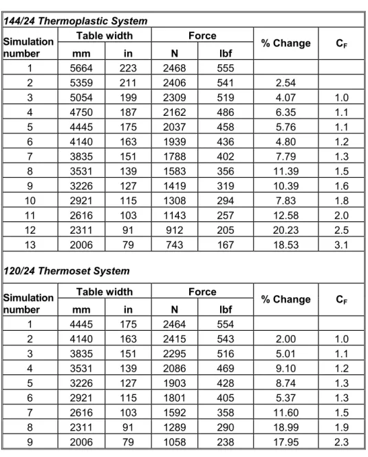
Table 3: Example to illustrate the development of correction factors 144/24 Thermoplastic System
Table width Force
Simulation number mm in N lbf % Change CF 1 5664 223 2468 555 2 5359 211 2406 541 2.54 3 5054 199 2309 519 4.07 1.0 4 4750 187 2162 486 6.35 1.1 5 4445 175 2037 458 5.76 1.1 6 4140 163 1939 436 4.80 1.2 7 3835 151 1788 402 7.79 1.3 8 3531 139 1583 356 11.39 1.5 9 3226 127 1419 319 10.39 1.6 10 2921 115 1308 294 7.83 1.8 11 2616 103 1143 257 12.58 2.0 12 2311 91 912 205 20.23 2.5 13 2006 79 743 167 18.53 3.1 120/24 Thermoset System
Table width Force
Simulation number mm in N lbf % Change CF 1 4445 175 2464 554 2 4140 163 2415 543 2.00 1.0 3 3835 151 2295 516 5.01 1.1 4 3531 139 2086 469 9.10 1.2 5 3226 127 1903 428 8.74 1.3 6 2921 115 1801 405 5.37 1.3 7 2616 103 1592 358 11.60 1.5 8 2311 91 1289 290 18.99 1.9 9 2006 79 1058 238 17.95 2.3
0 1 2 3 4 5 Table Width (m) 0 1 2 3 4 C o rr e c ti o n Fa c to r 0 40 80 120 160 200
Table Width (in)
144/24 144/12 120/24 120/18 120/12 Thermoplastic Thermoset
0 1 2 3 4 5 0 1 2 3 4 Co rr ec ti on F a c to r 0 40 80 120 160 200
W, Table Width (in)
48/6 48/12 48/18 48/24 0 1 2 3 4 5 0 1 2 3 4 0 40 80 120 160 200
W, Table Width (in)
67/6 67/12 67/18 67/24 0 1 2 3 4 5 Table Width (m) 0 1 2 3 4 Co rr e c ti on Fa c to r 0 40 80 120 160 200
W, Table Width (in)
72/6 72/12 72/18 72/24 0 1 2 3 4 5 Table Width (m) 0 1 2 3 40 40 80 120 160 200 114/12 114/18
0 1 2 3 4 5 Table width,m 0 1 2 3 4 Co rr e c ti on Fa c to r 0 40 80 120 160 200 Table Width,in 78/18 78/12 78/6
Figure 10: Developed correction factors for thermoset systems (Borujerdi, 2004)
0 1 2 3 4 5 Table Width,m 0 1 2 3 4 Co rr ec ti o n F a c to r 0 40 80 120 160 200 Table Width, in Group # 1 : 35/6-35/24 Group # 2 : 35/6-35/24
Table 4: Data Base used for the generalization of correction factors Thermoplastic Systems Configuration Fr* (mm) Fs* (mm) Table Width (W) range (mm)* # of Simulations # of Experiments 1 (48/6) 1219 152 787 – 5054 1-15 2 (48/12) 1219 305 787 – 5054 16-30 3 (48/18) 1219 457 787 – 5054 31-45 1-2 4 (48/24) 1219 610 787 – 5054 46-60 5 (67/6) 1701 152 787 – 5054 61-75 6 (67/12) 1701 305 787 – 5054 76-90 3-8 7 (67/18) 1701 457 787 – 5054 91-105 8 (67/24) 1701 610 787 – 5054 106-120 9 (72/6) 1829 152 787 – 5054 121-135 10 (72/12) 1829 305 787 – 5054 136-150 11 (72/18) 1829 457 787 – 5054 151-165 9-10 12 (72/24) 1829 610 787 – 5054 166-180 13 (114/12) 2896 305 787 – 5054 181-195 14 (114/18) 2896 457 787 – 5054 196-210 15 (144/12) 3658 305 2006 – 5054 211-221 16 (144/24) 3658 610 2006 – 5664 222-234
Modified bituminous Systems: Group # 1 1 (35/6) 890 152 787 – 4140 1-12
2 (35/12) 890 305 787 – 4140 13-24 11-14
3 (35/18) 890 457 787 – 4140 25-36 4 (35/24) 890 610 787 – 4140 37-48
Modified bituminous Systems: Group # 2
5 (35/6) 890 152 787 – 4140 49-60 6 (35/12) 890 305 787 – 4140 61-72 7 (35/18) 890 457 787 – 4140 73-84 15-16 8 (35/24) 890 610 787 – 4140 85-96 Thermoset Systems 1 (78/6) 1981 152 2006 – 3225 1-5 17-18 2 (78/12) 1981 305 2006 – 3225 6-10 19-20 3 (78/18) 1981 457 2006 – 3225 11-15 4 (120/12) 3048 305 2006 – 4445 16-24 5 (120/18) 3048 457 2006 – 4445 25-33 6 (120/24) 3048 610 2006 – 4445 34-42 372 20
Table 5: Parameter normalization for correction factor – thermoplastic system
W
mm (in) mm (in) Fr mm (in) Fs Cf K = r
F
W
n = sF
W
m = s rF
F
1086 (43) 1220 (48) 610 (24) 4.025 0.9 1.8 2 1390 (55) 1220 (48) 610 (24) 2.405 1.1 2.3 2 1695 (67) 1220 (48) 610 (24) 1.706 1.4 2.8 2 2000 (79) 1220 (48) 610 (24) 1.353 1.6 3.3 2 2305 (91) 1220 (48) 610 (24) 1.166 1.9 3.8 2 2610 (103) 1220 (48) 610 (24) 1.062 2.1 4.3 2 2914 (115) 1220 (48) 610 (24) 1 2.4 4.8 2 …. …. …. …. …. …. …. …. …. …. …. …. …. …. 781 (31) 1700 (67) 305 (12) 3.683 0.5 2.6 5.6 1086 (43) 1700 (67) 305 (12) 2.464 0.6 3.6 5.6 1390 (55) 1700 (67) 305 (12) 1.877 0.8 4.6 5.6 1695 (67) 1700 (67) 305 (12) 1.505 1 5.6 5.6 2000 (79) 1700 (67) 305 (12) 1.285 1.2 6.6 5.6 2305 (91) 1700 (67) 305 (12) 1.144 1.4 7.6 5.6 2610 (103) 1700 (67) 305 (12) 1.057 1.5 8.6 5.6 2914 (115) 1700 (67) 305 (12) 1 1.7 9.6 5.6 …. …. …. …. …. …. …. …. …. …. …. …. …. 781 (31) 1830 (72) 152 (6) 2.921 0.4 5.2 12 1086 (43) 1830 (72) 152 (6) 2.120 0.6 7.2 12 1390 (55) 1830 (72) 152 (6) 1.634 0.8 9.2 12 1695 (67) 1830 (72) 152 (6) 1.344 0.9 11.2 12 2000 (79) 1830 (72) 152 (6) 1.170 1.1 13.2 12 2305 (91) 1830 (72) 152 (6) 1.063 1.3 15.2 12 2610 (103) 1830 (72) 152 (6) 1 1.4 17.2 122 4 6 8 1 2 3 4 2 = m < 2.5 2.5 = m < 3.5 Set 2 m = 2 m = 3 3 6 9 12 15 n 1 2 3 4 Co rr e c ti on F a c to r 3.5 = m < 4.5 4.5 = m < 7 Set 3 m = 4 m = 6 1 2 3 4 5 1 2 3 4 C o rr e c ti o n f a c to r m < 2 m = 1 Set 1 4 8 12 16 20 n 1 2 3 4 7 = m < 8.5 8.5 = m < 10.5 10.5 = m < 13 Set 4 m = 8 m = 10 m = 12 10
3 5 7 9 11 13 15 17 n = W / Fs 1.00 1.05 1.10 1.15 1.20 1.25 1.30 1.35 1.40 1.45 1.50 Co rr ect io n F act o r, C F m= 2 m= 3 m= 4 m= 6 m= 8 m= 10 m= 12 m = Fr / Fs