Publisher’s version / Version de l'éditeur:
Vous avez des questions? Nous pouvons vous aider. Pour communiquer directement avec un auteur, consultez la
première page de la revue dans laquelle son article a été publié afin de trouver ses coordonnées. Si vous n’arrivez pas à les repérer, communiquez avec nous à [email protected].
Questions? Contact the NRC Publications Archive team at
[email protected]. If you wish to email the authors directly, please see the first page of the publication for their contact information.
https://publications-cnrc.canada.ca/fra/droits
L’accès à ce site Web et l’utilisation de son contenu sont assujettis aux conditions présentées dans le site LISEZ CES CONDITIONS ATTENTIVEMENT AVANT D’UTILISER CE SITE WEB.
Student Report (National Research Council of Canada. Institute for Ocean Technology); no. SR-2008-06, 2008
READ THESE TERMS AND CONDITIONS CAREFULLY BEFORE USING THIS WEBSITE. https://nrc-publications.canada.ca/eng/copyright
NRC Publications Archive Record / Notice des Archives des publications du CNRC :
https://nrc-publications.canada.ca/eng/view/object/?id=ccb8c9d2-4eb0-4449-8391-aa852e1a93f0 https://publications-cnrc.canada.ca/fra/voir/objet/?id=ccb8c9d2-4eb0-4449-8391-aa852e1a93f0
NRC Publications Archive
Archives des publications du CNRC
For the publisher’s version, please access the DOI link below./ Pour consulter la version de l’éditeur, utilisez le lien DOI ci-dessous.
https://doi.org/10.4224/8896280
Access and use of this website and the material on it are subject to the Terms and Conditions set forth at A remote icing thickness measurement system
National Research Council Canada Institute for Ocean Technology Conseil national de recherches Canada Institut des technologies oc ´eaniques
Student Report
SR-2008-06
A Remote Icing Thickness Measurement System
M. Pham
April 2008
DOCUMENTATION PAGE
REPORT NUMBER
SR-2008-06
NRC REPORT NUMBER DATE
April 2008 REPORT SECURITY CLASSIFICATION
Unclassified
DISTRIBUTION
Unlimited TITLE
A REMOTE ICING THICKNESS MEASUREMENT SYSTEM
AUTHOR(S)
Mark Pham
CORPORATE AUTHOR(S)/PERFORMING AGENCY(S)
Institute For Ocean Technology - National Research Council of Canada PUBLICATION
N/A
SPONSORING AGENCY(S)
Institute For Ocean Technology - National Research Council of Canada IOT PROJECT NUMBER NRC FILE NUMBER
KEY WORDS Ice detector PAGES 19, App. A FIGS. 30 TABLES SUMMARY
A description on the apparatus, theory and test results on the ice detection system.
ADDRESS National Research Council Institute for Ocean Technology Arctic Avenue, P. O. Box 12093 St. John's, NL A1B 3T5
National Research Council Conseil national de recherches
Canada Canada
Institute for Ocean Institut des technologies Technology océaniques
A REMOTE ICING THICKNESS MEASUREMENT SYSTEM
SR-2008-06
Mark Pham
Table of Contents:
1.0 Introduction... 3
2.0 Theory – Glaze Ice... 4
3.0 Theory – Rime Ice ... 5
4.0 Apparatus ... 8 4.1 The Laser ... 8 4.2 The Detector... 9 4.3 Wiring ... 10 4.3.1 The Laser ... 11 4.3.2 The Detector... 12 5.0 Computer Software ... 12
5.1 Pan Tilt Remote (PTR) ... 13
5.2 ZoomBrowser ... 13
5.3 Remote Foggy Icing Thickness Sensor (RFITS) ... 13
6.0 Manual (Method for Icing Measurement)... 14
7.0 Testing... 17
7.1 Testing Setup Description... 17
7.2 Summary of Testing Performed... 18
7.3 Summary of Testing Results... 19
8.0 Conclusion ... 19
Table of Figures
Fig. 1: The setup of the system ...Error! Bookmark not defined. Fig. 2: The detector ...Error! Bookmark not defined. Fig. 3: The laser ...Error! Bookmark not defined. Fig. 4: Appearance of laser beam on clear ice ...Error! Bookmark not defined. Fig. 5: Total internal reflection of light in clear ice ...Error! Bookmark not defined. Fig. 6: Light diffraction in translucent ice ...Error! Bookmark not defined. Fig. 7: Photo of laser beam on translucent ice ...Error! Bookmark not defined. Fig. 8: Diagram showing pertinent angles ...Error! Bookmark not defined. Fig. 9: A view of a skewed ellipse due to pan and tilt ...Error! Bookmark not defined. Fig. 11: Diagram showing the rotational angle RV of the detector, RV Error! Bookmark
not defined.
Fig. 12: Diagram showing the rotational angle of the laser, RL... Error! Bookmark not
defined.
Fig. 13: Separation distance between the centers ...Error! Bookmark not defined. Fig. 14: Servo for laser focus...Error! Bookmark not defined. Fig. 15: Control box for filter and the focus of the laser and telescope..Error! Bookmark
not defined.
Fig. 16: Optical zoom camera mounted on laser ...Error! Bookmark not defined. Fig. 17: Monitor of the optical zoom camera ...Error! Bookmark not defined. Fig. 18: The detector apparatus, camera and telescope ...Error! Bookmark not defined.
Fig. 19: The servo to control the focus of the telescope ....Error! Bookmark not defined. Fig. 20: The potentiometers that are calibrated to give readings of the pan and tilt angles
...Error! Bookmark not defined. Fig. 21: Screenshot of ZoomBrowser start-up menu ...Error! Bookmark not defined. Fig. 22: Icon to begin remote shooting in ZoomBrowser..Error! Bookmark not defined. Fig. 23: Select directory for saved images...Error! Bookmark not defined. Fig 24: Screenshot of remote shooting in ZoomBrowser ..Error! Bookmark not defined. Fig 25: Screenshot view of the RFITS program ...Error! Bookmark not defined. Fig 26: Photographs of apparatus setup in the model prep shop area...Error! Bookmark
not defined.
Fig. 27: Fresh water was frozen onto a lifeboat hook...Error! Bookmark not defined. Fig. 28: Aluminium block that was used to melt the icing at a control rate ... Error!
Bookmark not defined.
Fig. 29: Graph 1, shows the relation between measured vs. actual for all points... Error!
Bookmark not defined.
Fig 30: Graph 2, shows the correlation between measured vs. actual but excluding the measurements for 12 and 13 strips...Error! Bookmark not defined.
Appendices:
Appendix A: Diagram of wiring setup for the ice detector
Appendix B: Remote Foggy Icing Thickness Sensor’s programming code Appendix C: Calibration Equations for potentiometers and pixels to millimetres Appendix D: Data from Testing
Appendix E: Pictures and Data for each measurement Appendix F: Diagram of Circuit Board
1.0 Introduction
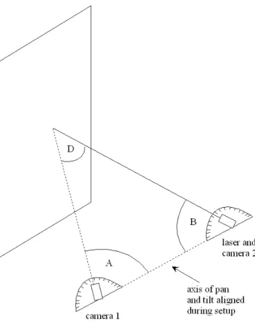
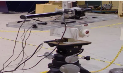
Dr. Robert Gagnon, Institute of Ocean Technology has designed and developed a system for detection and measurement of layers of icing build-up on marine ships, aircrafts and space shuttles. The ice detector was designed to accurately give measurements of the thickness of the layer of ice using a remote system (non-contact) using a laser and a detector (see fig. 1-3), which consists of camera and image analysis software. A remote system is often required in situations where it would be dangerous to run wires near any materials that are flammable or explosive. A significant feature of the ice detector is its ability to detect both types of ice, rime and glaze, which accumulate on a surface of space shuttles and airplanes. The machine is able to measure ice thickness at different locations on a surface without requiring relocating or reconfiguring the device. The only adjustment that needs to be made in order to detect at a different location, on a surface, is to point the laser and the camera in the direction of the new location. This remote system is an efficient and accurate solution to measuring the thickness of the different types of ice over a surface.
The research and development of the ice detector will provide great benefits to the space and aviation industry to ensure the safety and performance of their respective crafts under icy conditions. Icing build-up on space shuttles and airplanes poses dangerous hazards due to the reduce performance causing unexpected behaviour or component failures of the craft which causes disastrous results.
2.0 Theory – Glaze Ice
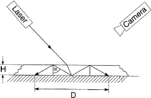
The two types of icing build-up that can accumulate onto a surface are glaze ice and rime ice. Since there are multiple types of ice, different methods must be used in order to calculate the thickness of the layer. The apparatus used in both types are the same; however, the difference occurs in the appearance of the refracted, scattered light after it strikes the surface. In order to measure the thickness of either type of icing build-up, a laser is directed at the ice surface of interest and a detector is used to photograph a picture of that particular area so that a computer program can analyze the photo and return the thickness measurement. In the case of glaze ice, the two features of interest are a bright spot that is surrounded by a dark circle or ellipse. The bright spot is due to the laser beam initially hitting the top layer of the ice surface. The dark circle that surrounds this bright spot occurs due to the total internal reflection, which occurs because as light travels through medium of higher refractive index, ice, to a medium with a lower refractive index, air, the light is unable to escape back out therefore causing a dark circle (see fig. 4 and 5). The diameter of this dark circle is proportionally related to the thickness of the ice and is calculated using the following formula:
) ( * 4 Tan α D
H
=
(Eqn. 1)where H is the thickness of the ice, D is the diameter of the dark circle and α is the critical angle of reflected beam and can be found using the following equation:
⎟ ⎠ ⎞ ⎜ ⎝ ⎛ = − n 1 sin 1 α (Eqn. 2)
where n is the refractive index of the medium. For ice, α is approximately equal to 50 degrees. The requirement for measuring glaze ice is sim ple; one would only need to know the diameter of the dark circle in order to calculate the thickness using the two equations above.
3.0 Theory – Rime Ice
In order to measure the thickness of rime ice, a different method has been developed in order to account for the differences in the behaviour of the light beam as it passes through the ice surface. When light strikes the ice layer, it produces an initial point, spot 1, on the top surface of the ice and as the light refracts and scatters, it produces a light blob (see fig. 6 and fig. 7). The distance that separates the center of the blob of light and the center of the initial bright spot as it strikes the surface will be used to calculate the thickness of the ice.
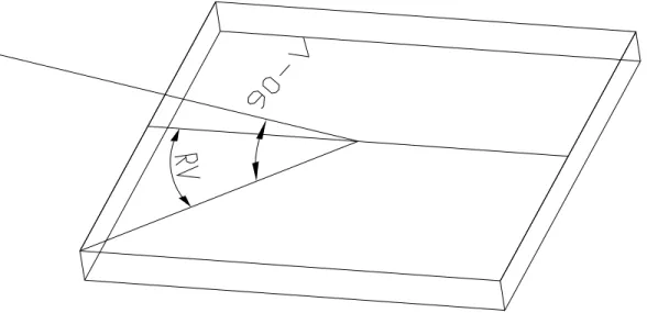
Certain measurements are required to measure the thickness of rime ice, these measurements are the pan and tilt of the laser and camera and the range, which is the distance from the camera to the surface. The pan and tilt of the camera and laser are used to calculate the values A and B (see fig. 1) using the following equation:
(
)
(
)
⎥ ⎥ ⎥ ⎥ ⎥ ⎦ ⎤ ⎢ ⎢ ⎢ ⎢ ⎢ ⎣ ⎡ ⎥ ⎦ ⎤ ⎢ ⎣ ⎡ ⎟⎟ ⎠ ⎞ ⎜⎜ ⎝ ⎛ − − − = − − ) 90 sin( ) tan( tan cos cos * ) 90 sin( cos 90 1 1 camerapan cameratilt cameratilt camerapan A (Eqn. 3) and(
)
(
)
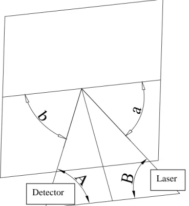
⎥ ⎥ ⎥ ⎥ ⎥ ⎦ ⎤ ⎢ ⎢ ⎢ ⎢ ⎢ ⎣ ⎡ ⎥ ⎦ ⎤ ⎢ ⎣ ⎡ ⎟⎟ ⎠ ⎞ ⎜⎜ ⎝ ⎛ − − − = − − ) 90 sin( ) tan( tan cos cos * ) 90 sin( cos 90 1 1 laserpan lasertilt lasertilt laserpan B (Eqn. 4)After determining A and B, we can solve for angles a, the angle of the laser beam to the surface, and b, the angle of the view to the surface (see fig. 8), from the equations:
B A b a+ = + (Eqn. 5) and
E
D
b a=
) sin( ) sin( (Eqn. 6)where D is the height of the laser beam and E is the horizontal distance that through the center of the ellipse (see fig. 9). After solving for angles a and b, the incidence angles of the laser, L, the camera, V and the tilt of the plane, T, which are measured from the normal of the surface (see fig. 5 and 10), can be calculated using the following formulas:
(
)
⎥⎥⎦ ⎤ ⎢ ⎢ ⎣ ⎡ + − = − 2 1 ) sin( ) tan( 1 ) cos( ) tan( tan 90 T a T a L (Eqn. 7) and(
)
⎥⎥⎦ ⎤ ⎢ ⎢ ⎣ ⎡ + − = − 2 1 ) sin( ) tan( 1 ) cos( ) tan( tan 90 T b T b V (Eqn. 8) and ⎥ ⎦ ⎤ ⎢ ⎣ ⎡ + = − ) sin( ) sin( tan 1 b a D a M TAfter determining the two incident angles and the tilt angle, the rotational angles of the camera, RV, and the laser, RL, are shown, respectively, in fig. 11 and 12. These angles can be computed using the following equations:
)) sin( ) (tan( tan 1 b T RV = − (Eqn. 9) and )) sin( ) (tan( tan 1 a T RL= − (Eqn. 10)
The last two angles that needs to be computed are the refraction angles of the view, AV, and the laser, AL, these are determined by solving for:
) / ) (sin( sin 1 V n AV = − (Eqn. 11) and ) / ) (sin( sin 1 L n AL= − (Eqn. 12) where n is refractive index of the ice. Now that all the necessary angles have been defined and the thickness, h, of the ice can be calculated by the following equation:
⎥ ⎦ ⎤ ⎢ ⎣ ⎡ + = ) tan( ) cos( ) tan( ) cos( 1 ) tan( ) cos( ) sin( AV RV AL RL AV RV b S H (Eqn. 13)
where S is the horizontal separation between the center of the bright spot on the surface
and the centre of the light blob (see fig. 13).
The required measurements needed to calculate the thickness of the ice are the pan and
spot on the surface and the light blob and the range, which is the distance from the
camera to the surface. The range along with the focal length and zoom ratio, which is
data that is automatically stored after each individual photo is taken, are used to adjust the
size of the image from the photo to the equivalent actual size on the surface.
4.0 Apparatus
The following section will give a description of the two major components, the laser and the detector, of the ice detection system (as shown in fig. 2 and 3) and its function in the process of determining the ice thickness.
4.1 The Laser
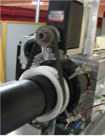
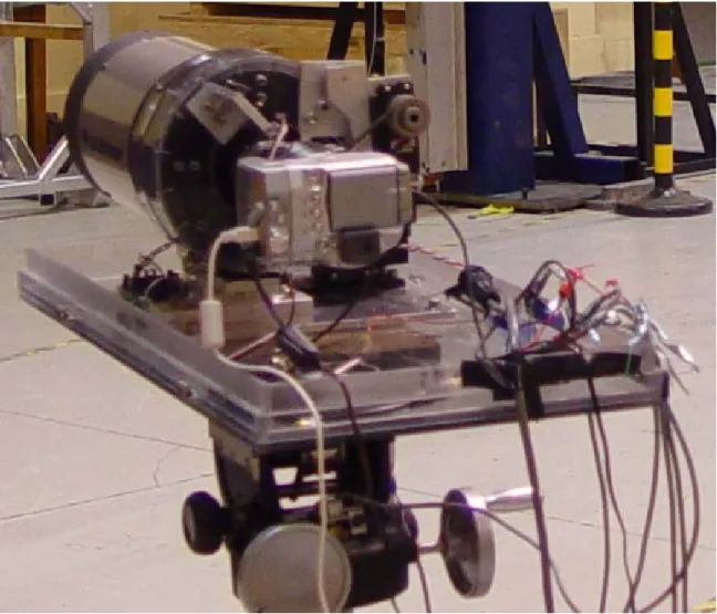
The first of the two major components is the laser. The laser that is being used in this project is a 15 mW Melles Griot model. The focus dial on the laser can be adjusted through the system of three pulleys, a trapezoidal-toothed timing belt and a winch servo (see fig. 14). One pulley is attached to the dial and the second pulley is connected to the servo. The last remaining pulley is located on the opposite side of the servo and it is used to reduce the load on the laser. The user is able to control the servo from a distance by using a controller (fig. 15) to rotate the dial to adjust the focus. In order for the controller to see in the direction that the laser is pointing towards, an optical zoom camera was mounted onto the base plate (see fig. 16). The camera is connected to a monitor (see fig.17) and a controller to allow the operator to view and zoom in or out to achieve a better view of the surface.
The entire base plate is situated on top of a Quickset motor control that allows the user to control the pan and tilt of the machine from a distance away using the Pan Tilt Remote (PTR) software. This device also has the added benefit that it automatically feeds back the pan and tilt angles to allow for the Remote Foggy Icing Thickness Sensor (RFITS) software to calculate thickness of the icing build-up. The motor control and the base plate are mounted on top of a tripod as a form of stable support.
4.2 The Detector
The other major component is the detector. It is composed of a telescope and a digital camera (see fig. 18). The telescope that is use in the development process is a Schmidt-Cassegrain Optical Celestron CS telescope; it is mounted onto a base plate. In certain lighting conditions, a light filter is required. This filter is controlled by a wing servo. The wing servo only has the capability to rotate 90 degrees so an extension was attached to allow for the wing servo the ability to rotate even further to be able to attach and remove the filter properly so that it does not obstruct the view through the telescope. Two pulleys, a timing belt and a servo are attached to the focus dial on the telescope to allow the user to control the focus of the telescope using the controller box (see fig.4), also, a potentiometer is attached to the focus dial to measured the range (see fig. 19), the distance from the camera to the surface. A Canon camera is mounted onto the eyepiece of the telescope. This allows photos to be taken with the ZoomBrowser program by the controller situated at the computer.
In the situation where weather may pose to be a problem, the laser and the detector can be encased in a lexan housing with a window that can be opened or closed to ensure that the casing is not affecting the measurements.
The entire detector system is mounted onto a tripod. The base is equipped with a potentiometer that is calibrated to give an accurate reading on how many degrees the pan and tilt angles have been changed (see fig. 20).
A computer is connected to both the laser and the detector system. The computer, using specialized software, is then able to compute the thickness of the layer of ice from the known variables of pan and tilt angles, distance between the centers of the initial bright spot on the ice and the center of the refracted blob of light and the range.
4.3 Wiring
The electrical wiring of the detector and the laser is another important aspect of the assembly of the ice detector. In the following sections, each of the major components’ electrical wiring will be discussed in detail. A schematic diagram of the entire wiring process is included in appendix A.
4.3.1 The Laser
The motor control, the device that controls the pan and tilt of the laser, uses a serial cable in order for the computer software to control the device and read the angles measurements output. The output signal of the motor control is also necessary for the ice detection program, RFITS, in order to get the required measurements of the pan and tilt angles from the laser for calculating the thickness of the ice. In order to get this information, a terminal block was incorporated into the wiring in order for a second serial wire to tap into this output signal. Both, the cable for the motor control and the cable that taps into the signal, were converted from serial cables to USB wires using an adaptor. These cables then are connected to one of two USB hubs to eliminate the need for multiple wires by converting the two USB cables into one Ethernet cable by using an USB extender, which is a device that allows the signal to travel over a long distance that would not be capable otherwise. The Ethernet cable that runs from one USB extender near the laser to another USB extender near controller. This signal is now converted back to a USB wire, which can be directly plugged into the laptop.
The optical zoom camera that is mounted on the base plate has two wires that run from the camera to a monitor and a controller. One of the wires is the video cable that is connected to the monitor is to allow the user to see the view of the camera. The second cable that is connected to the camera controls the zoom feature; this allows the user to zoom in or out to get a better view of where the laser is pointing.
The last remaining wires that spans from the laser to the controller box are used to control the servo, which is used to adjust the focus on the laser.
4.3.2 The Detector
The wiring for the detector is straightforward. The camera that is attached to the telescope has a USB cable that connects to the second USB hub near the detector system. This wire allows for the camera software, ZoomBrowser, to view and photograph pictures from a distance location.
The three potentiometers that are attached to the tripod, to determine the pan, tilt and range, each has their own separate analog wire. These wires are connected to an analog-to-digital converter, thereby reducing the three analog wires into just one USB cable. This cable is then connected to the same USB hub as the camera where an USB extender is used to convert the USB cable to an Ethernet cable to transmit the data to another USB extender where the wire can be converted back into an USB cable to connect the laptop. The advantage of using two USB extender to change the wiring from an USB cable to an Ethernet cable is the ability to run the wires a longer distance, thus allowing the person controlling the device to be far away from apparatus.
5.0 Computer Software
The icing measurement system uses three programs in order to calculate the thickness of the build-up of ice on the surface. Two of the three programs, Pan Tilt Remote (PTR) and ZoomBrowser, are used to control the different devices, the Quickset motor control and
the camera respectively, from a distance. The last program, Remote Foggy Icing Thickness Sensor (RFITS), is used to calculate the thickness based on the different input information gathered by the sensors and potentiometers.
5.1 Pan Tilt Remote (PTR)
The PTR program is used to control the Quickset motor control that is attached to the tripod. The program is capable of moving the base plate, in the horizontal and vertical plane by using the crosshair function, so that the laser can point at the exact area where icing build-up measurement is required. PTR continuously feeds back information regarding the pan and tilt angles of the laser and this data is used to calculate the thickness. PTR also has a function that can move the laser’s base plate to its physical center; this is useful in initial zeroing of the pan and tilt angles.
5.2 ZoomBrowser
ZoomBrowser is a program that is associated with the Canon camera that is used in the apparatus. It is capable of managing, storing and viewing photos that were earlier taken. ZoomBrowser is used in this project to control the zoom feature and to capture an image from a distance away from the camera.
5.3 Remote Foggy Icing Thickness Sensor (RFITS)
RFITS is a program that is used to analyze all the information from the potentiometers on the detector and the data that is sent back from the Quickset motor control to give information regarding the positioning of the apparatus. This along with the information
on the zoom ratio and focal length of the camera is used in conjunction with centers of the ellipse of the diffracted blob and the ellipse of the bright spot to determine and output the thickness of the icing build-up. The user is responsible for adjusting the threshold of the two ellipses, in the case where the automatic threshold done by the program is not satisfactory, so that it only encompasses the brightest area of the two light spots (see Fig.5). Another feature of the RFITS program is the ability to switch to a binary feature, at the top right hand corner, to see which pixel is brighter than the current threshold. This allows the user to see which area is being used to calculate the dimension of the two ellipses.
6.0 Manual (Method for Icing Measurement)
1. To setup the ice detector, it is required for the laser to be on the left hand side from the perspective of the ice surface, so viewing from the surface back to the apparatus, the laser would be on the left hand side and the camera would be on the right hand side (see fig. 1). There needs to be a substantial angle between the detector, the camera and a point on the surface.
2. Open up the following three programs, PTR, ZoomBrowser and Remote Foggy Icing Thickness Sensor (RFITS). The user is required to move the laser to its physical center by using the PTR program.
2.1 - To open ZoomBrowser to the feature that is capable of capturing an image, the user must click on “Acquire Camera Settings” on the upper left hand corner then “Connect to Camera” (see fig. 21). This should display
an additional window where the user must click on the “Remote Shooting” tab at the top then proceed to click on the “Starts Remote Shooting” icon (see fig. 22). Next, select the directory where the captured images will be placed (see fig. 23) then there will be a window to view the image that the camera will capture. The slider on the right hand side of window is to control the zoom function of the camera (see fig. 24).
3. The pan and tilt of the laser and the detector needs to be zeroed. This is done by looking at the back edge of the detector’s base plate so that it lines up with a device on the laser that is vertical. The tilt of the detector can be done without the use of a level since a small error with the tilt angle will only cause an insignificant error. The same process is repeated with laser. After this process is complete, both the laser and detector should now be pointing in the same direction. The user should now click on the “Zero” button that is located on the button right hand corner of the RFITS program (see fig. 25). At the bottom of the screen, all the pan and tilt angles should now read close to zero degrees.
4. The laser can be controlled by using the PTR program to point at the surface of interest. The user is able to look at the monitor to have a broad view of where the bright spot is.
5. The detector must now be pointed at the bright spot. The pan and tilt can be adjusted by using the knobs on the tripods and the view of the detector can be viewed in the program ZoomBrowser.
6. The focus of the laser and the telescope can be adjusted by using the controller. The focus of the telescope is adjusted by using the controller; the user is able to see whether the picture is in or out of focus by viewing the screen in ZoomBrowser. It is vital that the picture is as focused as possible because the distance of the detector to the surface is determined from this and this range is used to calculate the thickness of the icing build-up. . For the most accurate result, the focus of the laser should be adjusted so that it produces a tight beam onto the surface. A filter is available to be flipped in or out depending on the lighting conditions for higher quality photo.
7. If the clarity of the picture and the focus of the laser are satisfactory, a photo can be taken by pushing the “Release” icon on the ZoomBrowser control.
8. The picture should now appear in RFITS where the program analyzes the picture and automatically adjust the threshold of which pixels to include in determining the ellipse based on brightness. Only pixels that exceed the threshold will be used. The ellipse should encompass only the brightest area of the blob and the initial bright spot. If the auto threshold is not able to achieve this, a slider is available at the bottom of the program so that the user can manually control this. Once this is
done, the thickness of the icing build-up can be read off the program on the right hand side then the picture should be saved by clicking on the “Save” icon on the bottom right hand corner of the screen.
9. To view previous pictures that were saved, open up the “c:\wpearson\ice detector images” directory to view the unprocessed pictures. In order to see the images that has been processed by RFITS to see where the ellipses encompass for both the initial bright spot and the blob, the user must open up the photos in the “c:\wpearson\ice detector images processed” folder. All the prominent data when the picture was taken can also be viewed by opening up the .xml files that correspond with each picture in the same folder.
The first three steps in this process only needs to be done once in the initial setup, repeat steps 4 to 8 to take additional photos of the surface of interest.
7.0 Testing
The following section will describe the testing methods and results that were carried out in March 2008. The testing was performed by Dr. Robert Gagnon in the model prep shop of Institute of Ocean Technology building.
7.1 Testing Setup Description
The apparatus was setup in the same manner as described in section 2.1 (see fig. 26). One centimetre of freshwater was sprayed and frozen onto a lifeboat hook (see fig. 27) that
was setup in the building’s cold room so that the ice detector could be used to determine the thickness of the icing build-up. Testing was performed on lifeboat hooks due to another ongoing project to test whether icing build-up would affect the forced required to open the hook.
7.2 Summary of Testing Performed
The apparatus that was used to melt the layer of icing build-up on the lifeboat hook was aluminium block with strips of identical materials and thickness taped to both side of the block to control the thickness of icing build-up that remain on the hook (see fig. 28). The initial number of strips that was attached to the block was thirteen to each side. In order for the attached strips to be properly slide into place, two slots of ice was completely melted from the lifeboat hook (see fig.27).
The aluminium block was gently heated with warm water and pressed up against the ice to melt the ice at a controlled rate. Excess water from the melting was quickly wiped off the lifeboat hook so that it would not freeze thus reducing any additional icing build-up that may occur. An icing thickness measurement was made using the ice detector and was repeated twice after melting the ice. After measurements were made, one strip of material was removed on each side of the aluminium block and the entire process was repeated until there was only one strip of material remaining.
7.3 Summary of Testing Results
After completion from the round of testing, the data that was gathered was analyzed and graphed (see fig.6). The thickness that is shown in the table is the thickness measured by the ice detector during the testing process. From looking at the graphs, the data measured using the ice detector correlate extremely well to the line of best fit.
The first graph (see fig. 29) from the figure shows the data from the testing, from one to thirteen strips of materials. However, the second graph did not include the measurements for pieces twelve and thirteen. The correlation was better after the data for pieces twelve and thirteen were removed. A possible explanation for this was the temperature difference between the cold room, where icing was built up on the lifeboat hooks, and model prep shop area, where the apparatus was setup. The data from the tests done on the lifeboat hook conclude that the ice detector is a viable and accurate method to measure icing thickness.
8.0 Conclusion
The ice detection system, using a laser and a detector, provides an accurate method to measure the icing thickness that accumulates on a surface. Using different methods that have been discussed, it has the ability to remotely measure both types of ice, clear and translucent. In the case of clear ice, the system only requires the diameter of the dark circle in order for the program to calculate the thickness of the icing build-up. In addition, for the case of translucent ice, the information gathered by the potentiometers, motor control and the separation distance between the centers of the two bright areas are enough
for the ice detection programs to calculate the thickness of the icing build-up. The system has been proven accurate and effective from the testing done on the lifeboat hook. The data proved that there was a strong correlation between the measured thickness and the actual thickness of icing on the hook. The system is a viable solution to measuring the icing build-up on space shuttles and aircrafts surfaces, which was its intended purpose.
Fig. 1: The setup of the system
Fig. 3: The laser
Fig. 5: Total internal reflection of light in clear ice
Fig. 7: Photo of laser beam on translucent ice
Laser Detector
Fig. 9: A view of a skewed ellipse due to pan and tilt
Tilt Angle
Normal to the Plane
Fig. 10: Tilt angle with respect to plane
Fig. 11: Diagram showing the rotational angle RV of the detector, RV
Fig. 13: Separation distance between the centers
Fig. 15: Control box for filter and the focus of the laser and telescope
Fig. 18: The detector apparatus, camera and telescope
Fig. 20: The potentiometers that are calibrated to give readings of the pan and tilt angles
Fig. 22: Icon to begin remote shooting in ZoomBrowser
Fig 26: Photographs of apparatus setup in the model prep shop area
Fig. 28: Aluminium block that was used to melt the icing at a control rate
Thickness: Measured vs. Actual
y = 0.9144x + 0.4585 R2 = 0.9922 0 1 2 3 4 5 6 7 8 9 10 0 2 4 6 8 10 12 Actual Thickness (mm) Measured Thickness (mm)
Graph 2: Thickness: Measured vs.
Actual
y = 0.9676x + 0.2305 R2 = 0.995 0 1 2 3 4 5 6 7 8 9 0 2 4 6 8 10 Actual Thickness (mm) Measured Thickness (mm)Fig 30: Graph 2, shows the correlation between measured vs. actual but excluding the measurements for 12 and 13 strips
Analog Wiring
Laser Focus Adjust
Optical Zoom Camera
Filter Control Camera Focus
Adjust
Remote Monitor
Legend
USB (Camera)
Camera Pan Tilt Range Potentiometers Analog-to-Digital Converter USB Hub Legend Analog Wire USB Cable Ethernet Cable USB ExtenderUSB (Laser)
Quickset Motor Control Terminal Block Legend Serial Cable USB Cable Ethernet Cable Serial to USB ConnectionsUSB (PC)
USB Extender
Legend
USB Cable
Ethernet Cable Ethernet Cable from
Detector Ethernet Cable from
Laser
USB Extender