Publisher’s version / Version de l'éditeur:
Vous avez des questions? Nous pouvons vous aider. Pour communiquer directement avec un auteur, consultez la première page de la revue dans laquelle son article a été publié afin de trouver ses coordonnées. Si vous n’arrivez pas à les repérer, communiquez avec nous à PublicationsArchive-ArchivesPublications@nrc-cnrc.gc.ca.
Questions? Contact the NRC Publications Archive team at
PublicationsArchive-ArchivesPublications@nrc-cnrc.gc.ca. If you wish to email the authors directly, please see the first page of the publication for their contact information.
https://publications-cnrc.canada.ca/fra/droits
L’accès à ce site Web et l’utilisation de son contenu sont assujettis aux conditions présentées dans le site LISEZ CES CONDITIONS ATTENTIVEMENT AVANT D’UTILISER CE SITE WEB.
The 11th International Conference on Urban Drainage [Proceedings], pp. 1-16, 2008-08-31
READ THESE TERMS AND CONDITIONS CAREFULLY BEFORE USING THIS WEBSITE. https://nrc-publications.canada.ca/eng/copyright
NRC Publications Archive Record / Notice des Archives des publications du CNRC :
https://nrc-publications.canada.ca/eng/view/object/?id=19fdc2be-15a7-46c6-9fe9-94ed600adece https://publications-cnrc.canada.ca/fra/voir/objet/?id=19fdc2be-15a7-46c6-9fe9-94ed600adece
This publication could be one of several versions: author’s original, accepted manuscript or the publisher’s version. / La version de cette publication peut être l’une des suivantes : la version prépublication de l’auteur, la version acceptée du manuscrit ou la version de l’éditeur.
Access and use of this website and the material on it are subject to the Terms and Conditions set forth at
Modelling the dynamics of heat addition from urban stormwater runoff into a receiving water body
M ode lling t he dyna m ic s of he a t a ddit ion from urba n
st or m w at e r runoff int o a re c e iving w a t e r body
N R C C - 5 0 8 3 6
D o r m u t h , D . W .A u g u s t 3 1 , 2 0 0 8
A version of this document is published in / Une version de ce document se trouve dans:
11th International Conference on Urban Drainage, Edinburgh, Scotland, UK, August 31 – September 5, 2008, pp. 1-16
The material in this document is covered by the provisions of the Copyright Act, by Canadian laws, policies, regulations and international agreements. Such provisions serve to identify the information source and, in specific instances, to prohibit reproduction of materials without written permission. For more information visit http://laws.justice.gc.ca/en/showtdm/cs/C-42
Les renseignements dans ce document sont protégés par la Loi sur le droit d'auteur, par les lois, les politiques et les règlements du Canada et des accords internationaux. Ces dispositions permettent d'identifier la source de l'information et, dans certains cas, d'interdire la copie de documents sans permission écrite. Pour obtenir de plus amples renseignements : http://lois.justice.gc.ca/fr/showtdm/cs/C-42
Modelling the Dynamics of Heat Addition from Urban
Stormwater Runoff into a Receiving Water Body
D.W. Dormuth
Centre for Sustainable Infrastructure Research, National Research Council of Canada 6 Research Drive, Regina, Saskatchewan, S4S 7J7, Canada
e-mail Darryl.Dormuth@nrc.ca
ABSTRACT
A set of equations is derived to model the dynamics of the thermal advection/diffusion processes that are caused by the discharge of stormwater effluent into a mixing zone of a water body. The mixing zone is divided into two regions, ambient and heated, which are separated by a moving boundary that is an isotherm defined by a threshold temperature limit for the water body. The motion of the isotherm is governed by the net heat flux at the boundary surface. This is similar to a Stefan condition in heat conduction problems where the fusion/melting isotherm is tracked to delineate the liquid and solid regions of a material that is undergoing a phase transition due to heating or cooling. For the application described in this paper, the Stefan condition is extended to include the heat fluxes at the boundary due to advection. This model will be used to predict the size, temperature, and duration of the region of a water body that exceeds a temperature limit due to the discharge of urban stormwater runoff.
KEYWORDS
Heated surface discharge, Stefan condition
INTRODUCTION
The focus of this paper is to present a mathematical model that describes the dynamics of a heat plume that could result from the discharge of urban stormwater runoff into a receiving water body, such as a creek or river. The need for such a model arises from observations (James, 1999; Kieser et al., 2004; Li and James, 2004; Van Buren, 1999; Verspagen, 1995) that during a rainfall event over an urban watershed the stormwater runoff can transport enough heat from the impervious surfaces, such as roads and parking lots, to warm the water of a receiving body above temperatures that can harm biota living within it. Several models exist for heated surface discharges into water bodies (Harleman and Stolzenbach, 1972; Jirka, 2007; Jones, 1990; McGuirk and Rodi, 1976; Stefan at al., 1971; Stolzenbach and Harleman, 1971; Stolzenbach and Harleman, 1973) but the focus of their development is for discharges from sources with constant flow rates and temperatures, such as from thermal power plants, and steady-state formulations provide effective solutions for these plume spreads. However, the duration and thermal intensity of heat plumes that result from stormwater discharges depend on the time-varying flow rates and temperatures of the discharge, which depend on the time-varying rainfall rates and antecedent temperatures of the impervious surfaces (other factors such as meteorological conditions can also influence the plume spread). Steady-state models can be used to obtain bounding solutions for these types of problems and if such solutions showed no adverse temperature increases then further analyses would not be needed. However, if the bounding solutions showed that the biota could be adversely impacted they would not provide insight into the dynamic relationships between the physical processes occurring and the size and duration of the plume.
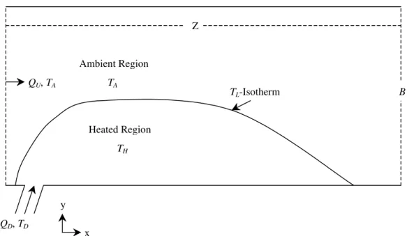
In the following sections of this paper, a set of equations is derived to model the dynamics of the thermal advection/diffusion processes that are caused by the discharge of stormwater effluent into a mixing zone of a water body. It is assumed that a fixed-volume mixing zone is allowed around the discharge point, where the water temperature can exceed the ambient temperature. The proposed model delineates the mixing zone into two regions, ambient and heated, based on water temperature (see Figure 1). Development of the model is guided by the assumption that the primary concern is with heat plumes that exceed a defined threshold temperature TL, which is greater than the ambient water temperature TA. Temperatures above
TL could harm the aquatic biota but for temperatures below TL no harmful effects should
occur. The ambient region is the part of the mixing zone where the water temperature is less than the threshold temperature (and above the ambient water temperature). For the model formulation, the water temperature of the ambient region is assumed to be constant and equal to TA. The heated region is where the water temperature exceeds the threshold temperature TL
and within this region the water temperature can vary with time. The size, duration, and temperature of the heated region are the focus of the model development.
The TL-isotherm in the mixing zone forms the boundary between the ambient and heated
regions (see Figure 1). The motion of the isotherm is governed by the amount of energy that is needed to raise the water temperature from TA to TL and this energy is determined by the net
heat flux at the boundary surface. This is similar to a Stefan condition (Crank, 1984) in heat conduction problems where the fusion/melting isotherm delineates the liquid and solid regions of a material that is undergoing a phase transition due to heating or cooling. However for the problem described herein, instead of a phase transition occurring at the boundary between the ambient and heated regions there is an instantaneous temperature jump from TA
to TL (see Figure 2). The Stefan condition is also extended to include the heat fluxes due to
advection at this boundary.
The model that is presented in this paper can be used to study the effects of time-varying discharge rates and temperatures, caused by different weather events (or series of events) and urban surface temperatures, on the size and temperature of the heated region in a water body. Results from such studies provide a means of focusing efforts on the key weather scenarios and urban surface temperatures that could adversely affect the aquatic ecosystem of a water body and that could require more detailed modelling and possible field studies to identify options for mitigating these effects.
MODEL PRELIMINARIES
Consider a region, as shown in Figure 1, which depicts a mixing zone for a stormwater discharge point that is located on the bottom shoreline. The average width of the mixing zone is B (in the transverse direction) and its length is Z (in the longitudinal direction). Let h be the depth of the zone throughout which the water is at thermal equilibrium, with no heat flux in the vertical direction. The value of h may represent the entire depth of the mixing zone or some fraction of it. For the time period under investigation, which will be hereafter referred to as the discharge transient, all dimensions of the mixing zone, and thus its volume, remain fixed. Prior to the start of the discharge transient, the ambient region, with water temperature
TA, occupies the entire mixing zone and the volumetric flow upstream of the discharge point is
x y Ambient Region Heated Region TL-Isotherm TA TH QU, TA QD, TD Z B
Figure 1. The mixing zone for the discharge of stormwater effluent into a receiving water body showing the division between the ambient and heated regions by the TL-isotherm.
The transient begins when stormwater effluent starts to enter the mixing zone. The
stormwater discharges into the mixing zone at a volumetric flow rate of QD and at a
temperature TD. Values for both parameters are expected to vary during the transient. The
cross sectional area of the discharge and its orientation relative to the mixing zone are known and fixed. The stormwater effluent mixes with the water body, transferring heat to it via turbulent diffusion and advection, and creates a heat plume that grows in the transverse and longitudinal directions downstream of the discharge point. The transient ceases when there is insufficient thermal power in the effluent (i.e., mass flow multiplied by stored thermal energy) to maintain the temperature in the plume above the threshold limit.
The mixing zone, with dimensions B, Z, and h, will define the fixed control volume VMZ for
this system. Two constituents can occupy VMZ: ambient water, which has a fixed temperature
TA, and heated water that can have a variable temperature TH ≥ TL. The ambient and heated
water occupy the sub-volumes VA and VH, respectively. These two sub-volumes can change
size with time but VMZ = VA + VH must always hold. Mass and energy can be exchanged
between the two sub-volumes and between VMZ and the environment (these processes will be
subsequently discussed). The stormwater runoff discharges into the heated region. A single, continuous TL-isotherm forms the interface between the two constituents. Motion of the TL
-isotherm is governed by the heat flux at the interface and is described in more detail in a later section.
The discharge transient is driven by the thermal power in the stormwater effluent, which is split between raising the temperature TH in the heated region and expanding its volume VH
through the conversion of ambient to heated water. The time rate of change of TH is modelled
by combining the mass and energy balances for the heated zone and the time rate of change of
VH is determined by modelling the movement of the TL-isotherm. With prescribed initial and
boundary conditions, the simultaneous solution of these two equations along with a momentum balance equation, to describe the velocity field in the mixing zone, can be used to simulate the discharge transient. Derivation of the local mass balance and the time rate of change of TH will be presented. Derivation of the momentum equation is left for future
research. First, attention is turned to deriving the differential equation for tracking the TL
-isotherm, which is the interface between the ambient and heated regions.
MOTION OF THE T
L-ISOTHERM
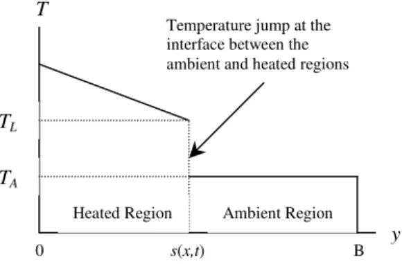
The motion of the interface between the ambient and heated regions will be treated using a Stefan condition (Crank, 1984) where the heat flux at the interface governs the conversion between ambient to heated water. Stefan conditions are typically applied to track the melting or fusion front in heat conduction problems. In such cases, the temperature profile is continuous across the interface between the material phases (as the temperature is held constant while latent energy is consumed or produced for the phase conversion). However, for this application a temperature discontinuity is assumed at the interface, as shown in Figure 2.
0 s(x,t) B
T
y TA
TL
Heated Region Ambient Region Temperature jump at the interface between the ambient and heated regions
Figure 2. Temperature profile between the ambient and heated regions.
Patel (1968) produced a general expression for the motion of the solidification (or melting) front for heat conduction problems. This expression will be used to describe the motion of the interface that separates the ambient and heated regions of the mixing zone. Let Ti be the
temperature along the interface of these two regions and be equal to the temperature limit TL,
i.e., Ti(x,s(x,t),t) = TL. Let TH and TA be the temperatures in the heated and ambient regions,
respectively, n be the outward normal vector at the interface (pointing into the ambient region), vn be the velocity of the interface in the normal direction, ρ be the average water
density in the two regions, ∆H be the energy required to increase the temperature of water from TA to TL, and qn be the net heat flux to the interface from other sources in the normal
direction. With these definitions, the energy balance at the interface can be expressed as:
(
)
L i x s x t t T T , ( , ), =( )
n n A A H H H v q n T k n T k = ∆ − ∂ ∂ − ∂ ∂ ρAs mentioned above, the expression that Patel formulated was for tracking the motion of a solidification (or melting) front. Thus in the above equation ∆H was defined as the latent heat produced or consumed to change material phases but not temperature, however, for the application in this paper ∆H is the amount of energy consumed to change a unit mass of water from the ambient “phase” to the heated “phase” and this produces a temperature change from
TA to TL in that mass of water. As there is no spatial temperature gradient in the ambient
region, i.e. the water in entire region is at temperature TA, the second term of the above
(
L A)
n n p H H c T T v q n T k = − − ∂ ∂ ρwhere cp is the specific heat of water. For the range of temperatures that would be considered
for this type of problem (e.g. 4°C to 40°C), the difference in cp is less than one percent (Haar,
1984; NBS/NRC, 2002) and is, therefore, assumed to be constant. This equation can be re-written to express the velocity of the interface as a balance of the heat fluxes:
(
)
⎟⎠ ⎞ ⎜ ⎝ ⎛ + ∂ ∂ − = H n H A L p n q n T k T T c v ρ 1For this two-dimensional problem, the transverse coordinate can be expressed as a function of the longitudinal coordinate, i.e., y=s(x,t), and the above equation can be reduced to one-dimension using relationships derived by Patel:
(
)
⎟⎟ ⎠ ⎞ ⎜ ⎜ ⎝ ⎛ + ∂ ∂ − ∂ ∂ ⎥ ⎥ ⎦ ⎤ ⎢ ⎢ ⎣ ⎡ + ⎟ ⎠ ⎞ ⎜ ⎝ ⎛ ∂ ∂ − = ∂ ∂ y x H H A L p q x s q y T k x s T T c t s 1 1 2 ρwhere qx and qy are x- and y-components of the advective heat flux, respectively. For heat
conduction applications, kH is the thermal diffusivity of the material, however, for the
application in this paper the thermal diffusivity will be expressed as a function of the turbulent
diffusion coefficient Dy. These relationships are as follows:
p y H D c k = ρ
(
L A p s x x u c T T q = , ρ −)
where ux,s =ux(
x,s(x,t),t)
(
L A p s y y u c T T q = , ρ −)
where uy,s =uy(
x,s(x,t),t)
Note that in the above expressions the parameters ux,s and uy,s are respectively the x- and
y-components of velocity at the interface. Substitution of these expressions into the above equation and simplification of the terms yields:
(
)
xs ys H y A L u x s u y T D x s T T t s , , 2 1 1 + ∂ ∂ − ∂ ∂ ⎥ ⎥ ⎦ ⎤ ⎢ ⎢ ⎣ ⎡ + ⎟ ⎠ ⎞ ⎜ ⎝ ⎛ ∂ ∂ − = ∂ ∂ (1)This expression relates the movement of the interface between the ambient and heated regions
at every point along the TL-isotherm to the heat fluxes caused by turbulent diffusion and
advection. The author believes this to be the first application of Patel’s interface conditions to an advection-diffusion problem. This equation coupled with the local mass balance and the time rate of change for the temperature in the heated region (which is discussed in the next section), and the appropriate initial and boundary conditions can be used to simulate the transient behaviour of a heat plume in a receiving water body that is caused by discharging stormwater effluent.
TEMPERATURE OF THE HEATED REGION
In the previous section, an equation was derived to model the movement of the TL-isotherm
within the mixing zone, which translates into modelling the volume expansion/contraction of the heated region. Solution of this equation requires the transverse temperature gradient
within the heated region at each location adjacent to the TL-isotherm. The approach taken
here is to derive a one-dimensional, differential equation for the time rate of change of TH at
each point along the longitudinal axis (x-axis) of the heated region and to define TH(x,t) to be
the transverse-averaged temperature at each point x. The transverse temperature gradient is then approximated with a polynomial function (which will be discussed later in this section).
The time rate of change for TH is modelled by combining the mass and energy balance
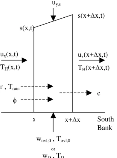
equations for the heated region. Figure 3 shows the mass and energy processes that act upon
a differential element of the heated zone. The differential element, ∆x, is selected to be small
enough that the curve s(x,t) is approximated by a straight line in the interval (x,x+∆x). In
Figure 3, the differential element is shown attached to the south bank of the water body, which is representative of a wall-attached heated region and is a common effluent configuration (Demetracopoulos and Stefan, 1983). The derivations of the balance equations that are presented herein will assume this type of geometry for the heated region. Derivations for heated regions that are partially detached will include elements that are bounded above and below by s(x,t) and will require equations of motion for the interface at both boundaries.
x+∆x x ux(x,t) TH(x,t) ux(x+∆x,t) TH(x+∆x,t) wovl,0 , Tovl,0 or wD , TD uy,s r , Train φ e s(x,t) s(x+∆x,t) South Bank
Figure 3. The mass and energy processes that act upon a fluid element in the heated region.
Mass and Energy Processes
Advection. Without loss of generality, flow entering the fluid element will be positive (for
both the x- and y-components) and negative for flow exiting the element. The flow velocity through the cross sectional area s(x,t)×h will be the average velocity over this cross section
and be denoted as ux(x,t). As mentioned above, the water temperature is averaged over the
length s(x,t) and is denoted by TH(x,t). Likewise the flow velocity and temperature exiting the
element through the cross sectional area s(x+∆x,t)×h is -ux(x+∆x,t) and TH(x+∆x,t),
respectively. The y-component velocity through the cross sectional area ∆x×h at the interface
is uy(x,t) and has a temperature of TL. For the mass and energy balances, the discharge flow
Lateral Flows. Flows from the banks of the water body into the heated region will be treated
as lateral flows and be defined per unit length along the longitudinal axis (with dimensions
m2/s). Lateral flows will be separated into two categories: discharge (wD) and overland flows
(wovl). The discharge flow is that resulting from stormwater effluent entering the heated
region and overland flow accounts for direct runoff from the bank into the heated region.
Rainfall. As the purpose of this model is to examine the effects of heat addition from
stormwater effluent on a water body, it is expected that some portion of the transient will include rainfall. Although rainfall may have a minimal effect on the mass balance in the heated region, it could influence its temperature and, therefore, it should be considered in the model. The rainfall parameter, r, is in depth per unit time (m/s).
Evaporation and Convection. Evaporative and convective losses will be treated as a single
process (i.e., with application of the Bowen Ratio) and will collectively be termed as evaporation. During the rainfall phase of the transient, evaporation may be minimal but for the post-rainfall phase where stormwater continues to discharge into the water body evaporation can occur. The evaporation parameter, e, is in depth per unit time (m/s).
Absorbed Solar Radiation. As with evaporation, during the rainfall phase of the transient the
effects of this process on the time rate of change of TH may be minimal but for the
post-rainfall phase of the transient it may be important. The solar radiation parameter, φ, is
expressed as a net heat flux with units of W/m2.
Mass Balance Equation
The time rate of change of mass per unit of longitudinal length (kg/(m⋅s)) in the heated region can be written as:
(
)
t t x s h u h w w e r s x u s h dt t x dM s y ovl dis x H ∂ ∂ + − + + − + ∂ ∂ − = ( , ) ) , ( , 0 , 0 , ρ ρ ρ ρ ρ ρ (2)where MH(x,t) is the mass of water in the volume h×dx×s(x,t) in the heated region at time t.
The first five terms on the R.H.S. of Equation 2 are the continuity terms for the element and
the last term accounts for the expansion/contraction due to the movement of the TL-isotherm
(see previous section). Assuming water to be incompressible over the temperatures and pressures for this type of problem, the sum of the continuity terms is equal to zero. Therefore, the change of mass for the heated region is only caused by expansion/contraction of its volume, i.e., the last term. However, the continuity terms are kept as they help simplify the
equation for the time rate of change of TH (as will be shown later). For the range of
temperatures that would be considered for this type of problem (e.g. 4°C to 40°C), the
difference in the density of water, ρ, is less than one percent (Haar, 1984; NBS/NRC, 2002)
and is, therefore, assumed to be constant.
Energy Balance Equation
The time rate of change in energy per unit of longitudinal length (W/m) in the heated region is:
( )
(
)
(
)
) , ( ) , ( ) , ( ) , ( , , 0 , 0 , t x s t t x s hT c u hT c w T c w T c e t x T r T s c x t x T u s h c t t x E L p s y L p ovl ovl p dis dis p H rain p H x p H ⋅ + ∂ ∂ + − + + − + ∂ ∂ − = ∂ ∂ φ ρ ρ ρ ρ ρ ρ (3)where cp is the specific heat of water and is assumed constant for the range of temperatures
considered in this problem type (see discussion in previous section), Train is the temperature of
the rainwater, TD is the temperature of the stormwater effluent at the discharge point, Tovl is
the temperature of the overland flow entering the mixing zone at location x on the south bank,
and φ is the net heat flux due to solar radiation.
Time Rate of Change for the Temperature of the Heated Region
This change in energy can also be expressed in terms of the volume expansion of the element and the change in water temperature in the element:
( )
(
( ) ( )
)
t t x T t x M c t t x M t x T c t t x T t x M c t t x E H H p H H p H H p H ∂ ∂ + ∂ ∂ = ∂ ∂ = ∂ ∂ ( , ) ) , ( ) , ( ) , ( , , ,By substituting Equation 2 and the above equation into Equation 3, the following expression is obtained (note that the (x,t) indices are omitted):
(
)
(
)
(
)
s t s hT c u hT c w T c w T c e T r T s c x T u s h c t T M c t s h u h w w e r s x u s h c T c L p s y L p ovl ovl p D D p H rain p H x p H H p s y ovl dis x p H p ⋅ + ∂ ∂ + − + + − + ∂ ∂ − = ∂ ∂ + ⎥⎦ ⎤ ⎢⎣ ⎡ ∂ ∂ + − + + − + ∂ ∂ − φ ρ ρ ρ ρ ρ ρ ρ ρ ρ ρ ρ ρ , 0 , , 0 ,Dividing through by ρcp and collecting terms, the above equation yields the time rate of
change for temperature in the heated region:
(
)
(
)
(
)
(
)
(
)
h c T T t s s T T s u T T hs w T T hs w T T h r x T u t T p H L H L s y H ovl ovl H D D H rain H x H ρ φ + − ∂ ∂ + − − − + − + − + ∂ ∂ − = ∂ ∂ 1 , 0 , 0 , (4)The above equation compactly describes the processes that affect the time rate of change of a fluid element in the heated region. Simultaneous solution of Equations 1, 2 and 4 yield solutions for ux, s(x,t), and TH(x,t) where the parameters r, Train, wD, TD, wovl,0, Tovl,0, and φ are
assumed to be known time-varying boundary conditions. Closure relations are needed for the velocities at the TL-isotherm (ux,s, and uy,s) and for the lateral temperature gradients (∂TH / ∂y).
The velocities ux,s and uy,s require either the solution of the momentum balance for the entire
mixing zone or some method to approximate them. This is the focus of future research efforts.
Approximation of the lateral temperature gradient
Solution of Equation 1, which describes the motion of the TL-isotherm, requires the lateral
temperature gradient (∂TH / ∂y) in the heated region at the interface (recall that there is no
gradient is to formulate the problem in two spatial dimensions and directly solve for TH(x,y,t)
and from the solution obtain the necessary gradients. The main drawback to this option is that a lot of computational overhead is created to obtain gradients that are only needed near the interface. Also, the calculated gradients could be sensitive to the mesh spacing. Another option is to approximate the temperature gradient with an assumed profile that can be matched to values already calculated. For example, a linear temperature profile can be simply
derived knowing that the temperature at the interface is TL and the average temperature of the
x-element is TH(x,t). The constant lateral gradient resulting from this profile is:
(
)
) , ( ) , ( 2 ) , ( t x s t x T T t x y TH L− H = ∂ ∂By adding the assumption that there is no lateral heat transfer at y=0 (i.e., between the water and the south bank of the water body in Figure 1), a quadratic temperature profile can be expressed in the form:
(
)
(
)
2 2 ( , ) ) , ( 2 3 ) , ( 3 2 1 ) , , ( T T x t y t x s T t x T t y x TH = H − L + L− HThe lateral gradient, at the interface, that results from this profile is:
(
)
) , ( ) , ( 3 ) , ( ) , ( s x t t x T T t x y T L H t x s y H = − ∂ ∂ =This gradient is larger than the one from the linear profile and will thus induce a faster volume expansion. Comparisons to experimental data and to two-dimensional numerical solutions will be needed to determine if either approximation is suitable for this application.
SUMMARY
A set of equations was derived to model the dynamics of the thermal advection/diffusion processes that are caused by the discharge of stormwater effluent into a mixing zone of a water body. The main features of this model are:
• Definition of a mixing zone that is divided into two regions, ambient and heated, which are separated by an isotherm that is the threshold temperature limit for the water body. By defining the mixing zone in this manner, one can model the duration, size, and temperature of the region that exceeds a temperature threshold given the time-varying conditions of the stormwater discharge into the water body.
• Formulation of an equation to describe the motion of the threshold temperature
isotherm (TL-isotherm). This equation permits one to model the size of the heated
region as a function of time. The motion of the isotherm is governed by the net heat flux at the boundary surface, which is similar to a Stefan condition in heat conduction problems but is extended to include the heat fluxes at the boundary due to advection. • An equation to describe the time rate of change of the water temperature in the heated
region. This equation allows one to model the magnitude that the temperature exceeds the threshold in the heated region, as a function of time.
Future research efforts will focus on the development of the momentum balance equation for
the mixing zone so that the velocities at the TL-isotherm (i.e., ux,s and uy,s) can be calculated.
Work will also proceed on a numerical solution method for the equations, which will likely draw upon previous work on the Isotherm Migration Method (Crank and Gupta, 1975; Crank, 1984).
ACKNOWLEDGEMENTS
The author would like to thank Drs. Yafei Hu and Maruf Mortula at the Centre for Sustainable Infrastructure Research, National Research Council of Canada, for their reviews and insightful comments.
REFERENCES
Crank, J. and Gupta, R.S. (1975), Isotherm migration method in two dimensions, International Journal of Heat and Mass Transfer, 18, pp 1101-1107.
Crank, J. (1984), Free and Moving Boundary Problems, Oxford University Press, Oxford, England.
Demetracopoulos, A.C. and Stefan, H. (1983), Transverse mixing in wide and shallow river: case study, Journal of Environmental Engineering, ASCE, 109, pp 685-699.
Harelman, D.R.F. and Stolzenbach K.D. (1972), Fluid mechanics of heat disposal from power generation, Annual Review of Fluid Mechanics, 4, pp 7-32.
Haar, L., Gallagher, J. and Kell, G. (1984), NBS/NRC Steam Tables: Thermodynamic and Transport Properties and Computer Programs for Vapor and Liquid States of Water in SI Units, Hemisphere Publishing Corporation, Washington, D.C.
James, W. and Xie, J.D.M. (1999), Storm water heating of urban streams, Proceedings of the Annual Conference of the Canadian Society of Civil Engineers, Regina, Saskatchewan, June 2-5, pp 569-578.
Jirka, G.H. (2007), Buoyant surface discharges into water bodies II: jet integral model, Journal of Hydraulic Engineering, 133(9), pp 1021-1036.
Jones, G.R. (1990), CORMIX3: An expert systems for the analysis and prediction of buoyant surface discharges, Masters Thesis, Cornell University, Ithaca, New York.
Kieser, M.S., Spoelstra, J.A., Fang, A.F., James, W. and Li, Y. (2004), Stormwater thermal enrichment in urban watersheds, Water Environment Research Foundation (WERF) Report 00-WSM-7UR, IWA Publishing, London.
Li, Y. and James, W. (2004), Thermal enrichment by urban stormwater: application to an urban area shopping mall and treatment wetland, Innovative Modeling of Urban Water Systems, Monograph 12, CHI Publishing, Guelph, Ontario, Canada, pp 665-682.
McGuirk, J.J. and Rodi, W. (1976), Calculation of three-dimensional surface jets, Proceedings of the 9th International Conference on Heat and Mass Transfer, Dubrovnik, Yugoslavia, pp 275-287.
NBS/NRC (2002), Steam Table Routines, http://orion.math.iastate.edu/burkardt/f_src/steam/steam.html, Last update on February 2, 2002.
Patel, P.D. (1968), Interface conditions in heat conduction problems with change of phase, AIAA J., 6, 2454. Stefan, H., Hayakawa, N., and Schiebe, F.R. (1971), Surface discharge on heated water, EPA-16130-FSU-12/71,
Minnesota University, Minneapolis, Minnesota.
Stefan, H. and Gulliver, J.S. (1978), Effluent mixing zone in a shallow river, Journal of the Environmental Engineering Division, ASCE, 104, 199-213.
Stefan, H. (1982), Mixing of the metro wastewater treatment plant effluent with the Mississippi River below St. Paul, Project Report No. 214, St. Anthony Falls Hydraulic Laboratory, University of Minnesota, Minneapolis, Minnesota.
Stolzenbach, K.D. and Harleman, D.R.F. (1971), An analytical and experimental investigation of surface discharges of heated water, EPA-16130-DJU-02/71, Ralph Parsons Laboratory for Water Resources and Hydrodynamics, Massachusetts Institute of Technology, Cambridge, Massachusetts.
Stolzenbach, K.D. and Harleman, D.R.F. (1973), Three-dimensional heated surface jets, Water Resources Research, 9(1), pp 129-137.
Van Buren, M.A.V. (1999), Thermal enrichment of urban receiving waters, Ph.D. Thesis, Queens University, Kingston, Ontario, Canada.
Verspagen, B. (1995), Experimental investigation of thermal enrichment of stormwater runoff from two paving surfaces, Masters Thesis, University of Guelph, Guelph, Ontario, Canada.