Active Pitch Control of an Oscillating Foil
with Biologically-Inspired Boundary Layer Feedback
by
Hemant Kumar Chaurasia
Bachelor of Science and Bachelor of Engineering (Honours) (2008)
Monash University (Australia)
Submitted to the Department of Aeronautics and Astronautics
in partial fulfillment of the requirements for the degree of
Master of Science
at the
MASSACHUSETTS INSTITUTE OF TECHNOLOGY
June 2010
c
° Massachusetts Institute of Technology 2010. All rights reserved.
Author . . . .
Department of Aeronautics and Astronautics
May 21, 2010
Certified by . . . .
Jaime Peraire
Professor of Aeronautics and Astronautics
Thesis Supervisor
Accepted by . . . .
Eytan H. Modiano
Associate Professor of Aeronautics and Astronautics
Chair, Committee on Graduate Students
Active Pitch Control of an Oscillating Foil
with Biologically-Inspired Boundary Layer Feedback
by
Hemant Kumar Chaurasia
Submitted to the Department of Aeronautics and Astronautics on May 21, 2010, in partial fulfillment of the
requirements for the degree of Master of Science
Abstract
We present a high-fidelity numerical study of a two-dimensional flapping airfoil, ad-dressing the hypothesis that boundary layer feedback control can enable improved performance in flapping flight. To this end, we model a novel biologically-inspired feedback controller which adjusts wing motion in response to the flow-induced bend-ing load experienced by sensory hairs mounted on the wbend-ing. Such hairs have been observed on bats, and biological studies suggest that an associated feedback controller may play an important role in enabling bats’ well-known mastery of flight.
The coupled fluid and structural equations of our model are solved numerically by a Discontinuous Galerkin finite element method, combined with an Arbitrary Lagrangian-Eulerian (ALE) formulation to account for airfoil motion. Feedback con-trol is defined by a simple proportional-derivative (PD) concon-trol law relating hair sensor feedback to an applied torque at the pivot point of the wing. We also include a tor-sional spring at the pivot point to model passive aeroelasticity, following prior work by Israeli [5].
Our results show that hair sensors are well-suited for detecting flow separation, and sensors placed near the leading edge enable better flight performance than sensors placed near the trailing edge. We compute a “performance envelope” for a purely passive flapping airfoil, and demonstrate that our active feedback controller enables improvements of up to 5% in propulsive efficiency. We also present gust alleviation experiments, where we find that an optimal PD controller reduces lift deviation by 33% compared to a spring-only airfoil. Mechanisms for these performance improvements are discussed. Our findings suggest that boundary layer feedback control may plausibly contribute to the outstanding flight abilities of bats, and may also provide valuable clues for designing robust and maneuverable Micro Air Vehicles (MAVs).
Thesis Supervisor: Jaime Peraire
Acknowledgments
This thesis would not have been possible without the invaluable guidance and support of my thesis advisor, Professor Jaime Peraire. My research has benefited in many ways from his patience, creativity, and the clear and insightful perspective he shares in our discussions. I am deeply grateful for his contributions to this thesis and to my devel-opment as a researcher. I would also like to acknowledge Professor Mark Drela for his help in framing my research problem, Dr. Cuong Nguyen for his encouragement, Pro-fessor David Darmofal and ProPro-fessor Youssef Marzouk for raising thought-provoking questions about my research, Professor David Willis for help with my flapping flight model, Dr. Benjamin Dickinson for sharing useful thoughts on hair sensor modeling, and Dr. Susanne Sterbing-D’Angelo for biological data on sensory hairs.
In many ways this thesis builds upon the earlier work of Emily Israeli, and I am greatly indebted to her for her generous support throughout this project. Thanks to Emily I not only had a great starting point for my work, but I also had someone I knew I could bug with questions anytime and get cheerfully useful answers – by any account, a rare privilege.
I would like to thank all of my labmates in the Aerospace Computational Design Lab for their contributions and camaraderie. In particular, I thank Pritesh Mody for many productive discussions about unsteady aerodynamics, for his friendship, and for keeping me sane on many occasions. I also thank Alejandra Uranga for keeping me on track when I needed it most; Isaac Asher for his help with the flapping flight code; Xun Huan and Eric Liu for cheerfully sharing the wild ride that is MIT; Thanh Huynh for his kindness as a colleague and friend; David Morol for his encouragement and that cup of tea the day before my quals; Masa, Huafei, Laslo and J.M. for making me believe that I could pass quals; Britt Rasmussen for bluffing in poker and threatening to beat me in getfit; David Lazzara for his contagious sense of calm; and Andrew March for sharing useful ideas about my results and how to survive a wedding. Beyond the lab, I would like to thank Matthew Fitzgerald for raising thought-provoking research
questions all the way from Melbourne, Australia; Kirstie Close and James Barry for projecting much care and encouragement from the same far-flung home; and Hiten Mulchandani, Sydney Do, Zach Bailey, Jon Allison, Russ Stratton, Georgia Smith and the aforementioned Mr. Mody for being good mates and sharing many fun times at MIT.
Importantly, I would like to thank my Mum, Dad and sister Ritu for cheering me on with such love and enthusiasm that even a silly thing like the Pacific Ocean could never get in the way. You are the weekly cure for MIT imposter syndrome, and if I had a nickel for every time you’ve made me smile or laugh, I would have a whole lot of nickels.
To my fianc´e Dilani: this thesis stands as yet another unreachable star that you have brought into my reach, and I know it will not be the last. You are a never-ending source of smiles, fun, confidence and stick-to-itiveness that make a world of difference every day. It is thanks to your encouragement and infectious disbelief in the impossible that I find myself submitting this Master’s thesis at MIT.
Finally, I wish to gratefully acknowledge the financial support for this work pro-vided by the US Air Force Office of Scientific Research through the MURI project on “Biologically-Inspired Flight for Micro Air Vehicles”.
Contents
1 Introduction 13
1.1 Motivation: Flapping Flight . . . 13
1.2 Objective and Approach . . . 15
1.3 Outline of Thesis . . . 16
2 Physical Model of Flapping Flight with Active Feedback Control 19 2.1 System and Assumptions . . . 19
2.2 Key Nondimensional Parameters of Flapping Flight . . . 21
2.3 Boundary Layer Hair Sensor Model . . . 23
2.4 Governing Equations of Motion . . . 26
3 Computational Approach 29 3.1 Numerical Evaluation of Hair Sensor Signal . . . 29
3.2 Discretization of Governing Equations . . . 32
3.3 Implementation and Execution . . . 35
4 Flapping Flight Results 37 4.1 Numerical Convergence Study . . . 37
4.2 Hair Sensor Signal Characterization . . . 42
4.3 Performance of Purely Passive System . . . 49
4.4 Performance of System with Proportional Feedback Controller . . . 50
5 Gust Alleviation Results 59 5.1 Experimental Procedure . . . 59
5.2 Optimal Control of Lift Deviation . . . 62
6 Conclusions 69
6.1 Summary of Findings . . . 69
6.2 Future Work . . . 71
A Notation and Sign Conventions 73
List of Figures
2-1 Physical model of oscillating foil with active feedback control . . . 20
2-2 Diagram of hair sensor model . . . 24
2-3 Illustration of feedback sensor signal definition . . . 25
3-1 Time-dependent mesh mapping used to implement airfoil motion . . . . 33
4-1 Grid resolution study for flapping flight simulations . . . 39
4-2 Computational mesh . . . 40
4-3 Close-up of computational mesh near airfoil surface . . . 40
4-4 Time resolution study for flapping flight simulations . . . 41
4-5 Transient analysis to determine appropriate length of time domain . . . 42
4-6 Visualization of flow solution for a typical spring-only flapping case . . 43
4-7 Typical timeseries of hair sensor feedback signal during flapping flight . 45 4-8 Correlation between hair bending moment and boundary layer shape factor at the same location. . . 45
4-9 Time-series of feedback signal X(t) at different sensor locations . . . . 47
4-10 Frequency spectrum of feedback signal X(t) at different sensor locations 48 4-11 Performance envelopes for purely passive and actively feedback-controlled flappers . . . 51
4-12 Effect of feedback controller on total torque applied to the airfoil . . . . 53
5-1 Initial condition for gust alleviation experiments . . . 61
5-3 Controller gain space showing optimal gust alleviation, with a spring . 64
5-4 Comparison of transient lift response with and without optimal control 65
5-5 Controller gain space showing optimal gust alleviation, without a spring 66
List of Tables
4.1 Propulsive efficiency as a function of sensor location . . . 46
5.1 Control gain parameters studied for gust alleviation experiment . . . . 62
A.1 Summary of Notation and Sign Conventions (Part I) . . . 73
Chapter 1
Introduction
1.1
Motivation: Flapping Flight
A growing interest in Micro Air Vehicles (MAVs) has motivated a renewed focus on understanding natural flapping flight. Natural flyers are capable of outstanding maneuverability and robustness in flight, characteristics which presently elude our best examples of artificial bird-sized flying devices. Flapping flyers such as birds and bats exploit a complex combination of unsteady aerodynamics, fluid-structure interaction and active control to achieve their outstanding mastery of flight. A deeper understanding of the physics behind Nature’s solution to small-scale flight is of great interest: intrinsically, biologically, and for the potential to yield insights that aid in the design of more capable MAVs.
In looking to understand natural flapping flight, a reasonable course of action would be to study the species with the most advanced mastery of flight. Bats are known to be particularly adept flyers – for example, the fruit bat species Cynopterus brachyotis is known to be capable of extreme maneuvers such as 180◦ turns at 200◦s−1 in a space
of less than half its wingspan [14]. Bat species such as Eptesicus fuscus are aerial predators, capturing winged prey in mid-flight [18]. Metabolic studies also suggest that bats fly 20-25% more efficiently than birds [16]. Bats are the only mammals to have evolved the ability of powered flight, and they have highly articulated wings with
a far more intricate 3D wing motion than birds or insects. Bats achieve their mastery of flight despite the complicated low Reynolds number, transitional flow regime in which they operate.
We seek to understand the special features of bat flight that may enable their unique agility in the air. One hypothesis put forward by biologists concerns small hairs seen distributed over the surface of bat wings [2]. These hairs are distinct in size and length from regular pelage hair; they grow out of dome-shaped complexes identified as touch-sensitive cells; and they are well-represented in the somatosensory cortex of the bat [12]. Further, recent work by Dickinson [3] finds that the observed lengths of these bat hairs are similar to the theoretical optimum for sensitivity to changes in the boundary layer. This collection of anatomical evidence suggests that bats may use these hairs as airflow sensors, providing real-time information about the boundary layer flow over their wings. It is hypothesized that these hair sensors are part of an active feedback control system by which the bat fine-tunes its wing motion in response to flow changes in the boundary layer, thereby improving flight performance and robustness.
Direct testing of this active feedback control hypothesis has so far been difficult to obtain. To the best of the author’s knowledge, there is only one relevant biological experiment reported in the literature: a very briefly described study by J. M. Zook [18]. In this experiment, two individual bats of the species Eptesicus fuscus were trained to fly a course involving a 90◦ turn, and the vertical elevation of each bat was
recorded over the length of the course. After 10 trials, sensory hairs were removed from the wings of both bats by means of a hair removal cream. The bats were then made to fly 10 more trials on the test course, again measuring flight elevation over the length of the course. In this manner, the experiment intended to directly measure the effect of sensory hairs on flight performance.
Analysis of the flight elevation data showed that an absence of sensory hairs was associated with a substantial drop in the bats’ flight elevation during the 90◦ turn. If
perfor-mance in bats. One plausible explanation is that the bats use their wing sensory hairs to help estimate lift during maneuvers, and they make adjustments to wing motion based on that estimation. This idea explains why an absence of sensory hairs might result in a loss of elevation through the 90◦ turn. It also supports the general
hypoth-esis that wing sensory hairs are used as part of an active feedback control system for wing motion.
The results of these biological experiments are tantalizing at best, leaving open an opportunity for a more rigorous examination of the hair sensor feedback control hypothesis for bat flight. If we can show that boundary layer feedback control enables substantial improvements in flight performance, this will lend further support to the hypothesis and provide new insights into Nature’s solution to small-scale flight. With artificial hair sensors currently under development [7], these insights may also prove relevant to the design of high-performance flapping MAVs in the near future.
1.2
Objective and Approach
The objective of this thesis is to characterize the performance of a biologically-inspired
active feedback controller for flapping flight. The particular form of this controller is
chosen to mimic the hypothesized boundary layer sensing function of hairs found on bat wings (see Section 1.1).
Our analysis seeks to address 3 key research questions:
1. What kinds of inputs work well for this type of active feedback controller?
2. How much can flight performance be improved by this type of active feedback controller?
3. What are the mechanisms for these improvements?
The present work addresses these questions through a high-fidelity numerical study of a pitching and heaving 2D airfoil, serving as a simplified model of flapping flight.
We solve the full Navier-Stokes equations using a Discontinuous Galerkin finite ele-ment method and account for time-varying geometry using an Arbitrary Lagrangian-Eulerian (ALE) formulation. The heaving motion of the airfoil is a prescribed sinu-soidal function of time, and its pitching motion is governed by a combination of passive aeroelasticity and active feedback control. The active feedback controller mimics the hypothesized boundary layer sensing function of hair sensors on bat wings.
This extends previous work by Israeli [5] on a similar physical model that featured passive aeroelasticity but lacked any element of boundary sensing or feedback control. In the present thesis we augment this purely passive model to include hair sensors and an associated feedback controller. With this new model we are able to characterize the flight performance of an actively feedback-controlled flapping airfoil and compare it against a purely passive one, highlighting the unique performance capabilities brought about by feedback control.
1.3
Outline of Thesis
The remainder of this thesis is organized as follows.
Chapter 2 presents a detailed introduction to our physical model of a flapping airfoil with biologically-inspired feedback control. Here we specify our hair sensor model, feedback controller, and several important properties of our 2D physical model. Key nondimensional parameters and figures of merit are also defined, namely the Strouhal number, reduced frequency, thrust coefficient and propulsive efficiency. This leads to a definition of the governing equations of motion for the overall physical model.
Chapter 3 presents an outline of the computational approach used to numerically solve the governing equations, including the Discontinuous Galerkin finite element method and the Arbitrary Lagrangian-Eulerian formulation employed to account for time-varying geometry. Discretization of the governing equations in both space and time is addressed. The numerical implementation of our hair sensor feedback and active controller is specified in some detail, including mention of the 3DG code which
our computational tool is built upon.
Chapters 4 and 5 present the results of our physical investigations, conducted using the computational tools described above. In Chapter 4 we present results pertaining to cruising flapping flight, including a characterization of the hair sensor signal and the effect of hair sensor location on flight performance. Grid and time resolution studies are presented that justify our choice of computational mesh, timestep size and time domain length. We then present a performance envelope of a purely passive flapping airfoil in terms of thrust and propulsive efficiency, and compare this envelope to that attainable with the addition of our hair sensor feedback controller. The mech-anisms behind the observed improvements are discussed. Chapter 5 presents results pertaining to gust alleviation, analyzing the ability of our active feedback controller to suppress the lift transient associated with an Euler vortex passing over an airfoil that was previously in a steady flow at fixed angle of attack. We find that the active feedback controller is able to suppress this lift transient more effectively than pas-sive aeroelasticity alone, and we offer insights into what mechanisms may drive this improvement.
Finally, Chapter 6 provides a summary of our findings and suggests directions for future work. For quick reference, Appendix A contains a summary of all notation and sign conventions used in this thesis.
Chapter 2
Physical Model of Flapping Flight
with Active Feedback Control
This chapter presents a detailed introduction to our physical model of a flapping airfoil with biologically-inspired feedback control. Here we specify our hair sensor model, feedback controller, and several important properties of our 2D physical model. Key nondimensional parameters and figures of merit are also defined, leading to a definition of the governing equations of motion for the overall physical system.
2.1
System and Assumptions
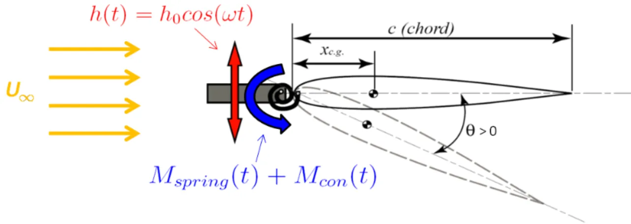
Figure 2-1 illustrates the physical model studied in the present work. We consider a two-dimensional symmetric airfoil hinged at the leading edge, undergoing a prescribed vertical heaving oscillation combined with a pitching motion about its leading edge. The airfoil is in a uniform horizontal freestream of velocity U∞, or equivalently, the
airfoil is traveling through still air with a forward speed U∞. The airfoil’s pitching
motion is governed by a combination of moment imparted by the fluid, inertia of the airfoil, passive aeroelasticity and active feedback control. Passive aeroelasticity is modeled through a single torsional spring located at the leading edge. The airfoil itself is rigid but exhibits aeroelastic pitching behavior via the leading edge torsional
Figure 2-1: Physical model of oscillating foil with active feedback control.
spring. This spring applies a pitch-dependent restoring torque Ms = Csθ, where Cs
is the spring stiffness and θ is the airfoil pitch angle. The active feedback controller applies an additional control torque Mc at the leading edge, where Mc is a function of
the feedback signal returned by hair sensors on the wing.
Our simulations are conducted at a chord Reynolds number of Re = 5, 000 and are fully laminar. While this Reynolds number is somewhat lower than the Re ∼ 40, 000 of natural bat flight, it allows us to avoid the difficult complications associated with modeling unsteady turbulent transition, whilst still capturing a large part of the physics. It should also be noted that the Re = 5, 000 regime has unambiguous relevance to biological (and artificial) flapping flyers the size of large insects.
Other flow properties in our model include the Mach number (where we choose Ma = 0.2), the Prandtl number (where we choose Pr = 0.72), and the ratio of specific heats (where we choose γ = 1.4). The latter two values are standard choices for atmospheric air at sea level, and the Mach number is simply chosen low enough to make any compressibility effects negligible. A more physically precise value of the Mach number for bat flight would be on the order of Ma ∼ 0.02, however we do not expect any substantial differences if we were to repeat our simulations with Mach number 0.02 instead of 0.2. Choosing Mach number 0.2 also allows direct comparisons between the present work and that by Israeli [5], which used Mach number 0.2.
6.5%. This is similar to the thickness ratios observed on natural airfoils across a range of bird species including the swift, petrel and woodcock [17]. The moment of inertia of the airfoil about its pivot point is chosen to be I = 0.033, a choice which allows the airfoil’s rotational inertia to be neither negligible nor dominant. A more comprehensive study of the effect of different I values on flapping flight performance is left for future work.
In our study, the vertical heaving motion is an input parameter h(t). We choose a sinusoidal motion h(t) = h0cos(ωt), where h0 is the heaving amplitude and ω is
the heaving frequency. The pitching motion of the airfoil is effectively a complicated response to this input. By varying h0and ω we may obtain different levels of thrust and
propulsive efficiency. Several other system parameters also affect thrust and propulsive efficiency, such as the spring stiffness Cs and the precise definition of the feedback
control law.
2.2
Key Nondimensional Parameters of Flapping
Flight
We now define key nondimensional parameters of flapping flight, as are relevant to the present study. The heaving motion of the wing is described by a nondimensional amplitude and frequency, which are the Strouhal number St and the reduced frequency
k respectively. These are defined:
St = ωh0/πU∞ (2.1)
k = ωc/2U∞ (2.2)
Here, U∞is the uniform steady freestream velocity and c is the chord length of the
airfoil. h0 and ω are the dimensional heaving amplitude and frequency. In Nature, all
in the range 0.2 to 0.4 [13]. Accordingly, the present study focuses on a narrow range of Strouhal numbers centered on St = 0.2 to 0.4. Also drawing inspiration from Nature, we choose a reduced frequency of k = 0.4. This is close to the reduced frequency observed in the medium sized bat species Cynopterus brachyotis flying at low to medium speeds [4]. A study of other values of k is left for future work, in order to avoid an impracticably large parameter space in the present thesis.
Aside from these key input parameters, we define two key figures of merit to measure performance of a particular flapping motion. These figures of merit are the nondimensional thrust coefficient CT and the propulsive efficiency ηprop, defined below.
CT = −1 T RT 0 D(t) dt 1 2ρU∞2c (2.3) ηprop = Pout Pin (2.4) Here T is the heaving oscillation period and ρ is the fluid density. D(t) is the
x-component of the total aerodynamic force on the airfoil, where a negative D(t)
represents positive thrust. Pin is the average power input to drive the airfoil motion,
and Pout is the average power output in terms of thrust. These are defined as below:
Pin = 1 T Z T 0 ³ −L(t) ˙h(t) − Mc(t) ˙θ(t) ´ dt (2.5) Pout = 1 T Z T 0 −D(t)U∞ dt (2.6)
Here L(t) is the y-component of the total aerodynamic force on the airfoil, and thus −L(t) ˙h(t) is the rate of work that must be done to heave the airfoil vertically according to the heaving function h(t). Mc(t) is the torque applied at the leading edge
of the airfoil by the feedback controller, and thus Mc(t) ˙θ(t) is the rate of work done
by the feedback controller to actuate the pitching motion of the airfoil. Note that the passive aeroelastic torque Csθ(t) also drives the pitching motion of the airfoil, but
since it is driven by a perfectly elastic spring, the net amount of work done by the spring is zero and it does not appear in the expression for Pin.
2.3
Boundary Layer Hair Sensor Model
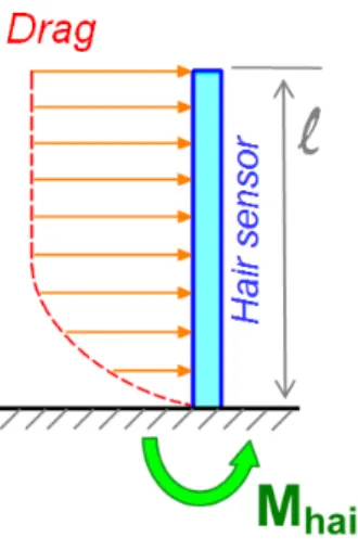
We now describe our model boundary layer feedback sensor, intended to mimic the hypothesized function of sensory hairs on bat wings. Sensory hairs on bat wings grow out of dome-shaped complexes containing high concentrations of touch-sensitive Merkel cells. These cells respond when they are stretched or strained, and our hair sensor hypothesis contends that this response is primarily triggered by mechanical load induced by deflection of the hair in airflow.
We adopt a simplified model of this process, consisting of a straight cylindrical hair of contant cross-section mounted perpendicular to the surface of the wing. This model was first employed by Dickinson [3], who successfully argued that the flow over such sensory hairs is inertia-free and quasi-steady – that is, the hair is effectively motionless on the timescales of the fluid flow. It was also noted that the tip deflection of such a hair in an extreme case would be no more than 10% of the hair length. In our model we make a further simplification and simply neglect any deflection of the hair. As the actual deflection would be quite small, the no-deflection approximation should not have any appreciable quantitative effect on our numerical experiment.
In our hair sensor model, touch-sensitive cells are activated by the bending moment felt at the base of the hair due to aerodynamic load over the length of the hair. This is illustrated in Figure 2-2. The aerodynamic load on the hair at each lengthwise location is taken to be the drag force that would be experienced by an infinite circular cylinder of the same diameter in a uniform incident flowfield, where the velocity of the hypothetical uniform flowfield matches the flow velocity measured at that particular point along the hair. Note that in our model, we neglect any effect on the flowfield due to the presence of the hair. We may write down the bending moment at the base of the hair, Mh, as:
Figure 2-2: Diagram of hair sensor model, showing equilibrium of torques about the base of the hair.
Mh(t) = Z l 0 1 2CD(Rey)ρu 2d 0y dy (2.7)
Here we use the empirical drag coefficient CD(Rey) for a circular cylinder in a
crossflow, where Rey = ρd0u(y)/µ is the local Reynolds number at a position y along
the length l of the hair. The hair has a diameter d0. The density and velocity of
the bulk fluid at the position y are ρ and u respectively, and the velocity u includes only the component perpendicular to the hair. This approximation for the drag on the hair relies upon a quasi-steady assumption, as justified by Dickinson [3]. Note also that, in keeping with data presented by Dickinson [3], we choose the hair length
l such that it is taller than the boundary layer thickness by a reasonable margin
(mimicking the observed lengths of bat hairs). For the cases we have studied, we found
l = 0.2 to be a sufficient length to guarantee this (by visual inspection of boundary
layer velocity profiles for a range of extreme cases). Also note that we define the sensory hair diameter as d0/c = 10−4, which is the same order of magnitude as typical
measurements of bat hairs [3]. This diameter also ensures the local Reynolds number is well within the Stokes flow regime.
Spatial distribution of hair sensors is another important parameter of our sensor model. In bats, hair sensors are observed to be distributed over the entire surface of
Figure 2-3: Diagram illustrating the definition of our feedback sensor signal: the difference between the bending moments at the base of two hairs above and below the wing at the same chordwise location.
the wing [12, 18]. It seems likely that a bat’s flow sensing process combines information from all of these hairs in a complicated manner. Rather than attempting to replicate this system in all its detail, in our model we employ only two hair sensors located above and below the wing at the same chordwise position (Figure 2-3). This serves as the simplest possible example of a distributed hair sensor network. Denoting the feedback sensor signal as X(t), we choose to take the difference between the hair bending moment Mh at these two hairs above and below the wing:
X(t) = Mh(A, t) − Mh(B, t) (2.8)
As we will describe in the next section, our feedback control law is defined such that the active control torque applied at the leading edge of the airfoil is a function of X(t). The particular form of X(t) described in Equation 2.8 guarantees that for a symmetric wing motion, freestream and airfoil, the signal X(t) will be symmetric and have zero mean, and thus so too will the torque applied by the controller. In the present study we choose to only explore flapping wing motions which preserve symmetry in this manner; hence our definition in Equation 2.8. However, we note that there is another class of signal definitions X and feedback control laws that generally lack this symmetry and lead to asymmetric forces and wing motions. For
example, an asymmetric airfoil would very likely lead to this kind of behavior. An investigation of such sensing and control configurations is beyond the scope of the present thesis, but is mentioned here as an interesting topic for future work.
2.4
Governing Equations of Motion
Here we present the key governing equations of our physical model. First we define the form of our active feedback control law. In keeping with the theme of simplicity in the present work, we choose to study a proportional-derivative (PD) control law with feedback signal X (Equation 2.8) and control actuation torque Mc:
Mc(t) = KpX(t) + KdX(t)˙ (2.9)
Here, Kp and Kd are constant proportional and derivative gains respectively. This
PD control law constitutes a very simple approximation of the internal processes that a bat may employ to process feedback from its hair sensors and decide upon a corrective action. The form of this control law is not in any way biologically inspired – rather, it is chosen as the simplest possible functional relationship between a feedback sensor signal X(t) and a corrective action Mc(t). Our goal is to assess whether even in this
simplest of cases, an active feedback control law can lead to an improvement in flight performance.
With this active control torque defined, we can now define a 2nd-order structural
equation of motion for the airfoil, which can be expressed as two 1st-order equations
as follows:
˙θ − w = 0 (2.10)
I ˙w(t) + Csθ(t) + Mc(t) + Mf luid(t) − S¨h(t) = 0 (2.11)
pitching rate of the airfoil, Cs is the torsional spring stiffness, Mf luid is the moment
imparted by the fluid about the pivot point of the airfoil, S is the static mass imbalance of the airfoil and ¨h(t) is the acceleration of the pivot point in the vertical direction. Each of the five terms in Equation 2.11 in turn represent: the rotational inertia of the airfoil, passive aeroelasticity, active feedback control, fluid-structure interaction, and the torque derived from the airfoil’s static mass imbalance.
Note that in Equation 2.11, the Mc term is a function of X which is in turn a
function of the flowfield. Mf luid is also a function of the flowfield. Thus, these two
terms encode the fluid-structure interaction behavior of the flapping airfoil.
To describe the fluid flowfield itself we employ the full Navier-Stokes equations, which can be written in the conservative form:
∂u
∂t + ∇ · Fi(u) − ∇ · Fv(u, ∇u) = 0 (2.12)
with inviscid fluxes Fi, viscous fluxes Fv and fluid state vector u. (The particular
form of these fluxes and state vector may be found in many sources, for example in [5].)
Note that in our simulations we will be directly measuring boundary layer quan-tities and driving the motion of the airfoil according to these measurements, via the feedback control law (Equation 2.9). Thus, the accuracy of our simulations will de-pend strongly upon how well they represent the unsteady boundary layer over the wing, and this is why we must solve no less than the full Navier-Stokes equations.
Chapter 3
Computational Approach
This chapter presents an outline of the computational approach used to numerically solve the governing equations of our physical model, including the Discontinuous Galerkin finite element method and the Arbitrary Lagrangian-Eulerian formulation employed to account for time-varying geometry. Discretization of the governing equa-tions in both space and time is addressed. The numerical implementation of our hair sensor feedback and active controller is specified in some detail, including mention of the 3DG code which our computational tool is built upon.
3.1
Numerical Evaluation of Hair Sensor Signal
A key element of our numerical solver is an algorithm for computing hair bending moments Mh and hence the feedback sensor signal X (Equations 2.7 & 2.8), given a
flowfield u and structural state (θ, w). As described in Section 2.3, our model hair sensors respond to the flowfield but not vice-versa. It is assumed that the presence of a hair sensor does not alter the flowfield in any way. Thus, the task of calculating the bending moment Mh at the base of a given hair simply amounts to evaluating an
integral of flow quantities over a predetermined line. In particular, the line represents the location, size and orientation of the hair sensor. Since our model hair sensors are assumed straight and unable to deflect or deform, this predetermined line will be fixed
and unchanged in relation to the airfoil for each individual hair sensor.
In our model, hair sensors are located with their base on the surface of the airfoil and they extend perpendicularly outward from the airfoil. Using the known airfoil profile coordinates, it is simple to determine the equation of a line corresponding to a given hair. To evaluate the Mh line integral defined by Equation 2.7, we apply the
trapezoidal method to a set of integrand values evaluated at discrete points along the line. The length of each hair is l = 0.2, and we choose to take 120 sample points along each hair for the numerical quadrature. This number of sample points is chosen because it is high enough to render any quadrature error insignificant.
This gives us a set of points (xi, yi) at which to evaluate the integrand of
Equa-tion 2.7, and in order to proceed we must interpolate the flow soluEqua-tion at each of these points. To perform the interpolation, we first note the structure of the spatial discretization employed by the Discontinuous Galerkin finite element method. The spatial domain is discretized into a computational mesh of many triangular elements, and on each element there are ns nodal points. The overall numerical solution is
repre-sented as an elementwise polynomial function, and within each element the numerical solution is expressed in terms of a nodal basis of polynomial shape functions φ. Each of the ns nodal points has an associated shape function φj. Using these shape
func-tions, a solution quantity such as vertical flow velocity v may be interpolated at any point within an element as follows:
v(ξi, ηi) = ns
X
j=1
vjφj(ξi, ηi) (3.1)
where φj(ξi, ηi) is the polynomial shape function associated with the jth nodal
point, vj are the values of v known at each of the nodal points, and (ξi, ηi) are the
reference coordinates of the point at which we wish to interpolate v. These reference coordinates (ξi, ηi) are distinct from the global coordinates (xi, yi) in that they take
values between 0 and 1 and are only defined on a single element, whereas the global coordinates (xi, yi) are defined throughout the computational domain.
Thus, given a set of points (xi, yi) at which we wish to evaluate interpolated flow
quantities, our task becomes one of converting global coordinates into element numbers and reference coordinates. That is, for each sample point (xi, yi), we must identify
the particular element containing that point and the associated reference coordinates (ξi, ηi). We can then apply the method shown in Equation 3.1 to correctly interpolate
any desired flow quantity at the chosen sample point.
To convert these global coordinates (xi, yi) into an element number and reference
coordinates (ξi, ηi), we take a two-step approach. First, we identify the nearest mesh
vertex to the sample point and list all the elements that share that vertex. The nearest neighbors of those elements are also listed. This forms a set of candidate elements that the point (xi, yi) may reside in. On each of the candidate elements, we then attempt
to find the reference coordinates (ξ, η) which drive the following two residuals to zero:
Rx(ξ, η) = xi− ns X j=1 xjφj(ξ, η) (3.2) Ry(ξ, η) = yi− ns X j=1 yjφj(ξ, η) (3.3)
Note that the right-hand side of these residual equations simply expresses the difference between the sample point (xi, yi) and the interpolated global coordinates at
(ξ, η). In our code implementation, we drive the residuals Rx and Ry to zero using
a Newton-Raphson method with an under-relaxation factor of 0.6, necessary to avoid bad behavior when the initial guess for (ξ, η) is far from the correct value. If a pair (ξ, η) is found that sets both residuals to zero, and the (ξ, η) values also satisfy the requirement that they are between 0 and 1, then we have found the correct element and reference coordinates corresponding to the given sample point (xi, yi). If the reference
coordinates that set Rx and Ry to zero are not within the range 0 to 1, then we can
infer that the sample point does not reside in that particular element, and we move on to try another candidate element in the list until the correct element and reference coordinates are found.
In this manner, all the sample points (xi, yi) along a given hair may be converted
into element numbers and associated reference coordinates (ξi, ηi). Since the hairs do
not move relative to the airfoil and we choose a non-deforming computational mesh, these element numbers and reference coordinates need only be solved once rather than at every timestep. With these values in hand, flow quantities may be easily interpolated as shown in Equation 3.1; numerical quadrature may be performed to yield Mh (Equation 2.7); and the Mh values may be combined to give the feedback
signal X(t) (Equation 2.8). This is how the hair sensor feedback signal X is evaluated within our numerical model at each timestep.
3.2
Discretization of Governing Equations
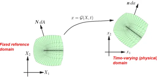
To solve the governing equations of our physical model (Section 2.4) we employ a high order Discontinuous Galerkin finite element spatial discretization, using Roe’s scheme for inviscid fluxes [11] and the Compact Discontinuous Galerkin (CDG) formulation for the viscous fluxes [9]. To account for the time-dependent geometry associated with the motion of the airfoil, we employ an Arbitrary Lagrangian-Eulerian (ALE) formulation of the kind presented by Persson, Bonet & Peraire [10]. In our implementation, the entire mesh is rigidly translated and rotated according to the time-dependent motion of the airfoil (see Figure 3-1). A time-dependent mapping G(X, t) relates a stationary reference domain to the time-dependent physical domain. This mapping is used to define a form of the fluid equations (Equation 2.12) that may be solved on the fixed reference domain. The reference domain solution can then be mapped to the time-varying domain to provide the true physical flowfield. A detailed derivation of this mapping is presented by Israeli [5] and Persson, Bonet & Peraire [10].
To couple the fluid equations (Equation 2.12) and the structural equations (Equa-tions 2.10 & 2.11), we first recast them as systems of 1st-order equations. We then
append the structural discretized equations to the fluid discretized equations and ap-pend the structural degrees of freedom to the fluid degrees of freedom, thus obtaining
Figure 3-1: Diagram illustrating the time-dependent mesh mapping used to implement airfoil motion in our simulations.
a system in terms of an overall state vector U. This results in a system of ordinary differential equations with a mass matrix M and nonlinear residual vector R(U):
MdU
dt = −R(U) (3.4)
These equations are integrated forward in time using a 2nd-order accurate backward
Euler implicit scheme, also known as a backward difference formula (BDF; or BDF2 for 2nd order). This time-stepping scheme approximates the time derivative as a weighted sum of the state vector U at the new time-level n and the two preceding time-levels:
∂U ∂t ' 1 ∆t 2 X i=0 ciUn−i (3.5)
where ci = (3/2, −2, 1/2) are the weighting constants for BDF2.
This expression yields an implicit system of equations for the new state vector
Un, which can be solved using a Newton-Raphson method with a Jacobian matrix
J = ∂R/∂U. At each iteration j of the Newton-Raphson method, we solve for a state
vector update ∆Un(j):
where the BDF residual and Jacobian matrix are defined with constants αi and βk: RBDF(Un(j)) = M 2 X i=0 αiUn−i− βk∆tR(Un) (3.7) J(Un(j)) = dRBDF dUn = α0M − βk∆t dR(Un) dUn ≡ M − βk∆tK (3.8)
For BDF2, the constants αiand βkare defined as αi = (1, −4/3, 1/3) and βk= 2/3
(they take different values for BDF orders different to 2).
For completeness, we also present here the form of the last two entries of the vector
R(Un(j)), which are residuals corresponding to the structural degrees of freedom θ and
w. These terms are derived from the structural equations of motion (Equations 2.10 &
2.11), and they encode all the fluid-structure interaction and active feedback control behavior of our physical model. The two residuals are:
Rθ(Un(j)) = wn (3.9) Rw(Un(j)) = − Cs I θ (j) n − K0 I X (j) n − Mf luid,n(j) I − Kd I∆t k X i=1 αkiXn−i+ S ¨hn I (3.10)
Here the subscript n denotes that the quantity is evaluated at the nth timestep,
and we also define:
K0 = Kp+
Kdα0
∆t (3.11)
The terms on the right-hand side of Equation 3.10 represent all the same effects that are contained in the original equation of motion (Equation 2.11) – that is, passive aeroelastic torque, active feedback control torque (expressed as a function of the sensor signal X), fluid-structure interaction and static mass imbalance. Note that the
deriva-tive portion of the feedback control torque in Equation 2.9 contains a time derivaderiva-tive of the feedback signal, ˙X. This time derivative is discretized in the residual equation
above using the same BDF2 formula (Equation 3.5) that was used to discretize the overall system of equations, simply for the sake of consistency.
With these residual equations in hand for both the structural degrees of freedom and the fluid degrees of freedom, we can take partial derivatives to define all entries of the Jacobian matrix J and set up a Newton-Raphson solver for our system of equations (Equation 3.4). With this solver in place, we can time-march from any initial condition and compute the behavior of a feedback-controlled flapping airfoil.
Note that in the formulation described above, a modest improvement in compu-tational efficiency could likely be gained by choosing a 2-stage Diagonally Implicit Runge-Kutta (DIRK) time-stepping scheme instead of BDF2. The use of a DIRK scheme also removes any start-up problems associated with initializing or restarting a time integration. Future work beyond this thesis will implement DIRK instead of BDF2, however for the results in the present thesis our numerical solutions are all based upon BDF2.
3.3
Implementation and Execution
Our implementation of this solver is built upon an in-house code called 3DG, which implements the Discontinuous Galerkin spatial discretization for a fluid-only system. This code is written in a combination of Matlab and C, and has been employed in prior published research including work by Nguyen et al [8] and Willis et al [15]. Work by Persson, Bonet & Peraire [10] and Israeli [5] extended this code to incorporate an ALE formulation and aeroelastic fluid-structure interaction respectively. For the present work, this code was further extended to incorporate our hair sensor feedback model and proportional-derivative feedback controller.
Simulations are run on a multi-processor desktop machine with 16 nodes, allowing up to 16 different cases to be run in parallel. An average flapping flight simulation
integrated over 7 heaving periods takes approximately 16 hours to complete, and this is representative of all cases that were run to generate the results presented in this thesis.
Chapter 4
Flapping Flight Results
Using the physical model and numerical simulation methodology described in the preceding chapters, studies were performed to investigate several physical aspects of feedback-controlled flapping flight. These included a characterization of the hair sen-sor signal, the performance envelope of a “purely passive” (spring-only) flapper, and the performance envelope of our actively feedback-controlled flapper. This chapter presents key results from these studies, including a numerical convergence study quan-tifying the convergence errors associated with our choice of spatial and time domain discretization.
4.1
Numerical Convergence Study
Beyond the computational methodology described in Chapter 3, it is necessary to choose a specific computational mesh, timestep size and time domain length for our simulations. These must be chosen carefully to ensure that our simulation results are not corrupted by numerical convergence errors of any appreciable size.
To guide our choices, a numerical convergence study was conducted on a single, par-ticularly demanding test case with high Strouhal number and large controller gains Kp
and Kd. Specifically, the test case had parameters St = 0.3, Kp = 2, 500, Kd = 3, 000
2.1. This single test case was run with a large range of different meshes, timestep sizes and time domain lengths, and the thrust coefficient CT and propulsive efficiency ηprop
were measured from each solution (CT and ηprop being our most important figures of
merit). Taking the finest discretization and longest time domain length as the “truth” value, we were thus able to calculate the numerical convergence error in CT and ηprop
due to each particular choice of discretization. Using this error as a metric, we could justify a particular choice of mesh, timestep and time domain length with which to perform all subsequent simulations, ensuring that numerical convergence errors remain within acceptable limits.
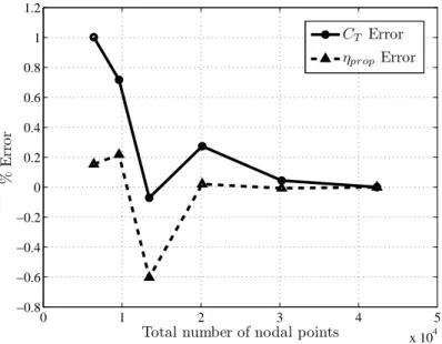
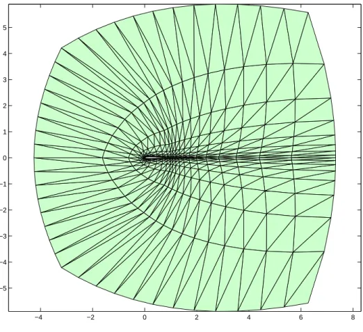
First was the grid resolution study. We chose to rely upon C-meshes rather than the unstructured meshes employed in [5]. From our study we found that solution quantities are quite sensitive to how well the airfoil’s wake is resolved, and C-meshes proved to be particularly efficient at providing grid resolution in the wake. We generated a series of C-meshes each with different numbers of elements and different polynomial degrees. One way to distinguish these meshes is by their total number of nodal points. After running the test case described above on all these meshes, including an extremely fine one to serve as the “truth” value, we obtained grid convergence results that are presented in Figure 4-1.
These results clearly show both CT and ηprop converging as mesh resolution is
increased, and importantly, the total numerical convergence error is never more than
∼1% even for the coarsest mesh studied. This is certainly within acceptable limits
for the purposes of our physical investigation. Ideally we would like to solve on the coarsest mesh possible, as it allows us to run more simulations in less time. Thus, we use Figure 4-1 to justify choosing the left-most mesh on that plot, a C-mesh with 640 elements and 3rd-order polynomials (totalling 6,400 nodal points). It has a domain
size of approximately 4 chord lengths in every direction from the airfoil, plus an extra chord length in the downstream direction. This mesh is plotted in Figure 4-2. It will be our standard mesh choice for all subsequent simulations in this thesis, as our grid resolution study indicates numerical convergence errors should mostly be within 1%.
0 1 2 3 4 5 x 10⁴ −0.8 −0.6 −0.4 −0.2 0 0.2 0.4 0.6 0.8 1 1.2
Total number of nodal points
% E rr o r CT Error ηpropError
Figure 4-1: Grid resolution study measuring error in averaged solution properties CT and ηprop as a function of different choices of mesh (denoted by their total number of nodal points). Error is measured as a percentage deviation from the CT and ηprop values obtained on the finest mesh (right-most point on the plot).
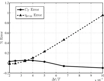
The next aspect of the discretization to specify was the timestep size. A time res-olution study was performed in much the same manner as the grid resres-olution study, repeating the same test case described above with many different timestep sizes over long-duration simulations (8 heaving periods each, with the CT and ηprop values
com-puted over the 8th period). The results of this study are presented in Figure 4-4
below, and they indicate that any of the timestep sizes presented here will satisfy a 1% tolerance on convergence error. Being more conservative with timestepping (since the feedback controller may introduce odd high-frequency behavior that we wish to capture), we select ∆t/T = 1/250 as our timestep size, bringing the convergence error estimate within ∼0.1%.
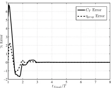
Finally, we must select an appropriate time domain length for our simulations. The beginning of a flapping flight simulation always includes some transient behavior that dies away over time as the solution approaches a truly periodic state. To quantify how long we must integrate in time to neglect transient effects, we conducted a transient analysis on our test case using the standard mesh choice and twice the time resolution.
−4 −2 0 2 4 6 8 −5 −4 −3 −2 −1 0 1 2 3 4 5
Figure 4-2: Plot of the computational mesh chosen as a result of our grid resolution study. The total convergence error associated with this mesh was within 1%. It has 640 elements and 3rd-order polynomials, for a total of 6,400 nodal points.
−0.2 0 0.2 0.4 0.6 0.8 1 −0.6 −0.4 −0.2 0 0.2 0.4
2 3 4 5 6 7 8 9 10 x 10−3 −0.2 0 0.2 0.4 0.6 0.8 1 1.2 ∆t/T % E rr o r CT Error ηpropError
Figure 4-4: Time resolution study measuring error in averaged solution properties CT and ηprop as a function of timestep size. Error is measured as a percentage deviation from the CT and ηprop values obtained by the smallest timestep size, ∆t/T = 5 × 10⁻⁴, which is 4 times smaller than the left-most datapoint on this plot.
We integrated forward in time over 8 heaving periods, and then computed the period-averaged quantities CT and ηprop over 1-period windows ending at a range of different
times tf inal. The results of this analysis are presented in Figure 4-5 below, and they
indicate that any time domain longer than approximately 4 heaving periods will be long enough to give at least 1 complete period of data where transient effects are essentially zero. Adding a conservative margin to this figure, we choose to select a standard time domain length of 7 heaving periods, computing CT and ηprop over
the final 2 periods of the time record. This effectively guarantees that numerical convergence error due to transient effects will be negligible (below 0.01%).
Thus we have justified a choice of mesh, timestep size and time domain length with expected convergence errors of approximately 1%, 0.1% and < 0.01% respectively. All subsequent simulations in this chapter have been run with this discretization, and from the figures above, we do not expect numerical convergence errors any larger than approximately 1% in total.
1 2 3 4 5 6 7 8 −2 −1 0 1 2 3 4 5 6 7 tf inal/T % E rr o r CT Error ηprop Error
Figure 4-5: Transient analysis showing how the period-averaged quantities CT and
ηprop converge as a function of which period they are averaged over. tf inal refers to the endpoint of the averaging period. Error is measured as a percentage deviation from the CT and ηprop values obtained from the 8th period. These results indicate that transient effects become negligible approximately 3 heaving periods after initialization.
4.2
Hair Sensor Signal Characterization
The first task in seeking physical understanding of our feedback-controlled flapping wing system was to characterize the hair sensor signal for a typical flapping cycle. To address this, we conducted simulations of a “purely passive” flapper where only the spring was allowed to apply torque to the leading edge of the airfoil. (That is, an instance of our physical model where Kp = Kd = 0.) During these simulations we
measured the feedback signal X(t) and analyzed its behavior. Note that here we only
measure the feedback signal – the control law gains are kept at Kp = Kd = 0 and we
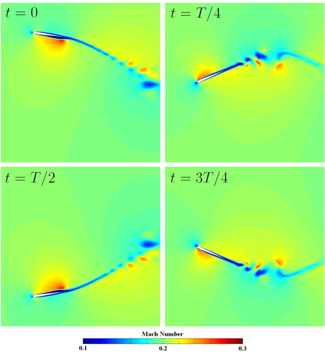
do not use the feedback signal to drive any control torque actuation. For purposes of illustration, Figure 4-6 presents a visualization of the flow solution for a typical example of a purely passive flapping case as described above.
Considering these purely passive cases with Kp = Kd = 0, Figure 4-7 presents a
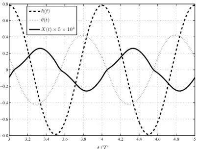
typical example of the measured feedback signal X(t) and its correlation with the wing pitch angle θ(t) and the leading edge vertical translation h(t). Observe that taking
Figure 4-6: Visualization of flow solution for a typical spring-only flapping case, with
Cs= 0.2, St = 0.2, k = 0.4, Kp = Kd= 0. The color contours measure Mach number, which is closely indicative of flow velocity in this low Mach number regime.
the difference between hair sensors above and below the wing results in a signal that is symmetric and has zero mean (as intended). But this alone doesn’t tell us very much about how an actively controlled system would behave with this feedback signal and nonzero controller gains.
What we would like to understand is the relationship between the hair sensor feedback signal and important physical properties of the flow over the wing. Flow separation over the wing has substantial consequences for the thrust and efficiency generated by the wing, and the boundary layer shape factor H is a good quantifier for the onset of flow separation. Figure 4-8 presents the measured correlation between the bending moment Mh at the base of a single hair sensor (note: Mh, not X) and the
boundary layer shape factor H computed at the location of that same hair. This yields an important observation: the output quantity of our hair sensors is well suited to sensing flow separation (H > 4). When the flow separates (H ≈ 4), the hair bending moment becomes high, and when the flow is far from separation, the hair bending moment is low. This correlation is evidence that our model hair sensors provide useful information about the flow. In particular, it suggests that it should be possible to design a feedback controller that selectively responds to conditions where the flow is getting close to separation. By encoding selective responses to the onset of flow separation, the feedback controller may help to avoid energetically lossy wing motions and thereby improve propulsive efficiency.
Another important aspect of our hair sensor feedback system is the spatial distri-bution of hair sensors. For simplicity, we have limited ourselves to a single pair of hair sensors located above and below the wing at a given chordwise location along the wing. This leaves us to choose a desired chordwise location, and we wish to choose the location that gives our feedback controller the best possible chance of improving propulsive efficiency.
To inform this decision, we performed a series of active control experiments with the same flapping and control parameters (i.e. St, Cs, k, Kp, Kd) but different hair sensor
3 3.2 3.4 3.6 3.8 4 4.2 4.4 4.6 4.8 5 −0.8 −0.6 −0.4 −0.2 0 0.2 0.4 0.6 0.8 t/T h(t) θ(t) X (t) × 5 × 10⁴
Figure 4-7: Timeseries of wing leading edge vertical translation h(t), wing pitch angle
θ(t) radians, and the feedback signal X(t) acquired by differencing the hair bending
moment above and below the wing at a chordwise position x/c = 0.3. This data corresponds to a purely passive test case with spring stiffness Cs = 0.2, Strouhal number St = 0.2, and reduced frequency k = 0.4.
3 3.5 4 4.5 x 10⁻⁵ 2 2.5 3 3.5 4 4.5 Mh(t) H ( t)
Figure 4-8: Correlation between hair bending moment Mh (for a single hair) and boundary layer shape factor H at the same location. The hair in this case is located on the upper surface of the wing at x/c = 0.3 and has length L/c = 0.2. This data pertains to a flapping test case with spring stiffness Cs = 0.2, Strouhal number St = 0.2, reduced frequency k = 0.4 and no controller (Kp = Kd= 0).
Kd = 0. Hair sensors located near the front of the wing (x/c = 0.21) were compared
with hair sensors located further back (x/c = 0.3 and x/c = 0.7). The results of these experiments showed that the hair sensors nearest the leading edge produced wing motions with the highest propulsive efficiency, very similar to the x/c = 0.3 sensors but substantially higher than the x/c = 0.7 sensors (see Table 4.1 for one example). Not only was the propulsive efficiency higher, but the pitching motion of the airfoil was also inherently smoother than the violently chaotic motions observed with sensors at
x/c = 0.7. From these results we conclude that, for our model of hair sensor feedback
control, sensors placed nearer to the leading edge result in better flight performance than sensors placed nearer to the trailing edge. Specifically, leading edge hair sensors appear to enable higher propulsive efficiency. Accordingly, we choose to place our sensors near to the leading edge (x/c = 0.21) for all subsequent simulations in this thesis.
Table 4.1: Propulsive efficiency as a function of sensor location, for active control test cases with Kp = 104, Kd= 0, Cs = 0.2, St = 0.3 and k = 0.4
Sensor Location Propulsive Efficiency
x/c = 0.21 67.83%
x/c = 0.30 67.62%
x/c = 0.70 61.33%
While it is difficult to provide a rigorous and general theoretical explanation for this result, we can offer some insights that may partially explain what we have seen here. Our insights are based on measurements from a purely passive flapping test case identical to what was used in Figures 4-7 & 4-8. (Recall that by “purely passive” we mean that the feedback sensor signal is measured but not allowed to drive any control torque – that is, Kp = Kd = 0.) In one of these purely passive test cases,
the feedback sensor signal was measured at several different sensor locations, and the resulting timeseries are plotted in Figure 4-9.
3 3.2 3.4 3.6 3.8 4 4.2 4.4 4.6 4.8 5 −8 −6 −4 −2 0 2 4 6 8x 10 −6 t/T X (t ) x/c = 0.21 x/c = 0.3 x/c = 0.5 x/c = 0.7
Figure 4-9: Time-series of feedback signal X(t) at different sensor locations x/c, for a spring-only case with St = 0.2, Cs = 0.2, k = 0.4.
a feedback signal that is weaker, more lagged and less harmonic. This point is fur-ther clarified by Figure 4-10, which presents a single-sided amplitude spectrum of the timeseries data presented in Figure 4-9. These spectra indicate that higher harmonics are almost wholly absent in the feedback signal from the hair sensors at x/c = 0.21, but those higher harmonics are much more prevalent in the signals from sensors closer to the trailing edge. This may be due to shedding of vortical structures from the boundary layer, which disrupt the hair sensor feedback signal when they pass through the hair, and have a greater effect when the sensors are further downstream of the shedding point.
From our observations, we can surmise that these higher harmonics are an unde-sirable trait of a feedback signal in our proportional-only feedback controller (Kp > 0,
Kd= 0). Consider the fact that in our proportional feedback controller, the feedback
signal is scaled linearly to determine what control torque is applied at the leading edge. Higher harmonics in the feedback signal thus imply higher harmonics in the forcing applied at the wing leading edge. If these higher harmonics are large enough in
am-0 1 2 3 4 5 6 7 8 9 10 0 0.5 1 0 1 2 3 4 5 6 7 8 9 10 0 0.5 1 0 1 2 3 4 5 6 7 8 9 10 0 0.5 1 0 1 2 3 4 5 6 7 8 9 10 0 0.5 1 0 1 2 3 4 5 6 7 8 9 10 0 0.5 1
Frequency (in units of ω)
x/c = 0.21
x/c = 0.3
x/c = 0.5
x/c = 0.7
x/c = 0.9
Figure 4-10: Single-sided amplitude spectrum of feedback signal X(t) at different sen-sor locations x/c, for a spring-only case with St = 0.2, Cs = 0.2, k = 0.4. Frequency component amplitudes are normalized by the 1stharmonic. Note the increasing
preva-lence of higher harmonics in the feedback signal as we consider hair sensors located closer to the trailing edge of the wing.
plitude and frequency, they will have the effect of “jerking” the wing back and forth on a timescale much shorter than the heaving period, possibly promoting a greater degree of flow separation and vortex shedding that could further enhance high fre-quency wing motions. This could explain the relatively chaotic wing motion observed in test cases with sensors placed at x/c = 0.7. Also, an increase in flow separation and vortex shedding could explain the decrease in propulsive efficiency, since these are energetically lossy phenomena.
For now, a more complete explanation must remain a topic of further study. How-ever, on the empirical level we have fairly unambiguous evidence to support a signifi-cant conclusion: that our feedback-controlled flapping flight model performs at higher propulsive efficiency when the hair sensors are placed nearer to the leading edge.
4.3
Performance of Purely Passive System
We shift now towards seeking to understand the performance of a feedback-controlled flapping airfoil on a more global level. In order to assess the performance increment achieved by adding a feedback controller to our otherwise “purely passive” spring-only system, we first require a quantification of the overall performance capabilities of a purely passive flapping wing. Our two key figures of merit are thrust coefficient CT
and propulsive efficiency ηprop. To keep our comparison relatively simple, we limit
ourselves to a fixed reduced frequency of k = 0.4 and vary only Strouhal number St and the spring stiffness Cs.
If we perform a design sweep over a large range of (St, Cs) values, we may compute
thrust CT and efficiency ηprop as functions of the (St, Cs) parameter space. This study
has been performed by Israeli [5], and we use data presented there to define our own Pareto front in (CT, ηprop)-space for a purely passive system. That is, we take the
data from a large number of test cases with different (St, Cs) values, compute the
corresponding (CT, ηprop), and generate a scatterplot of the (CT, ηprop) values of all
our test cases. The convex hull of these points in (CT, ηprop)-space defines a Pareto
front that can be interpreted as a “performance envelope” for a purely passive system – that is, the maximum attainable propulsive efficiency as a function of total thrust.
It turns out that this Pareto front is very well approximated by the set of test cases which have spring stiffness Cs = 0.2. This echoes the findings of Israeli [5]
which indicated that Cs = 0.2 is an optimal spring stiffness with respect to propulsive
efficiency, over a broad range of thrust levels. Therefore, to simplify our treatment of the parameter space, we define the performance envelope of a purely passive system to be the maximum attainable propulsive efficiency with a spring stiffness of Cs= 0.2
and unconstrained Strouhal number. The resulting performance envelope is presented in Figure 4-11 as the thick green line. The test cases along this line differ only in Strouhal number, increasing monotonically from left to right on the plot (all other parameters are constant, including k = 0.4 and Cs = 0.2). This is the performance
baseline against which we will compare an actively feedback-controlled flapping airfoil.
4.4
Performance of System with Proportional
Feed-back Controller
The thick green line in Figure 4-11 defines the performance envelope of a purely passive flapper, and this shall be the baseline for our assessment of the performance incre-ment attainable by augincre-menting such a flapper with our biologically-inspired feedback controller. For the sake of simplicity, we will constrain ourselves to a proportional feedback controller and set Kd = 0 always. This adds one degree of freedom beyond
that which a purely passive system possesses, and our task is to quantify how far this will allow the performance envelope to extend in the direction of higher propulsive efficiency.
The method we employ is to take a set of test cases located along the passive performance envelope in (CT, ηprop)-space, replace the zero values of Kp with nonzero
values, and repeat the simulations. The constraints Cs= 0.2 and k = 0.4 are retained,
and the hair sensors remain always in the location x/c = 0.21. By systematically increasing Kp in the positive or negative directions from a given passive “base case”,
we generate a set of trajectories through (CT, ηprop)-space. Over a large number of such
trajectories, we gather enough feedback-controlled test cases to define a convex hull and hence a Pareto front, in much the same manner as the passive Pareto front was defined earlier. A portion of the Pareto front thus derived is presented as the upper thin blue line in Figure 4-11, and we can interpret this as the performance envelope for a flapping wing that possesses both passive aeroelasticity and our biologically-inspired feedback controller.
We immediately note an important observation: the performance envelope for the actively feedback-controlled system exceeds that of the purely passive system. The difference between these two curves is a literal expression of the performance improvement attainable by taking a spring-only flapper and augmenting it with a
hair-0 0.05 0.1 0.15 0.2 0.25 0.3 0.35 0.4 0 10 20 30 40 50 60 70 80 90 100 CT ηp r o p (% )
Spring-Only Performance Envelope
Spring and Proportional Controller Performance Envelope Spring and Proportional Controller Test Cases
Figure 4-11: Pareto fronts in the (thrust, efficiency) parameter space, for a spring-only system (thick green) and the same system augmented by our biologically-inspired pro-portional feedback controller (thin blue). These Pareto fronts can be interpreted as “performance envelopes” for the two systems, delineating the maximum propulsive ef-ficiency attainable at each given thrust level. Note that the feedback controlled system achieves propulsive efficiencies up to 5% higher than the spring-only performance enve-lope. The spring-only performance envelope is defined for reduced frequency k = 0.4, hair sensor location x/c = 0.21 and Strouhal number range St ∈ [0.1, 0.5]. It is also constrained to spring stiffness Cs = 0.2, a value demonstrated by Israeli [5] to yield optimal propulsive efficiency over a broad range of thrust levels (including those shown above). The spring+controller performance envelope is defined with the same restric-tions on k, x/c, St and Csand additionally allows the feedback controller proportional gain Kp to vary between 0 and 25, 000. The resulting set of Test Cases (marked with stars) are used to define a portion of the global performance envelope for the feedback controlled system, as shown above. Note that test cases with negative Kp are not shown, as they do not improve upon the spring-only performance envelope.