HAL Id: lirmm-03002261
https://hal-lirmm.ccsd.cnrs.fr/lirmm-03002261
Submitted on 12 Nov 2020
HAL is a multi-disciplinary open access
archive for the deposit and dissemination of
sci-entific research documents, whether they are
pub-lished or not. The documents may come from
teaching and research institutions in France or
abroad, or from public or private research centers.
L’archive ouverte pluridisciplinaire HAL, est
destinée au dépôt et à la diffusion de documents
scientifiques de niveau recherche, publiés ou non,
émanant des établissements d’enseignement et de
recherche français ou étrangers, des laboratoires
publics ou privés.
species identification with deep learning algorithms
Sébastien Villon, David Mouillot, Marc Chaumont, Gérard Subsol, Thomas
Claverie, Sébastien Villéger
To cite this version:
Sébastien Villon, David Mouillot, Marc Chaumont, Gérard Subsol, Thomas Claverie, et al.. A new
method to control error rates in automated species identification with deep learning algorithms.
Scien-tific Reports, Nature Publishing Group, 2020, 10 (1), �10.1038/s41598-020-67573-7�. �lirmm-03002261�
A new method to control error
rates in automated species
identification with deep learning
algorithms
Sébastien Villon
1,2*, David Mouillot
1,5, Marc Chaumont
2,3, Gérard Subsol
2,
Thomas Claverie
1,4& Sébastien Villéger
1Processing data from surveys using photos or videos remains a major bottleneck in ecology. Deep Learning Algorithms (DLAs) have been increasingly used to automatically identify organisms on images. However, despite recent advances, it remains difficult to control the error rate of such methods. Here, we proposed a new framework to control the error rate of DLAs. More precisely, for each species, a confidence threshold was automatically computed using a training dataset independent from the one used to train the DLAs. These species-specific thresholds were then used to post-process the outputs of the DLAs, assigning classification scores to each class for a given image including a new class called “unsure”. We applied this framework to a study case identifying 20 fish species from 13,232 underwater images on coral reefs. The overall rate of species misclassification decreased from 22% with the raw DLAs to 2.98% after post-processing using the thresholds defined to minimize the risk of misclassification. This new framework has the potential to unclog the bottleneck of information extraction from massive digital data while ensuring a high level of accuracy in biodiversity assessment.
In the context of accelerating human impacts on ecosystems1, the capacity to monitor biodiversity at large scale
and high frequency is an urgent although challenging goal2. This urgency resonates with the ambition of
inter-national initiatives like the Group on Earth Observations Biodiversity Observation Network (GEO BON) and the call for monitoring Essential Biodiversity Variables (EBVs)3,4.
Remote sensors are rapidly transforming biodiversity monitoring in its widest sense from individuals5 to
species and communities of species6. In the last decade, satellites7,8, drones9, 10, camera traps6, or underwater
cameras11,12 have been extensively deployed to record pictures or videos of aquatic and terrestrial organisms.
For instance, satellite data can be used to track whale shark movements13 or detect whales14 while photos from
airborne or underwater vehicles can deliver accurate density estimations of vulnerable organisms like mammals or sharks15,16.
Such massive records are also used by citizen science programs with for example public tools like inaturalist. org which share pictures and associated metadata, or fishpix (https ://fishp ix.kahak u.go.jp) which offers the pos-sibility to upload individual fish images that are then identified by experts at the species level.
However, processing photos or videos to identify organisms is a highly demanding task, especially in under-water environments, where some particular contexts add many difficulties (e.g., visual noise due to particles and small objects, complex 3D environment, color changing according to depth, etc.). For instance, identifying all fish individuals on videos may take up to 3 h of expert analysis per hour of video17. Under the avalanche of new
videos and images to analyse, alternatives to fish identification by humans and trained experts must be found. Recently, an effort to use machine learning methods18,19 and deep learning algorithms (DLAs) for
ecologi-cal analysis have been made, thanks especially to computer-vision challenges on public databases of annotated
open
1MARBEC, Univ of Montpellier, CNRS, IRD, Ifremer, Montpellier, France. 2Research-Team ICAR, LIRMM, Univ
of Montpellier, CNRS, Montpellier, France. 3University of Nîmes, Nîmes, France. 4CUFR Mayotte, Dembeni,
France. 5Australian Research Council Centre of Excellence for Coral Reef Studies, James Cook University,
photos or videos (e.g. for fish, Fish4Knowledge database (https ://group s.inf.ed.ac.uk/f4k/) and Seaclef challenge (https ://www.image clef.org/lifec lef/2017/sea)).
The last generation of DLAs offer much promise for passing the bottleneck of image or video analysis through automated species identification20–23. DLAs, and particularly convolutional neural networks (CNNs),
simultane-ously combine the automatic definition of image descriptors and the optimization of a classifier based on these descriptors24. Even though DLAs usually have a high accuracy rate, they do not provide information on the
confidence of the outputs. Hence, it remains difficult to identify and control potential misclassifications which limits their application.
Misclassification of images has two types of consequences for biodiversity monitoring. On one hand, if all individuals of a given species occurring in a given community are erroneously labelled as another species also occurring in the community, this species will be incorrectly listed as absent (false absence). The risk of missing present species because of misclassification is the highest for rare species, i.e. those with the lowest abundance in terms of the number of individuals per unit area. Yet missing these rare species can be critical for ecosystem heath assessment since some play important and unique roles like large parrotfishes on coral reefs25 while
oth-ers are invasive like the lionfish in Eastern Mediterranean Sea26. In addition, since most species in a community
are represented by a few individuals27, such misclassifications could significantly lead to the underestimation
of species richness. The other error associated with misclassification is when an individual of a given species is mistaken for another species not present in the community (false presence). Such misclassifications could lead to an overestimation of the abundance or geographical range of a species as well as it could artificially increase species richness, unless a species is consistently mistaken for another. Since biodiversity monitoring should be as accurate as possible, automated identification of individuals on images should provide high correct classification rates (close to 100%) even if a subset of images has not been classified by the algorithm with sufficient confidence and must be identified by humans a posteriori.
Chow28 was the first to introduce the concept of risk for a classification algorithm. For instance, a clustering
algorithm classifying an object placed in the center of a given cluster would present a low risk of misclassification, while classifying an object placed on the edge of a cluster would be highly risky. Chow28 proposed a classification
framework, which contains n + 1 channels as outputs, n channels for the n classes considered and an additional channel called the “rejection” channel. When the risk of misclassification is too important, the algorithm rejects the classification.
Applied to machine learning, a first method consists in learning a rejection function during the training, in parallel to the classification learning29–31. Another method, called a meta-algorithm, uses two algorithms, one
being a classifier, and the other one analyzing the classifier outputs, to distinguish predictions with a high risk of misclassification from those with a low risk32. A recent comparative study suggests that meta-algorithm-based
methods are the most efficient33.
An extension of meta-algorithms to control the risk of misclassification is to calibrate models obtained through Machine Learning and Deep Learning algorithms. Machine Learning methods usually produce well-calibrated models for binary tasks34. The calibration consists of a matching between the score predicted by the
machine-learning model and the real probability of true positives. While Deep Learning models produce more accurate classifications than other Machine learning models, these models are not well calibrated, and thus need a re-calibration to be used for real-world decisions35. Several propositions have been made to improve the
cali-bration of Machine Learning models through the post-processing of outputs. The Platt scaling36, the Histogram
binning37, the Isotonic Regression38 and the Bayesian Binning into Quantiles39 are mapping the model outputs
to real accuracy probabilities. More recently, Temperature Scaling, an extension of the Platt Scaling, was used to calibrate Deep Learning models using a single parameter for all classes35. This parameter is used, instead of
the traditional softmax function, to convert the vector output from the neural network into a real probability. However, such calibration methods are based on a discretization of the Deep model outputs into bins. Many bins are not useful as they only contain a few outputs with low values, whereas many high values fall in the same bin and are thus not discriminated. Moreover, the choice of the number of bins is left to the user, and therefore is not optimized to the Deep model nor to a specific application40.
In this paper, we present a simple, yet efficient method that accounts for uncertainty in the classifier outputs. Unlike calibration methods, our approach is not changing algorithm outputs. Instead, we simply assess the behav-iour of the model thanks to a validation dataset. We can then set-up a fine tuned threshold per class, allowing us to take into account that the model confidence can be highly variable between “easy” classes and “difficult” classes. Then, through the addition of a new class “unsure”, corresponding to predictions with scores lower than the predicted class threshold, we can control the coverage (total amount of images automatically identified) and misclassification rates. We applied this framework to classify 20 species of coral reef fishes in underwater images and assessed its efficiency for 3 real-case scenarios.
Material and methods
Data.
We decided to build our own dataset instead of using existing datasets (e.g. Fish4Knowledge: https :// group s.inf.ed.ac.uk/f4k/), to be in phase with quality of videos currently used by marine ecologists. We used 3 independent fish images datasets from the Mayotte Island (Western Indian Ocean) to train and test our CNN model and our post processing method. For the 3 datasets, we used fish images extracted from 175 underwa-ter high-definition videos which lasted between 5 and 21 min for a total of 83 h. The videos were recorded in 1920 × 1,080 pixels with GoPro Hero 3 + black and Hero 4 + black. The videos were recorded between 2 and 30 m deep, with a broad range of luminosity, transparency, and benthic environment conditions on fringing and bar-rier reefs.We extracted 5 frames per second from these videos. Then, we cropped images to include only one fish indi-vidual with its associated habitat in the background. Thus, images of the same species differed in terms of size (number of pixels), colors, body orientation, and background (e.g. other fish, reef, blue background) (Fig. 1).
We used 130 videos for the training dataset, from which we extracted a total 69,169 images of 20 different fish species (Supplementary Fig. S1). We extracted between 1,134 and 7,345 images per species.
In order to improve our model, we used data augmentation41 on native biodiversity and ecosystem. Each
“natural” image yielded 4 more images: 2 with increased contrast (120% and 140%) and 2 with decreased contrast (80% and 60%) (Supplementary Fig. S2). We then horizontally flipped all images to obtain our final training dataset (T0) composed of 691,690 images (Supplementary Table S1).
We then used two independent datasets made of different videos recorded on different days and on different sites than videos used to build the training dataset. The first dataset (T1) contained 6,320 images from 20 videos with at least 41 images per species, and the second (T2) contained 13,232 images from 25 videos with at least 55 images per species (Supplementary Table S1). We then used dataset T1 to tune the thresholds and T2 as the test dataset. This method ensures that our results are not biased by similar acquisition conditions between the training, tuning and testing dataset and hence that algorithm performance was evaluated using a realistic full cross-validation procedure.
Building the convolutional neural network.
Convolutional neural networks (CNNs) belong to the class of DLAs. For the case of species identification, the training phase is supervised, which means that the classes to identify are pre-defined by human experts while the parameters of the classifier are automatically optimized in order to accurately classify a “training” database24. CNNs are composed of neurons, which areorganized in layers. Each neuron of a layer computes an operation on the input data and transfers the extracted information to the neurons of the next layer. The specificity of CNNs is to build a descriptor for the input image data and the classifier at the same time, ensuring they are both optimized for each other42. The neurons
extract-ing the characteristics from the input data in order to build the descriptors are called convolutional neurons, as they apply convolutions, i.e. they modify the value of one pixel according to a linear weighted combination of the values of the neighbor pixels. In our case, each image used to train the CNN is coded as 3 matrices with numeric values describing the color component (R, G, B) of the pixel. The optimization of the parameters of the CNN is achieved during the training through a process called back-propagation. Back-propagation consists of automati-cally changing parameters of the CNN through the comparison between its output and the correct class of the training element to eventually improve the final classifications rate. Here we used a 100-layer CNN based on the TensorFlow43 implementation of ResNet44. The ResNet architecture achieved the best results on ImageNet Large Figure 1. Diversity of individual images and their environment for the same fish species (Moorish idol, Zanclus
Scale Visual Recognition Competition (ILSVRC) in 2015, considered as the most challenging image classifica-tion competiclassifica-tion. It is still one of the best classificaclassifica-tion algorithms, while being very easy to use and implement. All fish images extracted from the videos to build our datasets were resized to 64 × 64 pixels before being processed by the CNN. Our training procedure lasted 600,000 iterations; each iteration processed a batch of 16 images, which means that the 691,690 images of the training dataset were analyzed 14 times each by the network on average. We then stopped the training to prevent from overfitting45, as an over fit model is too restrictive and
only able to classify images that were used during the training.
Assigning a confidence score to the CNN outputs.
The last layer of our architecture, as in most CNNs, is a “softmax” layer44. When input data passing through the network reaches this layer, a function is applied toconvert the image descriptors into a list of n scores Si , with i = {1, .., n}, and n the number of learned classes (here
the 20 different fish species), with the sum of all scores equal to 1. A high score means a “higher chance” for a given image to belong to the predicted class. However, a CNN often outputs a class with a very high score (more than 0.9) even in case of misclassification. To prevent misclassifications, the classifier should thus be able to add a risk or a confidence criterion to its outputs.
Assessing the risk of misclassification by the CNN.
For a given input image, a CNN returns a pre-dicted class, in our case a fish species. As seen in the previous section, the CNN outputs a decision based on the score, without any information on the risk of making an error (i.e. a misclassification). Following De Stefano et al.32, we thus propose to apply a post-processing step on the CNN outputs in order to accept or reject itsclas-sification decision. The hypothesis is that the higher the similarity between an unknown image and the images used for the training, the stronger the activation in the CNN during the classification process (i.e. the higher the score is), and thus, the more robust the classification is.
For this method, the learning protocol is thus made of two consecutive steps performed on 2 independent training datasets.
• In the first phase, a classification model is built by training a CNN on a given database T0 (Fig. 2a)
• Then, the second phase consists of tuning a risk threshold τi specific to each class (i.e. each species in our
case), noted i, with i ∈ {1, ..., n} , using a second and independent database noted T1 (Fig. 2b).
In terms of classification, it means we transform the 2 classification options (correct, wrong) in 3 options (Fig. 3) by applying Eqs. (15, 16).
Computing the confidence thresholds.
After the phase 1 (model training phase), for an image X of the threshold tuning dataset processed by the classifier, we obtain an output {C(X), S(X)} , where C(X) is the class (i.e. species, belonging to the trained set of species) with the highest classification score S(X). For this image, we know the ground truth Y in {1, .., n} belonging to the same set of species classes.So with C(X) being the output class, Y the ground truth class, and #(.) the enumeration function, the standard definition for Correctly Classified images (or true positives) rate of a class i is:
We can also write the standard definition of Misclassified images rate (or false negatives) of a class i as:
Then, we can extend the Correct Classification rate (CC) and Misclassification (MC) rate of a species i by introducing the thresholds τi and by adding the Unsure Classification (UC) rate:
For each species we have:
We can also note that the standard coverage definition (COV, the rate of images for which a classification is given) of a species i can be extend with the introduction of thresholds as threshold τ as:
(1) CCi=#(C(X) = i AND Y = i) #Y = i (2) MCi= #(C(X) �= i AND Y = i) #Y = i (3) CCi(τi) = #((C(X) = i)AND(S(X) > τi))AND(Y = i) #(Y = i) (4) MCi(τi) = #((C(X) �= i)AND(S(X) > τi))AND(Y = i) #(Y = i) (5) UCi(τi) = #((C(X) = i)OR(C(X) �= i))AND(S(X) < τi) #(Y = i) (6) CCi(τ ) +MCi(τ ) +UCi(τ ) =1 (7) COVi(τ ) =CCi(τ ) +MCi(τ )
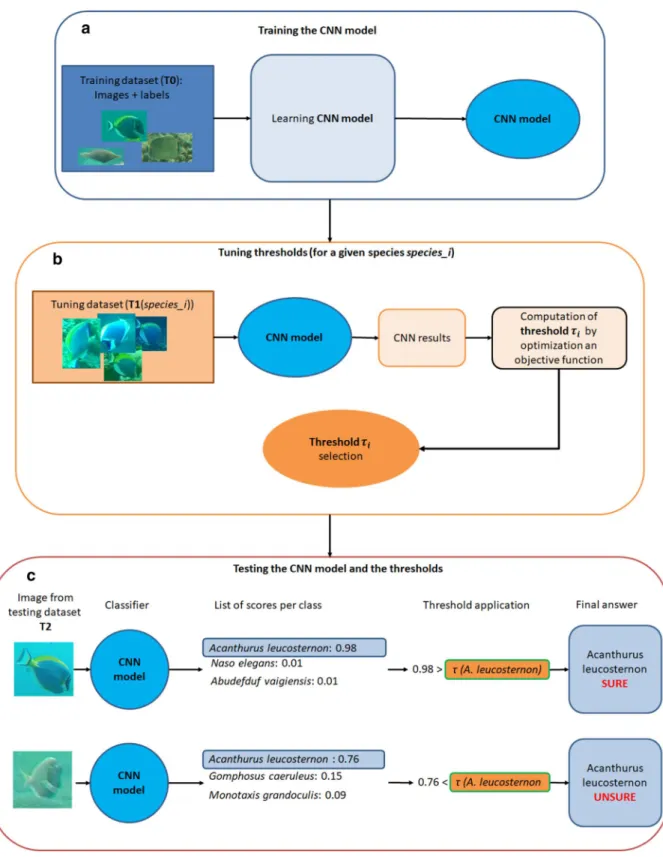
Figure 2. Overview of the 3 parts of our framework: 2 consecutive steps for the learning phase, followed by
the applicative testing step. (a) We trained a CNN model with a training dataset (T0) composed of images and a label for each image, in our case, the species corresponding to each fish individual. (b) Then, for each species i, we processed an independent dataset T1, with our model. For each image, we obtained the species j attributed by the CNN to the image and a classification score Sj . We have the ground truth and the result of the
classification (correct/incorrect), so we can define a threshold according to the user goal. This goal is a trade-off between the accuracy of the result and the proportion of images fully processed. (c) We then used this threshold to post-process outputs of the CNN model. More precisely, for a given image, the classifier of the CNN returns a score for each class (here for each fish species). The most likely class C(X) for this image is the one with the highest score S(X) We then compared this highest score S(X) with the computed confidence threshold for this species (τC(X)) obtained in the second phase. If the score was lower than the computed threshold that is
The question is now to select “optimal” thresholds {τi}i=ni=1 based on the dataset T1. This is not straightforward
as is it up to user specific objective, such as minimizing MC, maximizing CC, minimizing UC… In the following, we analyze three different goals corresponding to some standard protocols in marine ecology:
• The first goal G1 consists of keeping the best correct classification rate while reducing the misclassification error rate. For this, we used two steps. First, we identified the threshold(s) τ which maximizes CCi(τ ) . Since
several thresholds could reach this maximum, we get a set of threshold(s) Seg1 . Then, we selected the threshold
with the lower MCi(τ ) . This can be mathematically written as:
• The second goal G2 consists in constraining the misclassification error rate to an upper bound of 5% while maximizing the correct classification rate. Reaching this goal requires to first find Seg2 the set of threshold(s)
such as MCi(τ ) < 5%. If there is none, we considered Seg2 as the set of threshold(s), which minimize MCi .
Then we defined the optimal threshold τi by choosing the one in Seg2 which maximizes CCi:
• The third goal G3 consists of keeping the lowest misclassification rate while raising the correct classifica-tion error rate (implying a lower coverage). First, we defined Seg3 as the set of threshold(s) τ that minimizes
MCi(τ ) . If there were several thresholds with the same minimal value, we chose τi as the one which maximizes
CCi:
For a given image X in the test dataset, the classification and post-process is sequential as follows (Fig. 2c): (8) Seg1=arg max τ CCi(τ ) (9) τi=arg min τ′inSe g1 MCi τ′ (10) Seg2= τ/MCi(τ ) <5% (11) if Seg1= ∅then Seg2=arg min
τ MCi(τ ) (12) τi=arg max τ′inSe g2 CCi τ′ (13) Seg3=arg min τ MCi(τ ) (14) τi=arg max τ′inSe g3 CCi τ′
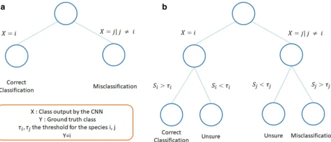
Figure 3. Impact of the post-processing framework on classification of images for a given species and a given
threshold. Usually, the classification of an image of class i can either be correct, if the model classifies it as i, or wrong, if the classifier classifies it as j with j = i (a). We propose a post processing to set a confidence threshold for each class to obtain 3 types of results, correct, misclassified, and unsure (b). The goal is then to transform as many misclassifications as possible as “Unsure”, while preventing to transform too many correct classifications “Unsure”.
• First, the image is given to the CNN, which outputs a list of scores, including S(X) the highest score obtained by a class.
• Second, for the class C(X) (i.e. the class with the highest classification score), the post-processing step esti-mates the risk of classifying the image as belonging to the class C(X) . If (X) < τj , the prediction is changed
to “Unsure”, otherwise, it is confirmed as the class j (Fig. 2c).
The misclassification rate for a species Y = i after post-processing thus equals:
and the unsure classification rate equals:
First, to assess the effectiveness of our framework, we processed all the images contained in T2 through the DL algorithm, without post processing (threshold tuning + threshold application).
Second, we assessed whether a unique threshold for all the classes was sufficient to separate correct classifica-tions from misclassificaclassifica-tions for all species. For this test, we computed the distribution of correct classificaclassifica-tions and misclassifications over scores for each species. During this study, we multiplied the softmax scores, which ranged from 0 to 1, by 100, for an easier reading.
Then, to study the impact of the post-processing method in an hypothetical ideal condition, we selected the thresholds based on the dataset T2 and we applied them to the same dataset T2. For this experiment and the following, we also measured both the Correct Classification rate and the Accuracy, defined for a species i as
The accuracy varies from 0 to 1, and increases when the number of false positives decreases and the number of true positives increases. Meanwhile, the CC rate varies from 0 to 100, and increases when the number of false negatives decreases and the number of true positives increases.
(15) MC′i= # (C(X) �= Y)AND S(X) > τj AND(Y = i) #(Y = i) (16) UC′i= # C(X) = j AND S(X) < τj AND(Y = i) #(Y = i) Accuracyi= #((C(X) = i)AND(S(X) > τi))AND(Y = i) #((C(X) = i)AND(S(X) > τi))
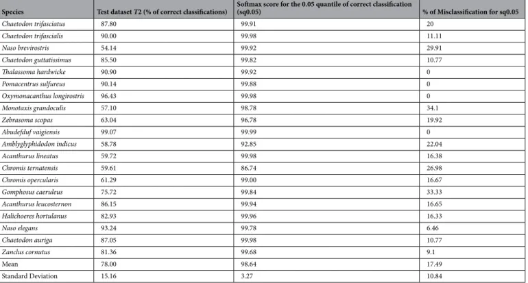
Table 1. Output of the deep learning classifier without post-processing. Percentages of correct classifications
are shown for the 20 fish species. Each line shows the species name, the correct classification rate of images of this species present in the dataset T2, the softmax score above which we have 95% of the correct classification (noted sq0.05), and the percentage of Misclassified images with score equal or above sq0.05.
Species Test dataset T2 (% of correct classifications) Softmax score for the 0.05 quantile of correct classification (sq0.05) % of Misclassification for sq0.05
Chaetodon trifasciatus 87.80 99.91 20 Chaetodon trifascialis 90.00 99.98 11.11 Naso brevirostris 54.14 99.92 29.91 Chaetodon guttatissimus 85.50 99.82 10.77 Thalassoma hardwicke 90.90 99.92 0 Pomacentrus sulfureus 90.14 99.88 0 Oxymonacanthus longirostris 96.43 99.98 0 Monotaxis grandoculis 57.10 98.78 34.1 Zebrasoma scopas 63.04 96.78 19.92 Abudefduf vaigiensis 99.07 99.99 0 Amblyglyphidodon indicus 58.78 92.85 22.04 Acanthurus lineatus 59.72 99.98 16.38 Chromis ternatensis 59.61 86.74 26.98 Chromis opercularis 61.29 99.00 16.67 Gomphosus caeruleus 75.72 99.84 33.33 Acanthurus leucosternon 86.15 99.94 16.65 Halichoeres hortulanus 82.93 99.96 16.33 Naso elegans 93.24 99.78 6.46 Chaetodon auriga 87.05 99.98 10.77 Zanclus cornutus 81.36 99.68 9.1 Mean 78.00 98.64 17.49 Standard Deviation 15.16 3.27 10.84
Figure 4. Distribution of correct classifications and misclassifications of fish images with respect to the score
from the CNN model. We plotted the results for all species (a), and for 2 species, the Brown unicornfish (Naso
brevirostris) (b) and the Maldives damselfish (Amblyglyphidodon indicus) (c). We also plotted the 5% bottom
line for each type of classification. We used violin plots for the visualisation. Violin plot are histograms with inverted axis allowing a graphical visualisation of a distribution, with the number of individuals on the Y axis and their value on X axis. The borders of the shapes show the number of individuals while the dots show the local density”46.
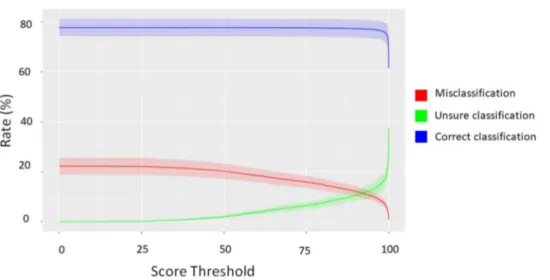
Figure 5. Average distribution of correct, wrong, and unsure classifications for all species along a gradient of
Finally, to ensure that the post-processing method was relevant for any real-life application, i.e. that thresh-olds are defined and tested on independent datasets, we used the dataset T1 for the threshold-setting phase and the dataset T2 for the testing phase. To assess the robustness of our method, we repeated the same experiment while switching the roles of T1 and T2. Note that we limited our experiments to the use of T1 and T2, but that it could be interesting in further work to assess the robustness of this method with datasets composed of less data.
Results
Results of the CNN model classification.
The mean rate of correct classification of fish images inT2 by the raw CNN was of 78.0%, with rates of correct classifications per species ranging from 54.4% to 99.1% (sd = 15.16) (Table 1). These results are the baseline for our following experiments.Images obtained softmax scores between 41 and 100 with 80% of images classified with a score between 60 and 100 (Fig. 4a). The distribution of correct classifications and misclassifications among scores was highly vari-able among species (Fig. 4b,c, Table 1).
Benchmark of the threshold fine-tuning method.
For each species i, we computed CCi , MCi , UCivalues while varying the threshold. We computed and applied the thresholds on T2, according to Eqs. 8–16. As the score varied from 0 to 99.9, the misclassification rate decreased to 0.9% (Fig. 5). This decrease was mainly compensated by the increasing rate of unsure classifications between 0 and 99.9 of classification scores.
Indeed, the rate of correct classifications experienced little variation along this distribution of threshold scores, remaining between 74 and 78% for threshold scores between 0 and 99.8 and decreasing to 61% for threshold scores > 99.8. However, correct, wrong, and unsure classification rates were highly variable among species (Sup-plementary Table S2).
For the first goal G1, we defined the thresholds (one per species) to minimize the misclassification with CCi=max CCi . We obtained a mean rate of 78% (standard deviation = 15.15%) of correct classifications, 10.81%
(s.d = 8.15%) of unsure classifications, and 11.19% (s.d = 9.58%) of misclassifications (Fig. 6a).
For the second goal G2, we maximized the correct classifications while constraining the misclassification error rate to an upper bound of 5% (if possible). We obtained a rate of 75.47% (s.d = 17.83%) of correct classifications, 17.88% (s.d = 14.22%) of unsure classifications, and 6.66% (s.d = 6.44%) of misclassifications.
Figure 6. Benchmark scenario and cross–validation classification rates. We compare results obtained by tuning
the thresholds on T2 and using T2 as a testing set (a) and real-life scenario obtained by tuning the thresholds on T1 and using T2 as a testing set (b). For sub-figure: From top to bottom, rates of correct classifications, misclassifications, and unsure classifications for each post-processing: (1) Goal 1: Minimizing misclassification with CCi=max CCi , (2) Goal 2: maximizing correct classifications under the constraint of having less than
5% of misclassifications, (3) Goal 3: maximizing correct classification with MCi=min MCi , (4) No
For the third goal G3, we maximized the number of correct classifications with MCi=min MCi . We obtained
a rate of 68.21% (s.d = 22.41%) of correct classifications, 29.71% (s.d = 22.14%) of unsure classifications, and 2.07% (s.d = 3.20%) of misclassifications, on average. Compared to the first goal, we decreased the rate of correct classifications by 8.9% and the rate of misclassifications by 2.6% (Supplementary Table S4).
The accuracy of the goals G1, G2, and G3 were, on average, higher than the raw accuracy (0.53) with respec-tively 0.72, 0.89 and 0.94 (Table 2).
The thresholds showed higher variations among species for G1, with values ranging from 33.46 to 99.97, than for G3 for which values ranged from 99.86 to 99.98 among the 20 species (Supplementary Tables S2, S3).
Application of the method.
For a real cross-validation experiment, thresholds were set using T2 and then applied on T1. The correct, wrong and unsure classification rates were very close (difference < 2.6%) to those obtained with the benchmark situation (Supplementary Table S5).The proposed post-processing was able to decrease the misclassification rate by at least 10.05%, for all goals, and 19.02% at most compared to the raw output of the Deep Learning model (Fig. 6b). The accuracy followed the same tendency, with an average accuracy for G1, G2 and G3 respectively equal to 0.74, 0.81 and 0.92 (Table 3).
Finally, we also performed the same experiment while switching T1 and T2 roles (Supplementary Tables S6, S7, S8). For each goal, the unsure classification rate was higher after the switch (+ 3.8% for G1, + 4.4% for G2, and + 8.9% for G3), implying lower scores were obtained in both correct classification (− 3.5%, − 5%, − 7.3%) and misclassification, with the exception of the 2nd goal (-0.2%, + 0.6%, − 1.6%).
Discussion
Biodiversity monitoring is experiencing a revolution with the emergence of new sensors (light, noise, image, environmental DNA) that generate massive datasets and require powerful and accurate treatment tools. Indeed, species misclassifications must be controlled and limited to avoid false negatives or absences i.e., missing species that are actually present and false positives or presences i.e., detecting species that are actually absent.
In this paper, we demonstrated that the risk of misclassification by CNN algorithms can be measured and controlled in a processing step to provide more accurate identification of species on pictures. Such post-processing can be applied with any classifier as long as the output is a vector of scores. Reducing the misclassifica-tion rate is at the detriment of the correct classificamisclassifica-tion rate and increases “unsure” classificamisclassifica-tions, which implies a low coverage and a greater human effort needed to identify unclassified individuals. Hence, there is a trade-off between a more secure (less misclassifications) or a more automatic (more classifications) method so species thresholds can be set according to the goal or priority of the study or the availability and time of experts. Here
Table 2. Accuracy of the models without post-processing, and with post processing according to our goals,
with thresholds tuned and applied on T2. Each line shows the result for a species, with: the species name, the accuracy of the model without post processing, and the accuracy of the model with post processing according to the 3 goals defined earlier.
Species RawAccuracy G1Accuracy G2Accuracy G3Accuracy
Abudefduf vaigiensis 0.51 0.65 0.9 0.97 Acanthurus leucosternon 0.61 0.69 0.87 0.96 Acanthurus lineatus 0.87 0.91 0.97 0.97 Amblyglyphidodon indicus 0.08 0.74 0.94 0.98 Chaetodon auriga 0.95 0.99 1 1 Chaetodon guttatissimus 0.16 0.84 0.95 0.98 Chaetodon trifascialis 0.97 0.87 0.95 0.96 Chaetodon trifasciatus 0.56 0.62 0.79 0.97 Chromis opercularis 0.68 0.8 0.96 1 Chromis ternatensis 0.01 0.44 0.79 0.9 Gomphosus caeruleus 0.24 0.31 0.54 0.72 Halichoeres hortulanus 0.51 0.59 0.8 0.93 Monotaxis grandoculis 0.77 0.81 0.96 0.99 Naso brevirostris 0.02 0.9 0.96 1 Naso elegans 0.89 0.92 0.97 0.97 Oxymonacanthus longirostris 0.36 0.46 0.89 0.85 Pomacentrus sulfureus 0.52 0.7 0.91 0.95 Thalassoma hardwicke 0.78 0.85 0.93 0.95 Zanclus cornutus 0.55 0.68 0.87 1 Zebrasoma scopas 0.61 0.7 0.81 0.81 Mean 0.53 0.72 0.89 0.94 Standard deviation 0.30 0.18 0.10 0.07
we define three main goals which represent archetypal study cases. The first goal, maximizing the correct clas-sification rate but not limiting misclasclas-sifications, can be applied when avoiding false negatives is more important than detecting false positives. This can be the case for monitoring invasive species, since the priority is to detect the first occurrence of such invasive individuals with potential deleterious consequences on native biodiversity and ecosystem functioning47 particularly on islands48,49. For instance, the Indo-Pacific predator lionfish (Pterois
volitans and P. miles) has invaded most reefs of the Western Atlantic and depleted many native prey populations,
and are starting to spread in the Eastern Mediterranean Sea12. To better anticipate the impact of such species,
eco-system mangers needs to be aware of the first occurrence on reefs and can thus accept having “false alarms”. The same constrains applies for detection particular or emblematic individuals, like Whale Sharks, through photo-identification50 where the primary goal is to avoid missing an occurrence. In both ecological cases, experts will
eventually validate the few false positive identifications of targeted organisms by the algorithm to discard them. The second goal, maximizing the correct classification rate while limiting misclassifications at 5% maximum per species, can be applied when avoiding false negatives and false positives are both important. This is the trade-off scenario that requires the least human effort and that can process massive datasets with few errors. It can be recommended to analyze long videos (> 2 h) for monitoring biodiversity metrics that are weakly influenced by undetected species (rare or classified as “unsure”), like the assessment of taxonomic or functional diversity25, and
that can feed initiatives like the Group on Earth Observations Biodiversity Observation Network (GEO BON) and provide robust estimates of Essential Biodiversity Variables (EBVs)3,4.
The third goal, minimizing the misclassification rate, can be applied when detecting false positives is more problematic than avoiding false negatives, which creates many “unsure” classifications. This can be the case when priority is to accurately analyze a relatively small dataset with the support of many experts who can help to identify species on potentially a high number of “unsure” images. For instance, assessing abundance of all species within a given area to explain ecosystem functioning (e.g.51) or to monitor changes in species relative
abundances (e.g.52) requires a minimum number of misclassifications.
Whatever the goal, our framework is highly flexible and can be adapted by tuning the species thresholds regulating the trade-off between classification robustness and coverage in an attempt to monitor biodiversity through big datasets where species are unidentified. To unclog the bottleneck of information extraction about organism forms, behaviors and sounds from massive digital data, machine learning algorithms, and particularly the last generation of deep learning algorithms, offer immense promises. Here we propose to help the users to control their error rates in ecology. This is a valuable addition to the ecologist’s toolkit towards a routine and robust analysis of big data and real-time biodiversity monitoring from remote sensors. With this control of error rate in the hands of users, Deep Learning Algorithms can be used for real applications, with acceptable and
Table 3. Accuracy of the model without post-processing, and with post processing according to our goals, on
the cross-validation, with thresholds tuned on T1 and applied on T2. Each line shows the result for a species, with: the species name, the accuracy of the model without post processing, and the accuracy of the model with post processing according to the 3 goals defined earlier.
Species RawAccuracy G1Accuracy G2Accuracy G3Accuracy
Abudefduf vaigiensis 0.51 0.61 0.92 0.97 Acanthurus leucosternon 0.61 0.7 0.92 0.94 Acanthurus lineatus 0.87 0.91 0.95 0.97 Amblyglyphidodon indicus 0.08 0.72 0.97 0.97 Chaetodon auriga 0.95 0.99 0.95 1 Chaetodon guttatissimus 0.16 0.88 0.72 0.96 Chaetodon trifascialis 0.97 0.9 0.96 0.98 Chaetodon trifasciatus 0.56 0.62 0.43 0.85 Chromis opercularis 0.68 0.83 0.03 1 Chromis ternatensis 0.01 0.47 0.97 0.87 Gomphosus caeruleus 0.24 0.31 0.89 0.75 Halichoeres hortulanus 0.51 0.57 1 0.9 Monotaxis grandoculis 0.77 0.82 0.99 0.98 Naso brevirostris 0.02 0.92 0.89 1 Naso elegans 0.89 0.91 0.99 0.97 Oxymonacanthus longirostris 0.36 0.46 0.72 0.8 Pomacentrus sulfureus 0.52 0.92 0.71 0.91 Thalassoma hardwicke 0.78 0.94 0.77 0.94 Zanclus cornutus 0.55 0.64 0.4 0.98 Zebrasoma scopas 0.61 0.66 0.99 0.8 Average 0.53 0.74 0.81 0.93 Standard deviation 0.30 0.19 0.25 0.07
controlled error rates, lower than any state of the art fully automatic process, while fixing the effort by human experts to correct algorithm mistakes.
Received: 21 October 2019; Accepted: 8 June 2020
References
1. Díaz, S. et al. Pervasive human-driven decline of life on Earth points to the need for transformative change. Science 366, 6471 (2019).
2. Schmeller, D. S. et al. Towards a global terrestrial species monitoring program. J. Nat. Conserv. 25, 51–57 (2015). 3. Pereira, H. M. et al. Essential biodiversity variables. Science 339(6117), 277–278 (2013).
4. Kissling, W. D. et al. Building essential biodiversity variables (EBVs) of species distribution and abundance at a global scale. Biol.
Rev. 93(1), 600–625 (2018).
5. Kröschel, M., Reineking, B., Werwie, F., Wildi, F. & Storch, I. Remote monitoring of vigilance behavior in large herbivores using acceleration data. Anim. Biotelem. 5(1), 10 (2017).
6. Steenweg, R. et al. Scaling-up camera traps: Monitoring the planet’s biodiversity with networks of remote sensors. Front. Ecol.
Environ. 15(1), 26–34 (2017).
7. Schulte to Bühne, H. & Pettorelli, N. Better together: Integrating and fusing multispectral and radar satellite imagery to inform biodiversity monitoring, ecological research and conservation science. Methods Ecol. Evol. 9(4), 849–865 (2018).
8. Wulder, M. A. & Coops, N. C. Make Earth observations open access: Freely available satellite imagery will improve science and environmental-monitoring products. Nature 513(7516), 30–32 (2014).
9. Hodgson, J. C. et al. Drones count wildlife more accurately and precisely than humans. Methods Ecol. Evol. 9(5), 1160–1167 (2018). 10. Koh, L. P. & Wich, S. A. Dawn of drone ecology: Low-cost autonomous aerial vehicles for conservation. Trop. Conserv. Sci. 5(2),
121–132 (2012).
11. Aguzzi, J. et al. Coastal observatories for monitoring of fish behaviour and their responses to environmental changes. Rev. Fish
Biol. Fish. 25(3), 463–483 (2015).
12. Mallet, D. & Pelletier, D. Underwater video techniques for observing coastal marine biodiversity: A review of sixty years of publica-tions (1952–2012). Fish. Res. 154, 44–62 (2014).
13. Robinson, D. P., Bach, S. S., Abdulrahman, A. A. & Al-Jaidah, M. Satellite tracking of whale sharks from Al Shaheen. QSci. Proc.
https ://doi.org/10.5339/qproc .2016.iwsc4 .52 (2016).
14. Cubaynes, H. C., Fretwell, P. T., Bamford, C., Gerrish, L., & Jackson, J. A. Whales from space: Four mysticete species described using new VHR satellite imagery. Mar. Mammal Sci. 35(2), 466–491 (2018).
15. Hodgson, A., Peel, D. & Kelly, N. Unmanned aerial vehicles for surveying marine fauna: Assessing detection probability. Ecol.
Appl. 27(4), 1253–1267 (2017).
16. Kellenberger, B., Marcos, D. & Tuia, D. Detecting mammals in UAV images: Best practices to address a substantially imbalanced dataset with deep learning. Remote Sens. Environ. 216, 139–153 (2018).
17. Francour, P., Liret, C. & Harvey, E. Comparison of fish abundance estimates made by remote underwater video and visual census.
Nat. Sicil 23, 155–168 (1999).
18. Chuang, M. C., Hwang, J. N. & Williams, K. A feature learning and object recognition framework for underwater fish images.
IEEE Trans. Image Process. 25(4), 1862–1872 (2016).
19. Marini, S. et al. Tracking fish abundance by underwater image recognition. Sci. Rep. 8(1), 1–12 (2018).
20. Joly, A. et al. Lifeclef 2017 lab overview: Multimedia species identification challenges. In International Conference of the
Cross-Language Evaluation Forum for European Cross-Languages 255–274. Springer, Cham (2017).
21. Li, X., Shang, M., Qin, H., & Chen, L. Fast accurate fish detection and recognition of underwater images with fast r-cnn. In
OCEANS’15 MTS/IEEE Washington 1–5. IEEE (2015).
22. Villon, S. et al. A deep learning method for accurate and fast identification of coral reef fishes in underwater images. Ecol. Inform.
48, 238–244 (2018).
23. Wäldchen, J. & Mäder, P. Plant species identification using computer vision techniques: A systematic literature review. Arch.
Comput. Methods Eng. 25(2), 507–543 (2018).
24. LeCun, Y., Bengio, Y. & Hinton, G. Deep learning. Nature 521(7553), 436 (2015).
25. Mouillot, D. et al. Rare species support vulnerable functions in high-diversity ecosystems. PLoS Biol. 11(5), e1001569 (2013). 26. Azzurro, E. & Bariche, M. Local knowledge and awareness on the incipient lionfish invasion in the eastern Mediterranean Sea.
Mar. Freshw. Res. 68(10), 1950–1954 (2017).
27. Gaston, K. J. What is rarity? In Rarity 1–21. (Springer, Dordrecht, 1994).
28. Chow, C. On optimum recognition error and reject tradeoff. IEEE Trans. Inf. Theory 16(1), 41–46 (1970).
29. Corbière, C., Thome, N., Bar-Hen, A., Cord, M., Pérez, P. Addressing Failure Prediction by Learning Model Confidence. arXiv e-prints https ://arXiv .org//arXiv :1910.04851 (2019).
30. Cortes, C., DeSalvo, G. & Mohri, M. Boosting with abstention. In Advances in Neural Information Processing Systems (eds Diet-terich, T. G. et al.) 1660–1668 (A Bradford Book, Cambridge, 2016).
31. Geifman, Y. & El-Yaniv, R. Selective classification for deep neural networks. In Advances in Neural Information Processing Systems (eds Dietterich, T. G. et al.) 4878–4887 (A Bradford Book, Cambridge, 2017).
32. De Stefano, C., Sansone, C. & Vento, M. To reject or not to reject: That is the question—An answer in case of neural classifiers.
IEEE Trans. Syst. Man Cybern. C 30(1), 84–94 (2000).
33. Kocak, M. A., Ramirez, D., Erkip, E., & Shasha, D. E. SafePredict: A meta-algorithm for machine learning that uses refusals to guarantee correctness. arXiv preprint https ://arxiv .org/1708.06425 (2017).
34. Niculescu-Mizil, A., & Caruana, R. Predicting good probabilities with supervised learning. In Proceedings of the 22nd international
conference on Machine learning 625–632. ACM (2005).
35. Guo, C., Pleiss, G., Sun, Y., & Weinberger, K. Q. On calibration of modern neural networks. In Proceedings of the 34th International
Conference on Machine Learning, Vol. 70, 1321–1330. JMLR.org. (2017)
36. Platt, J. Probabilistic outputs for support vector machines and comparisons to regularized likelihood methods. Adv. Large Margin
Class. 10(3), 61–74 (1999).
37. Zadrozny, B. & Elkan, C. Obtaining calibrated probability estimates from decision trees and naive Bayesian classifiers. Icml 1, 609–616 (2001).
38. Zadrozny, B., & Elkan, C. Transforming classifier scores into accurate multiclass probability estimates. In Proceedings of the eighth
ACM SIGKDD international conference on Knowledge discovery and data mining 694–699. ACM (2002).
39. Naeini, M. P., Cooper, G., & Hauskrecht, M. Obtaining well calibrated probabilities using bayesian binning. In Twenty-Ninth AAAI
Conference on Artificial Intelligence (2015).
40. Nixon, J. Dusenberry, M., Zhang, L. Jerfel, G. Tran, D. Measuring calibration in deep learning. In The IEEE Conference on Computer
41. Perez, L., & Wang, J. (2017). The effectiveness of data augmentation in image classification using deep learning. arXiv preprint
https ://arXiv .org/1712.04621 .
42. Goodfellow, I., Bengio, Y., Courville, A. & Bengio, Y. Deep Learning (MIT Press, Cambridge, 2016). 43. Abadi, M. et al. Tensorflow: A system for large-scale machine learning. OSDI 16, 265–283 (2016).
44. He, K., Zhang, X., Ren, S., & Sun, J. Deep residual learning for image recognition. In Proceedings of the IEEE Conference on Computer
Vision and Pattern Recognition 770–778 (2016).
45. Sarle, W. S. Stopped training and other remedies for overfitting. Computing Science and Statistics, 352–360 (1996). 46. Hintze, J. L. & Nelson, R. D. Violin plots: A box plot-density trace synergism. Am. Stat. 52(2), 181–184 (1998).
47. Catford, J. A., Bode, M. & Tilman, D. Introduced species that overcome life history tradeoffs can cause native extinctions. Nat.
Commun. 9(1), 2131 (2018).
48. Leclerc, C., Courchamp, F. & Bellard, C. Insular threat associations within taxa worldwide. Sci. Rep. 8(1), 6393 (2018). 49. Spatz, D. R. et al. Globally threatened vertebrates on islands with invasive species. Sci. Adv. 3(10), e1603080 (2017).
50. McKinney, J. A. et al. Long-term assessment of whale shark population demography and connectivity using photo-identification in the Western Atlantic Ocean. PLoS ONE 12(8), e0180495 (2017).
51. Maire, E. et al. Community-wide scan identifies fish species associated with coral reef services across the Indo-Pacific. Proc. R.
Soc. B Biol. Sci. 285(1883), 20181167 (2018).
52. Newbold, T. et al. Widespread winners and narrow-ranged losers: Land use homogenizes biodiversity in local assemblages world-wide. PLoS Biol. 16(12), e2006841 (2018).
Acknowledgements
We thank Emily S. Darling and Matthew J. McLean for taking on their time to comment our work, and help us to improve the manuscript, the GNUM for helping us to annotate the data and Clément Desgenetez who supported the annotation work. This work benefited from the Montpellier Bioinformatics Biodiversity platform supported by the LabEx CeMEB, an ANR "Investissements d’avenir" program (ANR-10-LABX-04–01). The CEMEB Labo-ratory of Excellency of Montpellier funded this study through a PhD grant to S Villon. NVidia supported this study by providing GPU device through the GPU Grant Program.
Author contributions
S.V. wrote the main manuscript text, prepared the figures, and carried the analysis. S.V., D.M., S.V., T.C., M.C., G.S. designed the project and the experiments. All authors reviewed the manuscript.
Competing interests
The authors declare no competing interests.
Additional information
Supplementary information is available for this paper at https ://doi.org/10.1038/s4159 8-020-67573 -7.
Correspondence and requests for materials should be addressed to S.V. Reprints and permissions information is available at www.nature.com/reprints.
Publisher’s note Springer Nature remains neutral with regard to jurisdictional claims in published maps and
institutional affiliations.
Open Access This article is licensed under a Creative Commons Attribution 4.0 International
License, which permits use, sharing, adaptation, distribution and reproduction in any medium or format, as long as you give appropriate credit to the original author(s) and the source, provide a link to the Creative Commons license, and indicate if changes were made. The images or other third party material in this article are included in the article’s Creative Commons license, unless indicated otherwise in a credit line to the material. If material is not included in the article’s Creative Commons license and your intended use is not permitted by statutory regulation or exceeds the permitted use, you will need to obtain permission directly from the copyright holder. To view a copy of this license, visit http://creat iveco mmons .org/licen ses/by/4.0/.