[Re] Non-Additive Coupling Enables Propagation of Synchronous Spiking Activity in Purely Random Networks

(1)

HAL Id: hal-01856930

https://hal.archives-ouvertes.fr/hal-01856930

Submitted on 13 Aug 2018

HAL is a multi-disciplinary open access

archive for the deposit and dissemination of

sci-entific research documents, whether they are

pub-lished or not. The documents may come from

teaching and research institutions in France or

abroad, or from public or private research centers.

L’archive ouverte pluridisciplinaire HAL, est

destinée au dépôt et à la diffusion de documents

scientifiques de niveau recherche, publiés ou non,

émanant des établissements d’enseignement et de

recherche français ou étrangers, des laboratoires

publics ou privés.

To cite this version:

Romain Cazé, Marcel Stimberg, Benoît Girard. [Re] Non-Additive Coupling Enables Propagation of

Synchronous Spiking Activity in Purely Random Networks. The ReScience journal, GitHub, 2018, 4

(1), �10.5281/zenodo.1246659�. �hal-01856930�

(2)

[Re] Non-additive coupling enables propagation of

synchronous spiking activity in purely random networks

Romain Cazé

1

_{, Marcel Stimberg}

2

_{, and Benoît Girard}

1

1 Sorbonne Université, ISIR équipe AMAC, Paris, France 2 Sorbonne Université, INSERM,

CNRS, Institut de la Vision, Paris, France romain.caze@upmc.fr Editor Nicolas P. Rougier Reviewers Pietro Marchesi Dennis Goldschmidt Received January 26, 2018 Accepted April 23 2018 Published May 12, 2018 LicenceCC-BY Competing Interests:

The authors have declared that no competing interests exist.

 Article repository

 Code repository

A reference implementation of

→ Non-additive coupling enables propagation of synchronous spiking activity in purely random networks, R.M. Memmesheimer, M. Timme, PLoS Computational Biology, 8(4): e1002384, 2012. DOI: 10.1371/journal.pcbi.1002384

Introduction

Dendritic non-linearities increase neurons’ computation capacity, turning them into

complex computing units [4]. However, network studies are usually based on point

neuron models that do not incorporate dendrites and their non-linearities. In

con-trast, the study replicated here [2] uses a simple point-neuron model that contains an

effective description of dendrites by a non-linear summation of its excitatory synaptic input. Due to the simplicity of the model, both large-scale parameter exploration of a medium-sized network, as well as an analytical investigation of its properties are feasible.

The original study was based on simulation and analysis code in C and Mathe-matica, but this code is not publicly available. Here, we replicate the study using the

neural simulator Brian 2 [1, 6], a simulator based on the Python language that has

become a common choice in computational neuroscience [3]. This simulator offers a

good trade-off between flexibility and performance and is therefore a suitable choice for this study of a non-standard neuron model.

Methods

Neural network model

The simulations in the original paper were done in phase representation, but our imple-mentation uses the more standard representation in terms of the neurons’ membrane

potential. The membrane potential Vi of neuron i, measured relative to the resting

potential, is described by:

τm dVi(t) dt =−Vi(t) + V0+ σ  ∑ j_∈Ei wexϵj(t− τ)   −∑ j_∈Ii winϵj(t− τ), (1)

where V (t) is the membrane voltage at time t, τm the membrane time constant, V0

(3)

and win respectively the excitatory and inhibitory weights, τ the transmission delay,

and Ei and Ii the indices of neurons that connect with respectively excitatory and

inhibitory weights to neuron i. If the membrane potential crosses a threshold Θ, it emits the spike and its membrane potential is reset to its resting potential, i.e. 0 mV.

The function ϵj is 1 whenever neuron j spikes, and 0 otherwise. Equation 1 is an

alternative, mathematically equivalent formulation of equation (1) of [2].

The originality of this model lays in a filtering of the excitatory inputs by the function σ to model dendritic non-linearities. The study considers two functions σ

(see Fig. 1 of the original paper and insets in Fig. 3). Linear coupling, defined by

σ(x) = x, and non-linear coupling with:

σ(x) =      x, if x≤ Va, Va+V_Vc_b_−V−V_aa(x− Va), if Va< x≤ Vb, Vc, otherwise. (2)

For this non-linear function, the biological interpretation is that below a first

thresh-old Va, excitatory inputs are propagated passively by the dendrite and sum linearly.

Above this threshold, they trigger a dendritic spike, resulting in an amplified somatic

voltage. If they are even higher and cross the threshold Vb, they stop increasing the

somatic voltage and saturate. Note that this non-linearity only affects spikes received

synchronously as has been observed experimentally [5]. With the introduction of this

non-linearity, the modelled point neuron becomes an effective model of a neuron with one non-linear dendrite.

The network consists of N neurons, where a directed synaptic connection between

a pair of neurons is established with probability p0. Each of these connections is

taken to be excitatory with probability pex, and inhibitory otherwise. Note that this

connection scheme implies that neurons cannot be separated into groups of excitatory and inhibitory neurons, a neuron typically projects with both excitatory and inhibitory connections to other neurons.

The parameter values used in the original study as well as in our replication are

summarised in Table1.

Parameter Symbol Value

Number of neurons N 1000

Connection probability p0 0.3

Probability connection being excitatory pex 0.5

Excitatory connection weight wex 0.2 mV (varied in Fig.2)

Inhibitory connection weight win 0.2 mV (varied in Fig.2)

Membrane time constant τm 8 ms

Firing threshold Θ 16 mV

External input V0 17.6 mV (effect on V )

Synaptic delay τ 5 ms (but see

Imple-mentation section)

Threshold for supra-linear summation Va 2 mV

Threshold for saturation Vb 4 mV

Saturation value Vc 6 mV

Table 1: Parameter values used in the simulations

Implementation and numerical methods

The authors of the original study provided us with the principal C and Mathematica code used in their study. However, this code does not compile and run any more with

(4)

recent Mathematica versions. Our implementation is not based on this code, but only on the descriptions in the original paper (with minor clarifications provided by the authors where necessary).

The authors of the original study used an event-based simulation scheme, exploiting the linearity of the sub-threshold dynamics. Due to this linearity, the membrane potential can be advanced for arbitrarily large time spans between spikes, and spike times do not have to be bound to any temporal grid. In contrast, the Brian simulator is built on a clock-driven paradigm where time is advanced in discrete steps. This is because the simulator supports a wide range of neural models of and event-driven methods can only be applied to a small number of simple neuron models, and also becomes computationally demanding in large networks with many spikes.

All simulations presented here have been performed with a step size of 0.1 ms and the forward Euler integration algorithm (changing to an exact integration based on the analytical solution of the linear equations did not change the results).

Note that the event-based method used in the original study has important conse-quences for the specific implementation of non-linear synaptic summation: only spikes that arrive exactly synchronously can sum up non-linearly. This, together with the synaptic delay that is constant over all connections, implies that the non-linearity will only apply to spikes that originate from neurons that spiked perfectly synchronously one synaptic delay earlier; randomly occurring spikes have only an infinitesimally small chance to arrive at the receiving neuron synchronously. When using a clock-driven algorithm, as we do in this replication, this is no longer the case. All neurons that spike within the same time step will deliver their spikes to their target neurons at the same time step, potentially triggering non-linear summation. While the clock-driven method is a less accurate method in general, we would argue that in the context of non-linear summation it is actually closer to the biological phenomenon it models.

While dendrites detect synchronous events with sub-millisecond precision [5], this

pre-cision is of course finite. With that said, the qualitative results of the original study can be replicated with a clock-driven method, as we will show in the Results section. For linearly coupled networks, the neuron model is a standard leaky-integrate-and-fire neuron with “delta synapses”, i.e. incoming synaptic events instantaneously affect the membrane potential as soon as they are received. In Brian, this model is described as follows (omitting the code to connect the synapses and set their weights):

eq = "dV/dt = -gamma*V + V0 : volt"

G = br2.NeuronGroup(N, model=eq, threshold="V>Theta", reset="V=0*mV", method='euler')

exc_syn = br2.Synapses(G, G, 'w : volt (constant, shared)', on_pre='V += w', delay=5 * ms - dt) inh_syn = br2.Synapses(G, G, 'w : volt (constant, shared)',

on_pre='V -= w', delay=5 * ms - dt)

Note that the delay has been set as one time step (dt) less than 5 ms. This is because in Brian, when a neuron receives synaptic input, this input can only trigger a threshold crossing of the receiving neuron in the following time step. To get chains of propagated synchronous spikes every 5 ms as in the original study, we therefore have to reduce the delay by one time step.

We used the predefined clip function to implement non-linear coupling in the network. The function clips a value to a given range, following the syntax

clip(value, lower_bound, upper_bound)

We employed this function on the received excitatory inputs stored in a placed

holder variable ve. The variable corresponds to x in eq.2. We then reset the variable

ve back to 0 to prepare for the next time step. In Brian syntax (the definition of the inhibitory synapses is identical to the linearly coupled network):

(5)

ve : volt """

G = br2.NeuronGroup(N, model=eq, threshold="V>Theta", reset="V=0*mV", method='euler')

exc_syn = br2.Synapses(G, G, 'w : volt (constant, shared)', on_pre='ve += w', delay=5 * ms - dt) G.run_regularly('''

V += clip(ve, 0*mV, 2*mV) + clip(2*(ve-2*mV), 0*mV, 4*mV) ve = 0*mV

''', when='after_synapses')

The run_regularly operation applies the non-linearity to the summed input at every time step.

In addition to random initial conditions, i.e. random initial values of the mem-brane potential, the simulation includes 1–50 random spikes “initially in transit”. The original article does not go into further details about their implementation, so we de-cided to use the following: at the beginning of the simulation, a uniformly distributed number between 1 and 50 is drawn to determine the total number of initial spikes. These spikes are “in transit”, meaning that they are modelled as arising from events before the start of the simulation. Since the synaptic delay in the network is 5 ms, we draw the arrival times for these spikes between 0 ms and 5 ms. Consistent with

the probability for excitatory connections in the network (pex = 0.5), we take half

of these spikes as arising from excitatory and half from inhibitory sources, modelling their effect as described above.

To facilitate simulation, we use the joblib library to automatically store results and to distribute computation over processor cores. Several simulation and analysis functions are annotated with a @mem.cache decorator, meaning that their input argu-ments and outputs will be automatically stored to disk and calling the function will return the stored values if available. This feature does not only ease development (e.g. plotting functions can be changed without re-running the underlying simulations), but also allows to interrupt long-running parameter explorations without losing the results obtained so far. The same result could be achieved by manually storing results to disk, but joblib’s caching mechanism helps to avoid common errors (e.g. to re-use an old result obtained with an outdated version of the code) while keeping the code readable.

To reduce the total simulation time, the grid exploration in Fig.2, and the analysis of

group size evolution in Fig.3have been distributed over processor cores using joblib’s

Parallel construct. For the simulations presented in Fig.2, multiple repetitions for

the same combination of synaptic weights are distributed over processor cores, for the

simulations presented in Fig.3, simulations are evaluated in parallel over group sizes.

In both cases, a number of C− 1 parallel processes is used, where C is the number of

processor cores in the user’s system.

We wanted reproducible simulations despite the use of random connectivity and initial conditions. Setting a single global seed was not sufficient because we used parallel simulations executed in non-deterministic order. Instead, we used a set of pre-determined seeds, one for each figure, and used those “meta-seeds” to generate a set of random seeds for each individual simulation.

For the grid search presented in Fig.2, we varied inhibitory and excitatory

synap-tic weights between 0.16 mV and 0.4 mV. Given that each neuron receives on average 150 excitatory and 150 inhibitory inputs, this corresponds to a “total weight” between

24 mV and 60 mV, as used on the axes of Fig.2. We used a resolution of 100 steps

for each variable, comparable to the 96 steps used in the original publication. Each network was simulated 10 times with different initial conditions (synaptic connec-tions and initial membrane potential values), whereas the original publication used 20 simulations per weight combination.

To numerically derive the evolution of synchronous pulse sizes presented in Fig.3

(6)

56 ms each. During each simulation, we stimulated the network at 50 ms with a syn-chronous pulse of activity, consisting of between 1 and 181 neurons (varied in steps of 5 – the original study used group sizes in the same range varied in steps of 6). We then observed the number of active neurons at 55 ms, i.e. at one τ after the stimula-tion. For each stimulation group size, we ran the simulations 50 times with different initial conditions, consistent with the original study. To achieve a better quantitative match with the original study, we applied a correction for the stimulation group size

g′₀ and the observed group size g₁′ in the next iteration (for the uncorrected results,

see Fig.7). We refer to the corrected values as ˆg0 and ˆg1, respectively. These

correc-tions are necessary because of the background activity and our clock-based simulation method and are motivated as follows. The activity of the full network in the absence

of stimulation is about 55 kHz (see Fig. 1). Given that our simulation uses a time

step of 0.1 ms, this means that at every time step about 5.5 neurons on average are

synchronously active. When we stimulate a network with a pulse of g′0 synchronous

neurons, the actual number of synchronously active neurons is therefore higher than this stimulation. Similarly, we have to correct the size of the observed group in the next iteration. In contrast to the simulation strategy of the original publication that could make use of an “infinite precision” to detect synchronous spikes triggered by the stimulation, our simulation will also detect all the synchronous spikes resulting from

the background activity. In the corrected values shown in Fig.3we therefore used the

actually observed synchronous spikes ˆg′₀≥ g₀′ at the time of the stimulation, and the

number of added spikes due to the stimulation ˆg′₁ = g_1stim′ − g′_{1no stim}, where g′_1stim

is the number of synchronous spikes we observe in a network with stimulation, and

g′_{1no stim} the number of observed spikes in a network without stimulation. Both net-works are simulated with the same random seed and therefore have the same network connectivity and the same initial conditions; the only difference lies in the presence or

absence of external synchronous stimulation. Note that the correction for ˆg′1 slightly

“overcorrects”, as it discards all spikes that are resulting from background activity, even those that also would have been triggered by the stimulation.

Semi-analytical and analytical methods

We did not attempt to replicate the analytical solution for the evolution of synchronous

pulses based on diffusion approximation (blue dots in Fig. 4 of [2]), since the original

publication did not give a detailed description of this approach. However, we replicate the semi-analytical work that was described in more detail.

To calculate the semi-analytical solutions for Fig.3, based on a numerical estimate

of the distribution P (V ), we proceeded as follows. First, we ran 2× 50 (once for

the linear, once for the non-linear network) simulations of 250 ms. Each of these simulations was randomly connected and had random initial conditions, but received no additional synchronous stimulation. The original study additionally simulated each of the 100 networks 10 times, with the same synaptic connectivity but differing in the initial conditions. We then binned all membrane potential values over all time steps

and neurons into 100 bins in the voltage interval [−Θ/8, Θ] to obtain an estimate of

P (V ), the distribution of the membrane potential. Note that the original study did

not further specify how P (V ) was estimated from the simulation results.

We then calculate the expected synchronous group size after one iteration as in the original publication. To make this calculation clearer, we now describe its derivation in detail. From the distribution P (V ) we can estimate the probability F that an additional input ϵ drives the neuron over its threshold (or equivalently, that the neuron is less than ϵ away from its threshold):

F (ϵ) = P (V > Θ− ϵ) =

∫ Θ

Θ_−ϵ

P (V )dV (3)

(7)

inhibitory spikes, i.e. ϵ(nex, nin) = σ(nexwex) + ninwin. Let us assume that in the

previous iteration gi neurons spiked and that these neurons are refractory now, i.e.

that N−gineurons are available to spike in this iteration. To calculate the probability

for a single (non-refractory) neuron j to spike in response to these gi neurons, we

will first calculate the probability that out of the gi neurons that spiked, exactly nex

neurons are connected with excitatory connections and ninneurons are connected with

inhibitory connections to neuron j. There are( gi

nex+nin

)

possibilities to chose nex+ nin

out of gineurons, and

(_n_ex_+n_in

nex

)

possibilities to divide these neurons into groups of size

nexand nin. This yields the total number of combinations c(gi, nex, nin):

c(gi, nex, nin) = ( gi nex+ nin )( nex+ nin nex ) = gi! nex!nin!(gi− nex− nin)! (4)

The probability that these selected nex neurons are actually connected via excitatory

connections to neuron j, that the nin neurons are actually connected via inhibitory

connections to neuron j, and that the remaining gi−nex−ninneurons are not connected

to neuron j is:

p(gi, nex, nin) = (p0pex)nex(p0pin)nin(1− p0)gi−nex−nin (5)

Finally, we need to sum these probabilities up over all possible values for nexand nin,

multiplying it with the probability that the generated input elicits a spike. This yields

the total probability Ps_(g

i) that a neuron j spikes in response to the activity of gi

neurons in the previous iteration:

Ps(gi) = gi ∑ nex=1 gi∑−nex nin=0 F(ϵ(nex, nin) ) c(gi, nex, nin)p(gi, nex, nin) (6)

In Fig. 3, we plot the expected value of spiking neurons during the next iteration,

given a certain initial synchronous pulse g_i′:

E(gi+1|gi = gi′) = (N− g′i)P

s_(g′

i) (7)

Results

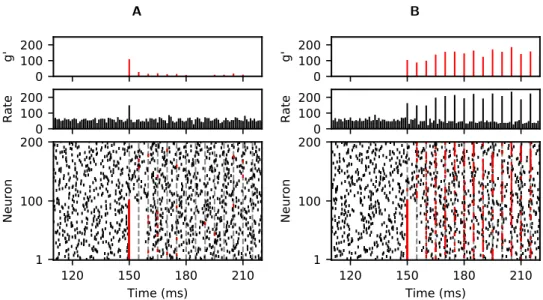
We first replicate a simulation showing the propagation of synchronous spiking activity

in networks using linear (Fig. 1A) and non-linear (Fig. 1B) coupling. This figure

corresponds to Fig. 2 of the original article. Given that the simulations are based on random synaptic connections and random initial conditions, we do not expect exact replication of spike times, but the qualitative features of the simulation are faithfully replicated: synchronous activity quickly dies out and disappears in the background

activity for linearly coupled networks (Fig.1A) but is persistently propagated in

non-linearly coupled networks (Fig.1B).

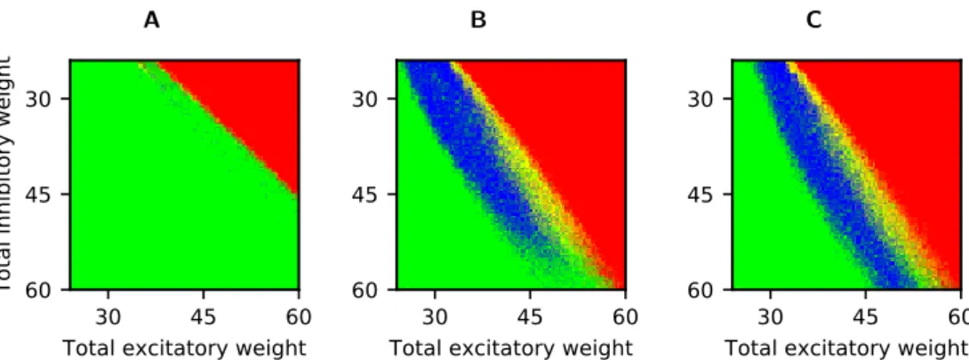
To confirm the equivalence of our network’s behaviour with the original study over a wide range of synaptic connection strength we ran a grid search exploration for

lin-early (Fig.2A) and non-linearly (Fig.2B) coupled networks. Network behaviour is

colour-coded as being part of one out of four classes: stable activity, but no persis-tent propagation (green); stable activity with persispersis-tent propagation (blue); unstable activity after synchronous stimulation (yellow); unstable activity before synchronous

stimulation (red). For quantitative definitions, see Table2. We run each combination

of connection strengths 10 times, and combine the results to yield a colour in RGB notation (values between 0 and 1 for the red, green, and blue component), according to:

(8)

A

0

100

200 g'

0

100

200 Rate

120

150

180

210 Time (ms)

1

100

200 Neuron

B

0

100

200 g'

0

100

200 Rate

120

150

180

210 Time (ms)

1

100

200 Neuron

Figure 1: Propagation of synchronous spiking in linearly (A) and non-linearly (B) coupled networks. We initiate a chain of synchronous pulses by applying external supra-threshold inputs

to the first 100 neurons at time t = 150 ms (red coloured spikes, grey vertical dotted lines indicate times where spikes occur as part of the chain). Top row: total size g′ of synchronised groups within the chain. Middle row: network rate over all neurons (rate in kHz, bin size 1 ms). Bottom row: spiking activity of the first 200 neurons in a network of a 1000 neurons versus time. Replication of Fig. 2 in [2] (https://doi.org/10.1371/journal.pcbi.1002384.g002).

Class Definition

U1 (red) Unstable before stimulation ∃t < tstim: ab(t)≥ 100

U2(yellow) Unstable after stimulation ∃t > tstim: ab(t)≥ 100

E (green) Stable activity, no propagation ∀t : ab(t) < 100 ∧ gp< 10

S (blue) Stable activity, persistent propagation ∀t : ab(t) < 100 ∧ gp≥ 10

Table 2: Classification of network behaviour for Fig.2. Here, abrefers to the background activity,

the number of neurons active during a 1 ms time bin, ignoring the time steps at tk

p = tstim+ k· τ,

i.e. time steps that follow the synchronous stimulation by multiples of the synaptic delay. The variable gp refers to the number of successful propagations of the synchronous activity, i.e. the

number of time steps tk

p where the number of active neurons exceeds the maximal background

activity ab.

where U1, and U2 stand for the fraction of trials displaying unstable network activity

before respectively after onset of propagation, and S and E for the fraction of trials displaying stable background activity with respectively without persistent propagation. We obtained this scheme directly from the authors of the original study, it was only coarsely described in the original publication. Combining individual results in this way does not necessarily lead to easily interpretable colours, but using a different scheme, e.g. colouring according to the class that occurred the most often, leads to visually

30

45

60 Total excitatory weight

30

45

60 Total inhibitory weight

B

30

45

60 Total excitatory weight

30

45

60

C

30

45

60 Total excitatory weight

30

45

60

Figure 2: Qualitative network behaviour as a function of excitatory and inhibitory connection strength for linearly (A) and non-linearly (B, C) coupled networks. For each combination,

we initiated synchronous activity with 100 (A, B) or 75 (C) neurons and assessed the stability of the temporal evolution. Blue colouring indicates stable propagation of synchrony, red indicates unstable background activity before onset of propagation, yellow indicates unstable background activity after onset of propagation, and green colouring indicates the absence of propagation (see Methods for details).

Replication of Fig. 3 in [2] (https://doi.org/10.1371/journal.pcbi.1002384.g003)

(red) happens for lower excitatory and higher inhibitory connection strength in our simulations than in the original article, i.e. that the red zone is shifted towards the bottom left. This is particularly evident for strong excitatory and inhibitory

connec-tions in non-linearly coupled networks (bottom right in Fig. 2B and C) which are

unstable in our simulations, but stable or only unstable after stimulation in the orig-inal publication. Simulating the parameter combination corresponding to the point

in the bottom right corner of the plot at different time resolutions (Fig. 6), we find

that this difference does indeed seem to be triggered by limited time resolution in the model. The forced synchronisation of all spikes to a grid of 0.1 ms, together with the homogeneity of the synaptic delays, leads to strong oscillations in our simulation

(Fig. 6A), which is consequently classified as unstable. When we use a simulation

time step of 0.01 ms, these oscillations disappear and the network activity therefore gets classified as “stable without persistent propagation”. Finally, non-linearly coupled networks show a discontinuity for weak inhibitory connection strengths in the original publication. For increasing excitatory connection strengths, network behaviour goes from stable (blue) to unstable after stimulation (yellow) to unstable before stimula-tion (red), but then get classified again as stable (blue) in a small range of parameters before finally transitioning to unstable activity (yellow and red). We do not observe

this in our simulations, but simulations with a finer time resolution (Fig.5C) indicate

that this difference could be caused by the limited time resolution of our simulations as well.

Despite these differences, the qualitative network behaviour looks very similar on a coarse scale. Importantly, it strongly supports the original paper’s main conclusion that non-linearly coupled networks have a large parameter range of stable propagation (i.e., blue-coloured points), while linearly coupled networks do not. The differences in our replication are most likely due to our use of a clock-based simulation method with

a limited time resolution (see Fig.5and Fig.6). In principle, another reason could be

implementation details of the initial “spikes in transit” that were not fully specified in the original article, but this seems unlikely since completely removing them did not change the results in a noticeable way (not shown).

Finally, we looked at the evolution of synchronous group sizes for one combination

of synaptic weights (wex= win= 0.2 mV) in detail (Fig.3). The results confirms our

previous conclusion that we can faithfully replicate the network behaviour which shows identical qualitative behaviour; the group size consistently declines with each iteration

(10)

A

1 25 50 75 100 125 150 175

# of synchronized neurons g

0₀

0

25

50

75

100

125

150

175 #

of

sy

nc

hr

on

ize

d

ne

ur

on

s g

0 1 B

1 25 50 75 100 125 150 175

# of synchronized neurons g

0₀

0

25

50

75

100

125

150

175 #

of

sy

nc

hr

on

ize

d

ne

ur

on

s g

0 1

Figure 3: Evolution of synchronous pulses in linearly (A) and non-linearly (B) coupled networks. To numerically estimate the probability distribution, we show occurrences of

pulse-sizes g′1 in response to a pulse of size g0′ by grey lines; green squares represent the corresponding

mean response group sizes.

Replication of Fig. 4 in [2] (https://doi.org/10.1371/journal.pcbi.1002384.g004)

in linearly coupled networks (Fig.3A), whereas it increases for intermediate group sizes

and declines otherwise in non-linearly coupled networks (Fig.3B). Quantitatively, the

semi-analytical results also match well. Based on the plotted values in the original

publication (Fig. 4 in [2]), the curve based on the semi-analytical solution crosses the

identity line at about 85 (G1) and 135 (G2) for non-linearly coupled networks, peaking

in between for g′₀≈ 125 and g′

1≈ 139. In our simulations, it crosses the line at about

86 and 134, and peaks at g₀′ ≈ 126 and g′

1 ≈ 137. As in the original article, our

numerical results show slightly lower values for the group size in the next iteration, with the biggest difference for values around the peak of the function for non-linearly

coupled networks (Fig. 3B). However, we see a quantitative difference for low initial

group sizes. In these simulations, the original publication shows a close match between the numerical results and the analytical solution. In our simulation, the semi-analytical solution overestimates the numerical one. Be reminded that to obtain this good quantitative match, we had to apply a correction to the numerical results, as

explained in the implementation section (for the uncorrected values, see Fig.7).

Despite the small quantitative differences, our work strengthens the original result by demonstrating a qualitative difference between linearly coupled and non-linearly coupled networks.

Discussion

We managed to qualitatively reproduce the main results of Raoul-Martin

Memmes-heimer and Marc Timme [2] despite some quantitative differences. The grid search

over parameters showed a higher prevalence of networks with unstable activity before the onset of stimulation compared to the original study. In the analysis of the evolu-tion of synchronous pulses of different sizes, our results need a correcevolu-tion for the use of a clock-based simulation method to show a good quantitative match with the orig-inal results. However, a marked difference remains for small initial group sizes. The differences we see are most likely due to our use of clock-based instead of event-driven simulations, as it forces all activity to a temporal grid of finite precision. However,

(11)

the main qualitative finding—non-linearly coupled networks have a large parameter range supporting persistent propagation of synchronous activity whereas linearly cou-pled networks do not—remains if we use finer (0.05 ms) or coarser (0.2 ms, 0.5 ms) temporal resolutions (data not shown).

The reusable code we provide with this work paves the way to future studies of networks of non-linearly coupled integrate-and-fire neurons. It gives researchers the means to verify that the original study’s conclusion hold under variations of its model assumptions, such as the details of the connectivity scheme or the synaptic model. This article has already provided a first such verification, demonstrating that the original studies main findings do not critically depend on the event-based method and the entailing “perfect time resolution”. Finally, we hope that the provided code can also serve as a basis for future studies of functional paradigms going beyond the mere propagation of synchronous activity.

Acknowledgements

We would like to thank Raoul Martin Memmesheimer for providing implementation details about the original study. This work has received funding from the European Union’s Horizon 2020 research and innovation programme under grant agreement No 640891 (DREAM Project).

References

[1] Dan F. M. Goodman and Romain Brette. “The Brian simulator”. In: Front. Neurosci. 3 (2009). doi:10.3389/neuro.01.026.2009.

[2] Raoul Martin Memmesheimer and Marc Timme. “Non-additive coupling enables propagation of synchronous spiking activity in purely random networks”. In: PLoS Computational Biology 8.4 (Apr. 2012). Ed. by Lyle J. Graham, e1002384. issn: 1553734X. doi:10.1371/journal. pcbi.1002384.

[3] Eilif Muller et al. “Python in neuroscience”. In: Front. Neuroinform. 9 (2015). issn: 1662-5196. doi:10.3389/fninf.2015.00011.

[4] Panayiota Poirazi, Terrence Brannon, and Bartlett W. Mel. “Pyramidal neuron as two-layer neural network”. In: Neuron 37.6 (Mar. 2003), pp. 989–999. issn: 0896-6273. doi:10.1016/ S0896-6273(03)00149-1.

[5] William Softky. “Sub-millisecond coincidence detection in active dendritic trees”. In:

Neuro-science 58.1 (Jan. 1994), pp. 13–41. issn: 0306-4522. doi:10.1016/0306-4522(94)90154-6. [6] Marcel Stimberg et al. “Equation-oriented specification of neural models for simulations.” In: Front. Neuroinform. 8.February (2014), p. 6. issn: 1662-5196. doi:10.3389/fninf.2014. 00006.

(12)

Supplementary Figures

A

30

45

60 Total excitatory weight

30

45

60 Total inhibitory weight

B

30

45

60 Total excitatory weight

30

45

60

C

30

45

60 Total excitatory weight

30

45

60

Figure 4: Most-often observed qualitative network behaviour as a function of excitatory and inhibitory connection strength All conventions as in Fig.2, but points are coloured according the observed qualitative behaviour that occurred the most often among the 10 independent simulations for given connection strengths.

A

35

40

45 Total excitatory weight

25

30 Total inhibitory weight

B

35

40

45 Total excitatory weight

25

30 Total inhibitory weight

C

35

40

45 Total excitatory weight

25

30 Total inhibitory weight

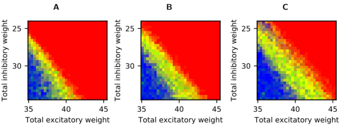
Figure 5: Zoom on qualitative network behaviour with different simulation time steps.

Colour code as in Fig.2. Results are shown for a smaller range of connection strengths than in Fig.2, and only for non-linearly coupled networks with an synchronous stimulation of 100 neurons. The total inhibitory connection strength was varied between 24 mV and 34.55 mV, the total excitatory connection strength was varied between 34.91 mV and 45.45 mV, i.e. the parameter range corresponds to a square region at the top of Fig.2B. Simulations where performed with simulation time steps of 0.1 ms (A; also the value used for all other simulations shown), 0.05 ms (B), and 0.01 ms (C).

(13)

A

0

100

200 g'

0

100

200 Rate

120

150

180

210 Time (ms)

1

100

200 Neuron

B

0

100

200 g'

0

100

200 Rate

120

150

180

210 Time (ms)

1

100

200 Neuron

Figure 6: Propagation of synchronous spiking in strongly connected networks when simu-lated with a time step of 0.1 ms (A), or 0.01 ms (B). All conventions as in Fig.1, but for strong recurrent connections (wex= win= 0.4 mV). Both simulated networks use non-linearly coupling,

the network shown in panel (B) is simulated with a 10-times finer temporal resolution compared to the other results shown.

A

1 25 50 75 100 125 150 175

# of synchronized neurons g

0₀

0

25

50

75

100

125

150

175 #

of

sy

nc

hr

on

ize

d

ne

ur

on

s g

0 1 B

1 25 50 75 100 125 150 175

# of synchronized neurons g

0₀

0

25

50

75

100

125

150

175 #

of

sy

nc

hr

on

ize

d

ne

ur

on

s g

0 1

Figure 7: Evolution of synchronous pulses without correction in linearly (A) and non-linearly (B) coupled networks. All conventions as in Fig.3. The numerical results shown here (grey lines and green squares) are not corrected for the bias introduced by the clock-driven integration method (see text for details).