Control of Hidden Mode Hybrid Systems: Algorithm termination
The MIT Faculty has made this article openly available.
Please share
how this access benefits you. Your story matters.
Citation
Verma, Rajeev and Domitilla Del Vecchio. "Control of Hidden Mode
Hybrid Systems: Algorithm Termination." 2011 14th International
IEEE Conference on Intelligent Transportation Systems Washington,
DC, USA. October 5-7, 2011.
As Published
http://dx.doi.org/10.1109/ITSC.2011.6083102
Publisher
Institute of Electrical and Electronics Engineers
Version
Author's final manuscript
Citable link
http://hdl.handle.net/1721.1/78371
Terms of Use
Creative Commons Attribution-Noncommercial-Share Alike 3.0
Control of Hidden Mode Hybrid Systems: Algorithm Termination
Rajeev Verma and Domitilla Del Vecchio
Abstract— We consider the problem of safety control in
Hidden Mode Hybrid Systems (HMHS) that arises in the development of a semi-autonomous cooperative active safety system for collision avoidance at an intersection. We utilize the approach of constructing a new hybrid automaton whose discrete state is an estimate of the HMHS mode. A dynamic feedback map can then be designed that guarantees safety on the basis of the current mode estimate and the concept of the capture set. In this work, we relax the conditions for the termination of the algorithm that computes the capture set by constructing an abstraction of the new hybrid automaton. We present a relation to compute the capture set for the abstraction and show that this capture set is equal to the one for the new hybrid automaton.
I. INTRODUCTION
The continuous advances of embedded computing and communication technologies are pushing most engineer-ing systems toward increased levels of autonomy. One such example is vehicles that can drive autonomously or semi-autonomously interacting with drivers and other human-driven vehicles. These technologies fall under In-telligent Transportation System initiatives of government and industry consortia. The availability of vehicle-to-vehicle (V2V) and vehicle-to-vehicle-to-infrastructure (V2I) wireless communication will bring these technologies one step closer to reality in the near future. For example, collision avoidance among multiple cars merging on an intersection is studied in [10]. The scheme employs a centralized control scheme that resides on the intersection and acts as a scheduler that assigns a safe time slot to each car for crossing the intersection.
While newer vehicles will be equipped with wireless radio to communicate and cooperate with other vehicles and the infrastructure, there will still be vehicles that will not be able to communicate. The control algorithms developed for guaranteeing safety must be able to operate in this partially autonomous real world scenario as long as road-side infrastructure (e.g., cameras, radar, and magnetic-induction loops) is employed to measure the approximate position of the non-communicating vehicles. This approach can be elegantly formulated as a safety control problem for hidden mode hybrid systems [20, 21]. The safety control problem for hybrid systems has been extensively considered in the literature when both the
R. Verma is with Electrical Engineering and Computer Science,
University of Michigan, Ann Arbor, USA{rajverma}@umich.edu
D. Del Vecchio is with the Department of Mechanical Engineering,
MIT, Cambridge, USA [email protected] Supported in part by NSF
CAREER Award Number CNS-0642719
continuous and discrete state are available for measure-ment [14, 16, 18, 19]. These measuremeasure-ments are required to compute a safe control input. In [1, 15], hybrid systems whose continuous dynamics is linear time-invariant and discrete state switching is due to transition guards are considered. An over approximation of the reachable set is computed using simulation techniques over bounded time in [15] and by using zonotopes in [1]. In [17], a hybrid system is considered whose discrete state can switch due to discrete control, discrete disturbance and discrete human input. Hybrid reachability results are then utilized to create an invariance-preserving discrete event system abstraction of the so called hybrid human-automation system. The knowledge of discrete input and perfect state information is assumed.
A number of works have addressed the control problem for special classes of hybrid systems with imperfect state information [5, 6, 24]. In [24], a controller that relies on a state estimator is proposed for finite state systems. The results are then extended to control a class of rectan-gular hybrid automata with imperfect state information, which can be abstracted by a finite state system. In [5–7, 11], computationally efficient state estimation and control algorithms were proposed for special classes of hybrid system with order-preserving dynamics. The problem of safety control for hidden mode hybrid systems has been addressed in [20, 21]. A perfect state information control problem is obtained by constructing a new hybrid automa-ton, whose discrete state is an estimate of the HMHS mode and is known. This problem is solved by computing the capture set and the least restrictive control map for the new hybrid automaton. Sufficient conditions for the termi-nation of the algorithm that computes the capture set are provided in [20, 21]. It has also been shown that the solved perfect state information control problem is equivalent to the original problem with imperfect state information under suitable assumptions. The main contribution of this paper is to show that in the case where the termination conditions for the algorithm that computes the capture set are not satisfied, an abstraction of the new hybrid automaton can be constructed for which the algorithm is guaranteed to terminate and such that the fixed point gives the capture set for the new hybrid automaton.
This paper is organized as follows. We recall some results from [20, 21] in Section II, the construction of the abstraction is shown in Section III and Section IV presents an application example.
II. Safety control problem for hidden mode hybrid systems
In this section, we summarize the results on safety control of HMHS from [20, 21]. We first present the general hybrid automaton model.
Definition 1. A Hybrid Automaton with Uncontrolled
Mode Transitions H is a tuple H = (Q, X, U, D, Σ, R, f ),
in which Q is the set of modes; X is the continuous state space; U is the continuous set of control inputs; D is the continuous set of disturbance inputs; Σ is the set of disturbance events that trigger transitions among modes; !∈ Σ is the silent event, which correspond to no transition occurring; R : Q× Σ → Q is the mode update map and
f : X×Q×U ×D → X is the vector field, which is allowed
to be piecewise continuous with its arguments.
For a hybrid automaton H, a hybrid time trajectory [16] is denoted by T = !N
i=0[τi, τ$i)] with σ(τ$i) ∈ Σ/!
and σ(t) = ! for t ∈ [τi, τ$i) for all i such that τi <
τ$i. Since the last interval may be open or closed (if
N < ∞), a “)]” parenthesis is used. We thus represent H by q(τi+1) = R(q(τ$i), σ(τ$i)), σ(τ$i) ∈ Σ/! and ˙x(t) =
f (x(t), q(t), u(t), d(t)), d(t)∈ D, σ(t) = !, where τi for i ∈
{0, ..., N} are the times at which a discrete transition takes place and satisfy τi≤ τ$i = τi+1, the value of q after the ith
transition is denoted by q(τi+1), q(t) := q(supτi≤tτi) for t∈
T and σ(t) = !, x(0) = x0∈ X, and q(τ0) = q0∈ Q. The
initial state x0 is known (the case where x0 is subject to
uncertainty is considered in [11]). We assume without loss of generality that τ0 = 0. The continuous state remains
the same after the discrete transition, i.e., x(τi+1) = x(τ$i)
for all i. For input signals u :T → U, d : T → D, σ : T → Σ, we denote the continuous trajectory of the system by x(t) = φx(t, (q0, x0), u, d, σ) for all t ≥ 0, in which
x(0) = φx(0, (q0, x0), u, d, σ) := x0 and the discrete state
trajectory by φq(t, q0,σ) = q(t) with q(0) = φq(0, q0,σ).
The set of reachable modes from any initial set of modes ¯q⊂ Q is denoted Rch(¯q) := !q0∈¯q!t≥0!σφq(t, q0,σ).
Definition 2. A Hidden Mode Hybrid System (HMHS)
is a hybrid automaton with uncontrolled mode transitions in which the discrete state q(t) is not measured and q0 is
only known to belong to a set ¯q0⊆ Q.
Thus, the mode of a HMHS is not known, the only measured state is x(t) and its evolution is driven by hidden mode transitions. In the remainder of the paper, we denote a HMHS by H. Let Bad⊆ X be a bad set of states. The control task is to keep the continuous state x(t) outside
Bad for all time using all the available information. The
available information at any time is the initial mode uncertainty, denoted ¯q0 ⊆ Q, the measured signals x(t)
and the control signal u(t).
Definition 3. A discrete state estimate is a time-dependent
set, denoted ˆq(t) ∈ ˆQ ⊆ 2Q, with the properties that (i)
q(t) ∈ ˆq(t) for all t ≥ 0; (ii) For t2 ≥ t1, we have that
ˆq(t2)⊆ Rch(ˆq(t1)).
Define the new hybrid automaton Hˆ = ( ˆQ, X, U, D, Y, ˆR, f ), in which ˆQ ⊆ 2Q is a new set
of discrete states, Y is a set of discrete events, ! ∈ Y is the silent event, ˆR : Qˆ × Y → ˆQ is a discrete state transition map. Let ˆT = !Nˆ
i=0[ˆτi, ˆτ$i)] be a hybrid
time trajectory such that ˆτ0 = τ0, y(ˆτ$i) ∈ Y/! and
y(t) = ! for t ∈ [ˆτi, ˆτ$i) for all i such that ˆτi < ˆτ$i. We
represent ˆH by ˆq(ˆτi+1) = ˆR( ˆq(ˆτ$i), y(ˆτ$i)), y(ˆτ$i)∈ Y/! and
˙ˆx(t) ∈ f ( ˆx(t), ˆq(t), u(t), d(t)), d(t) ∈ D, y(t) = !, where we have defined ˆq(t) := ˆq(supˆτi≤tˆτi) for all t∈ ˆT . Let the map
ˆ
R be such that ˆq(t) is a discrete state estimate, ˆx(0) = x0
and ˆq(ˆτ0) = ¯q0. Then, we refer to system ˆH as an
estimator. This in turn implies that (a) ˆR( ˆq, y)⊆ Rch(ˆq) for all y∈ Y and ˆq ∈ ˆQ and that (b) ˆτ$
0=ˆτ0=0 and y(ˆτ$0)
is such that ˆR( ˆq(ˆτ$0), y(ˆτ$0)) := Rch( ˆq(ˆτ0)) = Rch( ¯q0). The
discrete input y(t) derives information from the measured continuous state signal about the values of ˙x(τ) for τ < t and utilizes this information to determine the current set of modes compatible with such a derivative (see [3, 8, 9] for more information on mode estimators).
Since for system ˆH, the state ˆq(t) and ˆx(t) = x(t)
is measured, a safety control problem now becomes a problem with perfect state information. Specifically, given a feedback map u(t) = ˆπ( ˆq(t), ˆx(t)) for system ˆH, we
denote the closed loop system by ˆHˆπ. The flow of ˆHˆπ is
denoted by ˆφˆπ(t, ( ¯q
0, x0), d, y) and the continuous flow by
φˆπ
ˆx(t, ( ¯q0, x0), d, y). Also, a feedback map that guarantees
safety for ˆH also guarantees safety for H as the set of
trajectories of ˆH contain also those of H. For more details
on the relations between the solutions to the imperfect and the perfect information control problem, the reader is referred to [23]. The capture set for system H isˆ
given by ˆC := !ˆq∈ ˆQ " ˆq× ˆCˆq # , in which ˆCˆq := {x0 ∈ X| ∀ ˆπ, ∃ d, y, t ≥ 0 s.t. some φˆπ ˆx(t, ( ˆq, x0), d, y) ∈ Bad} is
called the mode-dependent capture set. It represents the set of all continuous states that are taken to Bad for all feedback maps when the initial mode estimate is equal to
ˆq.
Problem 1. (Control Problem with Perfect State
Infor-mation) Determine the set ˆC and a feedback map ˆπ that
keeps any initial condition ( ¯q0, x0)! ˆC outside ˆC.
The solution to Problem 1 can be obtained by leverag-ing results available for control of hybrid automata with perfect state information [20, 21]. For this purpose, for any ˆq∈ ˆQ and S ⊆ X define the operator Pre as Pre(ˆq, S ) := {x ∈ X | ∀ˆπ, ∃ d, t ≥ 0 s.t. some φˆπ
ˆx(t, ( ˆq, x), d, !) ∈ S }.
The set Pre( ˆq, S ) is the set of all continuous states that are taken to S for all feedback maps when the mode estimate is kept constant to ˆq.
A. Computation of the capture set
An algorithmic procedure is defined in [20, 21] for obtaining set ˆCˆq. We recall this procedure here. We use
for all ˆq∈ ˆQ the notation ˆR(ˆq, Y) := {ˆq$∈ ˆR(ˆq, y) | y ∈ Y},
in which we set ˆR( ˆq, y) := ∅ if ˆR(ˆq, y) is not defined for
some y∈ Y.
Definition 4. A set ˆW ⊆ ˆQ× X is termed a controlled
in-variant set for ˆH if there is a feedback map ˆπ such that for
all ( ¯q0, x0)∈ ˆW, we have that all flows ˆφˆπ(t, ( ¯q0, x0), d, y)∈
ˆ
W for all t, d, and y. A set ˆW ⊆ ˆQ× X is the maximal
controlled invariant set for ˆH provided it is a controlled
invariant set for ˆH and any other controlled invariant set
for ˆH is a subset of ˆW.
The next result (Proposition 1 of [20]) states that the complement of the capture set is the maximal controlled invariant set for ˆH.
Proposition 1. The set ˆW := ( ˆQ× X)/ ˆC is the maximal
controlled invariant set for ˆH contained in ( ˆQ× X)/( ˆQ ×
Bad).
Let ˆQ = {ˆq1, ..., ˆqM} with ˆqi ∈ 2Q for i ∈ {1, . . . , M},
Si∈ 2X for i∈ {1, . . . , M}, and define S := (S1, . . . , SM)⊆
(2X)M. We define the map G : (2X)M→ (2X)M as
G(S ) :=
Pre"ˆq1,!{ j| ˆqj∈ ˆR(ˆq1,Y)}Sj∪ Bad
# ..
.
Pre"ˆqM,!{ j| ˆqj∈ ˆR(ˆqM,Y)}Sj∪ Bad
# . Algorithm 1. S0:= (S0 1, S 0 2, . . . , S 0 M) := (∅, . . . , ∅), S1=G(S0) while Sk−1" Sk Sk+1=G(Sk) end.
If Algorithm 1 terminates, that is, if there is a K∗such that SK∗ = (SK∗ 1 , ..., SK ∗ M) = (SK ∗+1 1 , ..., SK ∗+1 M ) = SK ∗+1 , we denote the fixed point by S∗. It can be shown that if Algorithm 1 terminates, the fixed point S∗ is such that
S∗=( ˆCˆq1, ..., ˆCˆqM) (see Theorem 1 of [20]).
B. The control map
To determine the set of feedback maps that keep the complement of ˆC invariant, we employ notions from
viability theory [2].
Definition 5. A set-valued map F : X → 2X is said to
be piecewise Lipschitz continuous on X if it is Lipschitz continuous on a finite number of sets Xi ⊂ X for i =
1, ..., N that cover X, that is,!Ni=1Xi=X, and Xi∩ Xj=∅
for i" j.
Let X be a normed space and let S ⊂ X be nonempty. The contingent cone to S at x ∈ S is the set given by TS(x) := {v ∈ S | lim infh→0+dS(x+h v)h = 0}, in
which dS(y) denotes the distance of y from set S , that
is, dS(y) := infz∈K1y − z1. The next result (Proposition 6 of
[20]) extends conditions for set invariance as found in [2] to the case of piece-wise Lipschitz continuous set-valued maps. This extension is required in our case because the vector field f is allowed to be piece-wise continuous.
Proposition 2. Let F : X→ 2X be a set-valued Marchaud
map. Assume that F is piecewise Lipschitz continuous on X. A closed set S ⊆ X is invariant under F if and only if
F(x)⊆ TS(x) for all x∈ S .
For simplifying notation, for each mode ˆq∈ ˆQ define the set-valued map ¯f : X× ˆQ × U → 2X as ¯f( ˆx, ˆq, u) =
{ ˆf( ˆx, ˆq, u, d), d ∈ D} for all ( ˆx, ˆq, u) ∈ X × ˆQ × U. Define
Lˆq:= X\ ˆCˆqfor all ˆq∈ ˆQ and consider the set-valued map
defined as
Π( ˆq, ˆx) :={u ∈ U | ¯f( ˆx, ˆq, u) ⊂ TLˆq( ˆx)}. (1)
The following theorem (Theorem 3 of [20]) states that a control map can be selected that makes the complement of the capture set controlled invariant.
Theorem 1. Assume that ˆπ : ˆQ× X → U is such that
for all ˆq∈ ˆQ the set-valued map F( ˆx, ˆq) := ¯f ( ˆx, ˆq, ˆπ( ˆx, ˆq)) is Marchaud and piecewise Lipschitz continuous on X. Then, the set ( ˆQ× X)\ ˆC is invariant for ˆHˆπif and only if
ˆπ( ˆq, ˆx)∈ Π(ˆq, ˆx).
III. Termination of Algorithm 1
For the termination of Algorithm 1, sufficient condi-tions on ˆH are provided in [20]. For the systems that
do not satisfy these conditions, we show that one can construct an abstraction of ˆH for which Algorithm 1
always terminates and such that the fixed point gives the mode-dependent capture sets of ˆH. In order to proceed,
we introduce the notion of kernel sets for ˆH.
Definition 6. (Kernel set) The kernel set corresponding
to a mode ˆq∗ ∈ ˆQ is defined as ker( ˆq∗) :={ˆq ∈ ˆQ | ˆq ∈ ˆ
Rch( ˆq∗) and ˆq∗∈ ˆRch( ˆq)}.
The kernel set for a mode ˆq∗ is thus the set of all modes that can be reached from ˆq∗ and from which ˆq∗ can be reached. One can verify that for all pairs of modes ˆqi, ˆqj ∈ ˆQ, we have that ˆqi ∈ ˆRch( ˆqj) and ˆqj ∈ ˆRch( ˆqi)
if and only if ker( ˆqi) = ker( ˆqj). The next result shows
that any two modes of ˆH in the same kernel set have the
same mode-dependent capture set and hence the same set of safe feedback maps.
Proposition 3. For every kernel set ker⊆ ˆQ and for any
two modes ˆq, ˆq$∈ ker, we have that ˆCˆq = ˆCˆq$ and hence
that Π( ˆq, x) = Π( ˆq$, x).
Proof. Since ˆq, ˆq$ ∈ ker, we have that ˆq$ ∈ Rch( ˆq)ˆ and that ˆq ∈ Rch( ˆqˆ $). By Proposition 4 of [20], the
first inclusion implies that ˆCˆq$ ⊆ ˆCˆq, while the second
inclusion implies that ˆCˆq ⊆ ˆCˆq$. Hence, we must have
that ˆCˆq = ˆCˆq$. By equation (1), this in turn implies also
LetK := {ker(ˆq1), . . . , ker( ˆqM)}. Let there be p distinct
elements in K denoted ker1, . . . , kerp. Note that keri ∩
kerj=∅, for i " j. If each of the kernel sets is just one
element in ˆQ, it means that there are no discrete transitions
possible in ˆR that bring a discrete state ˆq back to itself.
That is, there is no loop in any of the trajectories of ˆq. In this case, one can verify that Algorithm 1 terminates in a finite number of steps (see [20]). If there are loops, then the existence of a maximal element in each kernel set guarantees termination, as has been shown in Theorem 2 of [20]. However, when not all kernel sets have a maximal element, this result does not hold. Hence, we propose a different approach based on constructing an abstraction of ˆH that merges all the modes that belong to the same
kernel set in a unique new mode.
Definition 7. Given hybrid system Hˆ =
( ˆQ, X, U, D, Y, ˆR, ˆf), the abstraction ˜H = ( ˜Q, X, U, D, ˜Y, ˜R,
˜
f ) is a hybrid system with uncontrolled mode transitions
such that
(i) ˜Q ={˜q1, ..., ˜qp}, ˜Y is such that ! ∈ ˜Y and ˜R(˜q, !) = ˜q
for all ˜q∈ ˜Q;
(ii) for all i, j ∈ {1, ..., p} there is ˜y ∈ ˜Y such that ˜qi =
˜
R( ˜qj, ˜y) if and only if there are ˆq$ ∈ keri, ˆq ∈ kerj,
and y∈ Y such that ˆq$= ˆR( ˆq, y);
(iii) for all i ∈ {1, ..., p}, x ∈ X, d ∈ D, and v ∈ U, we have that ˜f(x, ˜qi, v, d) :=!ˆq∈keri ˆf(x, ˆq, v, d).
Since p≤ m, the number of discrete states in system ˜
H is always less than or equal to that of system ˆH.
For a feedback map ˜π : Q˜ × X → U, initial states
x0 ∈ X and ˜q0 ∈ ˜Q, and signals ˜y, d, we denote the
flows of the closed loop system ˜H˜π by φ
˜q(t, ˜q0, ˜y) and
φ˜π
˜x(t, ( ˜q0, x0), d, ˜y), in which ˜x(t) := φ˜π˜x(t, ( ˜q0, x0), d, ˜y)
sat-isfies ˙˜x(t) ∈ ˜f( ˜x(t), φ˜q(t, ˜q0, ˜y), ˜π(φ˜q(t, ˜q0, ˜y), ˜x), d(t)). We
also denote by ˜C˜qi for i ∈ {1, ..., p} the mode-dependent
capture sets of ˜H. For any ˜q∈ ˜Q, we define ker( ˜q) := keri
provided ˜q = ˜qi. Also, for all ˜q∈ ˜Q, we denote the set of
reachable modes from ˜q as Rch( ˜q) :=˜ !t≥0!˜yφ˜q(t, ˜q, ˜y).
In the sequel, we denote ˜R( ˜q, ˜Y) :=!˜y∈ ˜YR( ˜q, ˜y), in which˜
we set ˜R( ˜q, ˜y) := ˜q if ˜R( ˜q, ˜y) is not defined for some ˜y∈ ˜Y. The following proposition is a direct consequence of the fact that all kernel sets of ˜H are singletons and there is
no loop in any of the trajectories of ˜q.
Proposition 4. Algorithm 1 terminates for system ˜H.
The next result shows that any piece-wise continuous signal, which is continuous from the right and contained in
ker(φ˜q(t, ˜q0,˜y)) is a possible discrete flow of ˆH for suitable
y starting from some ˆq0∈ ker(˜q0).
Proposition 5. For any piece-wise continuous signal α
that is continuous from the right and such that α(t) ∈
ker(φ˜q(t, ˜q0, ˜y)), there are ˆq0 ∈ ker(˜q0) and y such that
α(t) = φˆq(t, ˆq0, y) for all t.
Proof. Since α(t) ∈ ker(φ˜q(t, ˜q0, ˜y)) for all t, there are
times t0, ..., tN ≤ t and a sequence j0, ..., jN ∈ {1, ..., p}
such that α(t) ∈ kerji for all t ∈ [ti, ti+1). Since any
mode in kerji can transit to any other mode in kerji
instantaneously under the discrete transitions of ˆH, we
have that there are ˆqo,i ∈ kerji and yi such that α(t) =
φˆq(t− ti, ˆqo,i, yi) for all t ∈ [ti, ti+1). Also, for any two
modes αi ∈ kerji and αi+1 ∈ kerji+1 we have that αi+1 ∈
ˆ
Rch(αi). Hence, let α−i := limt→t−
i+1φˆq(t− ti, ˆqo,i, yi) and
α+
i := limt→t+
i+1φˆq(t− ti+1, ˆqo,i+1, yi+1). Then, since multiple
transitions are possible in ˆH at the same time, there is a
signal yi,i+1 such that α+i = φˆq(0, α−i, yi,i+1). Hence, there
is a signal y such that α(t) = φˆq(t, ˆqo,0, y) for all t. !
Theorem 2. For all kernel sets keriwith i∈ {1, ..., p} and
for all ˆq∈ keri, we have that ˆCˆq= ˜C˜qi.
Proof. Let ˆq∈ keri. We first show that ˆCˆq⊆ ˜C˜qi. Let x0 ∈
ˆ
Cˆq, then for all ˆπ : ˆQ× X → U, there are y, d, and t > 0
such that φˆπ
ˆx(t, ( ˆq, x), d, y)∈ Bad. This is in particular true
for all those feedback maps ˆπ such that ˆπ( ˆq, x) = ˆπ( ˆq$, x) whenever ˆq, ˆq$ ∈ kerj for some j ∈ {1, ..., p}. Hence, we
also have that for all ˜π : ˜Q× X → U, there are y, d, and t > 0 such that ˆx(t) := φ˜π
ˆx(t, ( ˆq, x), d, y) ∈ Bad, in
which ˙ˆx∈ ˆf( ˆx(t), φˆq(t, ˆq, y), ˜π(α(t), x(t)), d(t)) with α(t) :=
˜qj if φˆq(t, ˆq, y) ∈ kerj. Such a signal ˆx(t) also satisfies
˙ˆx ∈ ˜f( ˆx(t), α(t), ˜π(α(t), x(t)), d(t)) by the definition of ˜f. By the definition of ˜R, there is ˜y such that α(t) = φ˜q(t, ˜qi, ˜y)
for all t. Hence, ˆx(t) is also a continuous flow of ˜H starting
at ( ˜qi, x0) and therefore x0∈ ˜C˜qi.
We now show that C˜˜qi ⊆ Cˆˆq. If x0 ∈ C˜˜qi,
then for all feedback maps ˜π : Q˜ × X → U,
there are ˜y, d, and t > 0 such that ˜x(t) := φ˜π
˜x(t, ( ˜qi, x0), ˜y, d) ∈ Bad. Here, we have that ˜x(t)
satisfies ˙˜x(t) ∈ ˜f( ˜x(t), φ˜q(t, ˜qi,˜y), ˜π(φ˜q(t, ˜qi,˜y), ˜x), d(t)),
which is equivalent (by the definition of f ) to˜
˙˜x(t) ∈ ˆf( ˜x(t), ker(φ˜q(t, ˜qi,˜y)), ˜π(φ˜q(t, ˜qi,˜y), ˜x), d(t)), which
is equivalent to ˙˜x(t) = ˆf( ˜x(t), α(t), ˜π(φ˜q(t, ˜qi,˜y), ˜x), d(t))
for piece-wise continuous signal α (continuous from the right) such that α(t) ∈ ker(φ˜q(t, ˜qi,˜y)). By Proposition 5,
any such α(t) is such that there are y and ˆq0 ∈ ker(˜qi)
such that α(t) = φˆq(t, ˆq0, y) for all t, that is, it is a discrete
flow of system ˆH. Hence, for all π$ : ˆQ× X → U with ˆπ$( ˆq, x) = ˆπ$( ˆq$, x) for all ˆq, ˆq$∈ kerj for all j, there are
y, d, ˆq0 ∈ keri, such that φˆπ
$
ˆx(t, ( ˆq0, x0), y, d) ∈ Bad. By
Proposition 3, this implies that for all π : ˆQ×X → U there are y, d, ˆq0 ∈ keri, such that φˆπˆx(t, ( ˆq0, x0), y, d) ∈ Bad.
Hence, x0 ∈ ˆCˆq0. !
The above theorem can be utilized to compute the capture set of ˆH by constructing the abstraction ˜H and
ap-plying Algorithm 1 to it, which is guaranteed to terminate for ˜H. The next two technical propositions provide a
char-acterization of the Pre operator computed for system ˜H
and the relationship between ˜R and R. Specifically, denote
Prea( ˜q, S ) :={x0 ∈ X | ∀ ˜π ∃ t, d, s.t. φ˜π˜x(t, ( ˜q, x0), d, !)∈
S}.
Proposition 6. For all ˜q∈ ˜Q and S ⊆ X, we have that
Prea( ˜q, S ) = Pre(*ker( ˜q), S ).
Proof. From the definition of Prea( ˜q, S ), we have that x0 ∈ Prea( ˜q, S ) if and only if for all ˜π, there
are t, d such that ˜x(t) = φ˜π
˜x(t, ( ˜q, x0), d, !) ∈ S ,
in which ˙˜x(t) ∈ ˜f( ˜x(t), ˜q, ˜π( ˜x(t)), d(t)), which, by the definition of ˜f and of fˆ is equivalent to ˙˜x(t) ∈ f ( ˜x(t),!ˆq∈ker(˜q)!q∈ˆqq, ˜π( ˜x(t)), d(t)) =
f ( ˜x(t),*ker( ˜q), ˜π( ˜x(t)), d(t)). Hence, by the definition
of Pre, we have that x0 ∈ Prea( ˜q, S ) if and only if
x0∈ Pre(*ker( ˜q), S ). !
Proposition 7. Let ˜qj1, ˜qj0 ∈ ˜Q. If ˜qj1 ∈ ˜R(˜qj0, ˜Y) then
*ker( ˜q
j1)⊆ Rch(*ker( ˜qj0)).
Proof. If ˜qj1 ∈ ˜R(˜qj0, ˜Y), then by the definition of ˜R there
are ˆq∈ ker(˜qj0) and ˆq$ ∈ ker(˜qj1) such that ˆq$ = ˆR( ˆq, y)
for some y∈ Y. By the definition of a kernel set, this also implies that for all ˆq∈ ker(˜qj0) and ˆq$∈ ker(˜qj1), there is a
sequence of events y1, ..., yk and of modes ˆqj0, ..., ˆqjk ∈ ˆQ
such that ˆqj0 = ˆq, ˆqjk = ˆq$ and ˆqji+1 = ˆR( ˆqji, yi+1) for
i ∈ {0, ..., k − 1}. Since ˆR(ˆq, y) ⊆ Rch(ˆq) for all y ∈ Y and ˆq ∈ ˆQ, this in turn implies that ˆqji+1 ⊆ Rch(ˆqji) for
i ∈ {0, ..., k − 1}. This leads to ˆq$ ⊆ Rch(ˆq) for all ˆq ∈
ker( ˜qj0) and ˆq$ ∈ ker(˜qj1). This also implies that ˆq$ ⊆
Rch(*ker( ˜qj0)) and hence (since this holds for all ˆq$ ∈
ker( ˜qj1)) to*ker( ˜qj1)⊆ Rch(*ker( ˜qj0)). !
Lemma 1. For all ¯q ∈ Q, we have thatˆ Cˆ¯q =
Pre(Rch( ¯q), Bad).
Proof. First, we show that Cˆ¯q ⊆ Pre(Rch(¯q), Bad).
Since Algorithm 1 terminates in a finite number
n of steps for H, we have that˜ C˜˜q = Prea( ˜q,
! ˜qj1∈ ˜R(˜q, ˜Y)Prea " ˜qj1,!˜qj2∈ ˜R(˜qj1, ˜Y)Pre a"˜q j2, ..., ! ˜qjn−1∈ ˜R(˜qjn−2, ˜Y) Prea( ˜qjn−1, Bad)... ### . By
Proposition 6, we also have that C˜˜q =
Pre"*ker( ˜q),!˜qj1∈ ˜R(˜q, ˜Y)Pre"*ker( ˜qj1),!˜qj2∈ ˜R(˜qj1, ˜Y)
Pre"*ker( ˜qj2), ...!˜qjn−1∈ ˜R(˜qjn−2, ˜Y)Pre(*ker( ˜qjn−1), Bad)...
### . By Proposition 7, we have that *ker( ˜qj1) ⊆
Rch(*ker( ˜q)) and that *ker( ˜qji+1) ⊆ Rch(
*ker( ˜q
ji))
for i < n. Since the Pre operator and Rch preserve the inclusion relation in the first argument, these imply that ˜C˜q ⊆ Pre(Rch(*ker( ˜q)), Bad). Since for all
¯q1, ¯q2 ∈ ker(˜q) we have that Rch(¯q1) = Rch( ¯q2), we also
have that Rch( ¯q) = Rch(*ker( ˜q)) for all ¯q ∈ ker(˜q).
Hence, ˜C˜q ⊆ Pre(Rch(¯q), Bad) for all ¯q ∈ ker(˜q). This
along with Theorem 2 finally imply that for all ¯q∈ ker(˜q) we have ˆC¯q⊆ Pre(Rch(¯q), Bad).
To show that ˆC¯q ⊇ Pre(Rch(¯q), Bad), we employ the
properties of the Pre operator and Proposition 4 of [20]. By such a proposition, by the fact that (since ˆH is derived
from H) for all ¯q∈ ˆQ there is y ∈ Y such that ˆR(¯q, y) =
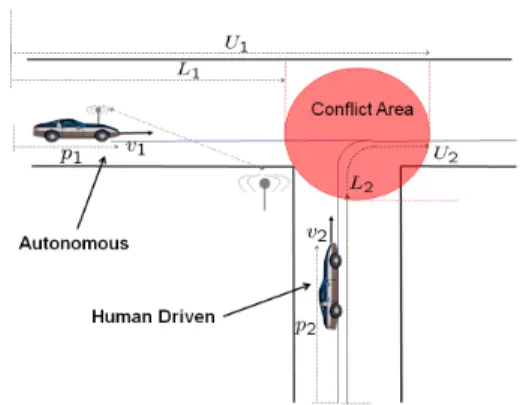
Fig. 1. Two-vehicle Conflict Scenario. Vehicle 1 (autonomous)
is equipped with a cooperative active safety system and commu-nicates with the infrastructure via wireless. Vehicle 2 (human-driven) is not equipped and does not communicate with the infrastructure. A collision occurs when more than one vehicle occupies the conflict area at one time.
Rch( ¯q), and by property (iii) of Proposition 2 from [20], it follows that ˆC¯q ⊇ Pre(¯q, ˆCRch( ¯q)). In turn we have that
ˆ
CRch( ¯q) ⊇ Pre(Rch(¯q), Bad) by Proposition 4 of [20] and
property (iii) of Proposition 2 from [20]. Hence, we have that ˆC¯q ⊇ Pre(¯q, Pre(Rch(¯q), Bad)), which by property (i)
of Proposition 2 from [20] leads to ˆC¯q⊇ Pre(Rch(¯q), Bad).
! This result shows that the mode-dependent capture set ˆ
C¯q can be computed by computing the Pre operator only
once as opposed to being determined through a (finite, by Theorem 2 and Proposition 4) iteration of Pre operator computations (as was performed in [20, 21]). To illustrate this point, consider as an example a tuple ( ˆR, ˆQ, Y) with
ˆ
Q = {ˆq1, ˆq2}, Y = {!, y}, ˆR(ˆq1, y) = ˆq2 and ˆR( ˆq2, y) = ˆq1
with ˆq1 ! ˆq2. Since there is a loop between ˆq1 and ˆq2
and the kernel set does not contain a maximal element, Theorem 2 of [20] cannot guarantee the termination of Algorithm 1. However, the results presented in this paper show that the desired capture set can be obtained by utilizing Lemma 1, that is, ˆCˆq1 =Pre(Rch( ˆq1), Bad) and
ˆ
Cˆq2 =Pre(Rch( ˆq2), Bad), in which Rch( ˆq2) = Rch( ˆq1) =
{ˆq1, ˆq2}. The computation of such a Pre can be efficiently
performed if the continuous dynamics for q ∈ ˆq1∪ ˆq2
has suitable order preserving properties [23]. We show an application example in the next section.
IV. Application scenario
Referring to Figure 1, vehicle 1 is autonomous and communicates with the infrastructure, while vehicle 2 is human-driven and does not communicate its intent to the infrastructure nor to the other vehicle. We assume that the infrastructure measures the position and speed of vehicle 2 through road-side sensors such as cameras and magnetic-induction loops and that it transmits this information to the on-board controller of vehicle 1. Vehicle 1 has to use this information to avoid a collision.We assume that the
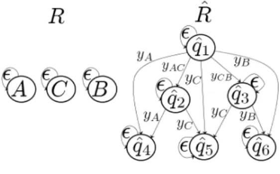
Fig. 2. Map R and map ˆR.
human driver decides to either accelerate (A), coast (C) or brake (B) the vehicle when he/she is near the intersec-tion. The intersection system is a hybrid automaton with uncontrolled mode transitions H, in which Q ={A, C, B};
X = R4 and x∈ X is such that x = (p
1, v1, p2, v2), where
pi is the longitudinal displacement along the path and vi
is the longitudinal speed of the ith vehicle, with i∈ {1, 2};
U = [uL, uH] ⊂ R represents the maximum braking and
throttle control input; D = [− ¯d, ¯d] ⊂ R; Σ = {!} as there is no transition allowed between the modes; R : Q× Σ → Q is the mode update map, and f : X× Q×U × D → X is the vector field, which is piecewise continuous and is given by f (x, q, u, d) = ( f1(p1, v1, u), f2(p2, v2, q, d)) in which f1(p1, v1, u) = v1 0 if (v1=vminand α1< 0) or (v1=vmaxand α1> 0) α1 otherwise , f2(p2, v2, q, d) = v2 0 if (v2=vminand α2 < 0) or (v1=vmaxand α2> 0) α2 otherwise , with α1=au + b− cv21; α2= βq+d; b < 0 represents the
static friction term; c > 0 with the cv2
1 term modeling
air drag (see [13, 22] for more details on the model);
q ∈ {A, C, B}; d ∈ [− ¯d, ¯d] and ¯d > 0. The value of βq
corresponds to the nominal dynamics of mode q and thus βA > 0, βC=0 and βB< 0. The disturbance d models the
error with respect to the nominal mode. There is a lower non-negative speed limit, vmin, implying that vehicles
can-not go in reverse and guaranteeing liveness of the system. Similarly there is an upper speed limit, denoted vmax. The
assumption that the driver cannot change his mind once he selects a mode is a fair assumption near an intersection. In [12], the authors study drivers who either accelerate or brake while approaching a traffic light. Driver behavior that allows switching from acceleration to coasting to braking is considered in [23]. Referring to Figure 1, the set of bad states for system H models collision configurations and it is given by Bad :={(p1, v1, p2, v2)∈ R4 | (p1, p2)∈
[L1, U1]× [L2, U2]}.
The system ˆH = ( ˆQ, X, U, D, Y, ˆInv, ˆR, f ), in which ˆQ =
{ˆq1, ˆq2, ˆq3, ˆq4, ˆq5, ˆq6} with ˆq1={A, C, B}, ˆq2={A, C}, ˆq3=
{C, B}, ˆq4 = {A}, ˆq5 = {C}, ˆq6 = {B}, and ˆq(0) = ˆq1, is
uniquely defined once the set Y and map ˆR are defined.
We define Y ={yAC, yCB, yA, yC, yB, !}. Let us consider the
following estimate ˆβ(t) = 1t5t−Tt ˙v2(τ)dτ, t ≥ T,1where
T > 0 is a time window ( ˆβ(t) is the average acceleration
over time window of length T ). If the mode is q, then we have that| ˆβ(t)−βq| ≤ ¯d. Thus, for t > T, define y(t) = yAif
|ˆβ(t)−βC| > ¯d and | ˆβ(t)−βB| > ¯d; y(t) = yCif| ˆβ(t)−βA| > ¯d
and| ˆβ(t) − βB| > ¯d; y(t) = yB if | ˆβ(t) − βA| > ¯d and | ˆβ(t) −
βC| > ¯d; y(t) = yAC if| ˆβ(t) − βC| ≤ ¯d, | ˆβ(t) − βA| ≤ ¯d and
|ˆβ(t) − βB| > ¯d; y(t) = yCB if| ˆβ(t) − βB| ≤ ¯d, | ˆβ(t) − βC| ≤ ¯d
and| ˆβ(t)−βA| > ¯d; and y(t) = ! otherwise. The resulting ˆR
is shown in Figure 2. For system ˆH, we have from Lemma
1 that ˆCˆqi = Pre( ˆqi, Bad) for i∈ {1, 2, 3, 4, 5, 6}. Since a
mode switch is not allowed, identifying the mode reduces the size of the capture set.
The sets Pre( ˆqi, Bad) can be easily calculated with a
linear complexity discrete time algorithm, as in the ith
mode the dynamics are given by the parallel composition of two order-preserving systems and Bad is an interval [11]. In particular, these sets are given as Pre( ˆq, Bad) = Pre( ˆq, Bad)L ∩ Pre(ˆq, Bad)H, in which Pre( ˆq, Bad)L =
{x ∈ X | ∃ t, d s.t. some φˆx(t, (x, ˆq), d, uL, !) ∈
Bad} and Pre( ˆq, Bad)H = {x ∈
X | ∃ t, d s.t. some φˆx(t, (x, ˆq), d, uH, !) ∈ Bad}
(see [7, 11] for more details on these computational techniques). The map ˆπ( ˆq, x) for every mode estimate ˆq is active only when x is on the boundary of ˆCˆq and in
such a case it makes the continuous state slide on the boundary of ˆCˆq [7, 11]. A feedback map ˆπ( ˆq, x), that
satisfies Theorem 1 is given by ˆπ( ˆq, x) :=
uL i f x∈ Pre(ˆq, Bad)H∧ x ∈ ∂Pre(ˆq, Bad)L
uH i f x∈ Pre(ˆq, Bad)L∧ x ∈ ∂Pre(ˆq, Bad)H
uL i f x∈ ∂Pre(ˆq, Bad)L∧ x ∈ ∂Pre(ˆq, Bad)H
∗ otherwise.
Simulation results are shown in Figure 3. V. Conclusion
In this paper, we considered the problem of safety control of hidden mode hybrid systems. In particular, we solve the problem by utilizing an existing approach from [20, 21] to construct a new hybrid automaton (an estimator) whose discrete state is an estimate of the hidden mode. The main contribution of this work is in showing that the algorithm that computes the capture set is guaranteed to terminate under substantially less restrictive conditions than those considered in [20, 21]. Moreover, we provide a simple formula for the computation of the capture set. Independently of the number of discrete states in the estimator, the capture set for each discrete state is efficiently calculable for systems whose continuous
1Note that in practice, we will not require measurement of acceleration
as we will consider discrete time models where derivative is replaced by time anticipation.
0 200 400 600 0 100 200 300 400 500 600 x 1 x3 (a) 00 200 400 600 100 200 300 400 500 600 x 1 x3 (b) 0 200 400 600 0 100 200 300 400 500 600 x1 x3 (c) 00 200 400 600 100 200 300 400 500 600 x1 x3 (d) 00 200 400 600 100 200 300 400 500 600 x1 x3 (e)
Fig. 3. In each of the plots (a)–(e), the red box represents
[L1, U1]×[L2, U2]. We plot the slice of ˆCˆqin the (x1, x3) position
plane corresponding to the current speed (x2, x4). In the (x1, x3)
plane and for the current speed values (x2, x4), the black solid
lines delimit the set Pre( ˆq, Bad)H, the green dashed lines delimit
the set Pre( ˆq, Bad)Land the intersection of these two sets is the
current mode dependent capture set ˆCˆq. The red circle denotes
the current position x1, x3, while the blue trace represents the
projection in the position plane of the continuous trajectory of H. Plot (a) shows the initial configuration in the position plane. Here, the current mode estimate is ˆq ={A, C, B}. Plot (b) shows the mode estimate switching to ˆq ={C, B} and the corresponding capture set shrinking. Plot (c) shows the time at which the mode estimate becomes ˆq ={B}, so that the current mode is locked and the capture set shrinks further. Plot (d) shows when the continuous state hits the boundary of the current mode-dependent capture set thus resulting in the application of a safe control. dynamics have suitable order-preserving properties [23]. We introduce an example of a semi-autonomous cooper-ative active safety system that belongs to this class and present simulation results for collision avoidance between a human-driven and an autonomous vehicle merging at an intersection. In future work, we intend to consider situations with more than two vehicles merging on an intersection, in which some of the vehicles are human-driven and some are autonomous. The approach presented in this paper cannot be directly extended to the multiple vehicle scenario due to the bad set not being convex. Alternative approaches are being investigated, including discrete abstraction techniques exploiting the fact that the vehicles dynamics are differentially flat and order preserving [4].
References
[1] M. Althoff. Reachability Analysis and its Application to the
Safety Assessment of Autonomous Cars. PhD thesis, Technische
Universitat Munchen, 2010.
[2] J. Aubin. Viability Theory. Birkh¨auser, 1991.
[3] A. Balluchi, L. Benvenuti, M. D. Di Benedetto S, and A. L. Sangiovanni-vincentelli. Design of observers for hybrid systems. In In Hybrid Systems: Computation and Control, volume 2289 of
LNCS, pages 76–89. Springer-Verlag, 2002.
[4] A. Colombo and D. Del Vecchio. Supervisory control of differen-tially flat systems based on abstraction. In Conf. on Decision and
Control, 2011. to appear.
[5] D. Del Vecchio. A partial order approach to discrete dynamic
feedback in a class of hybrid systems. In Hybrid Systems:
Computation and Control, Lecture Notes in Computer Science, vol.
4416, A. Bemporad, A. Bicchi, and G. Buttazzo (Eds.), Springer Verlag, pages 159–173, Pisa, Italy, 2007.
[6] D. Del Vecchio. Observer-based control of block triangular discrete time hybrid automata on a partial order. International Journal of
Robust and Nonlinear Control, 19(14):1581–1602, 2009.
[7] D. Del Vecchio, M. Malisoff, and R. Verma. A separation principle for a class of hybrid automata on a partial order. In American
Control Conference, pages 3638–3643, 2009.
[8] D. Del Vecchio, R. M. Murray, and E. Klavins. Discrete state estimators for systems on a lattice. Automatica, 42(2):271–285, 2006.
[9] D. Del Vecchio, R. M. Murray, and P. Perona. Decomposition of human motion into dynamics-based primitives with application to drawing tasks. Automatica, 39(12):2085–2098, 2003.
[10] D. Caveney H. Kowshik and P. R. Kumar. Provable systemwide safety in intelligent intersections. IEEE Transactions on Automatic
Control, 60(3):804–818, March 2007.
[11] M. Hafner and D. Del Vecchio. Computation of safety control for uncertain piecewise continuous systems on a partial order. In
Conference on Decision and Control, pages 1671 –1677, 2009.
[12] J. K. Hedrick, Y. Chen, and S. Mahal. Optimized vehicle con-trol/communication interaction in an automated highway system.
Virginia Tech Transportation Institute: Report No. VPI-2006-06.,
2008.
[13] Uwe Kiencke and Lars Nielsen. Automotive Control Systems, For
Engine, Driveline, and Vehicle. Springer Verlag, 2nd edition, 2005.
[14] A. B. Kurzhanski and P. Varaiya. Ellipsoidal techniques for
hybrid dynamics: the reachability problem. In New Directions
and Applications in Control Theory, Lecture Notes in Control and
Information Sciences, vol 321, W.P. Dayawansa, A. Lindquist, and Y. Zhou (Eds.), pages 193–205, 2005.
[15] C. Le Guernic. Reachability Analysis of Hybrid Systems with
Lin-ear Continuous Dynamics. PhD thesis, Univerite Joseph Fourier,
2009.
[16] J. Lygeros, C. J. Tomlin, and S. Sastry. Controllers for reachability
specifications for hybrid systems. Automatica, 35(3):349–370,
1999.
[17] Meeko Oishi, Ian Mitchell, Alexandre Bayen, and Claire Tomlin. Invariance-preserving abstractions of hybrid systems: Application to user interface design. IEEE Transactions on Control Systems
Technology, 16(2):229–244, March 2008.
[18] O. Shakernia, G. J. Pappas, and Shankar Sastry. Semi-decidable
synthesis for triangular hybrid systems. In Hybrid Systems:
Computation and Control, Lecture Notes in Computer Science, vol.
2034, M. D. Di Benedetto and A. Sangiovanni-Vincentelli (Eds.), Springer Verlag, 2001.
[19] C. J. Tomlin, I. Mitchell, A. M. Bayen, and M. Oishi. Computa-tional techniques for the verification of hybrid systems.
Proceed-ings of the IEEE, 91(7):986–1001, 2003.
[20] R. Verma and D. Del Vecchio. Continuous control of hybrid
automata with imperfect mode information assuming separation between state estimation and control. In Conference on Decision
and Control, pages 3175 –3181, 2009.
[21] R. Verma and D. Del Vecchio. Control of hybrid automata with hidden modes: translation to a perfect state information problem. In Conference on Decision and Control, pages 5768 –5774, 2010.
[22] R. Verma, D. Del Vecchio, and H. Fathy. Development of a
scaled vehicle with longitudinal dynamics of a HMMWV for an ITS testbed. IEEE/ASME Transactions on Mechatronics, 13:46–57, 2008.
[23] R. Verma and D. Del Vecchio. Safety control of hidden mode hybrid systems. IEEE Transactions on Automatic Control, 2011. to appear.
[24] M. De Wulf, L. Doyen, and J.-F. Raskin. A lattice theory
for solving games of imperfect information. Hybrid Systems:
Computation and Control, Lecture Notes in Computer Science, vol.
3927, J. Hespanha and A. Tiwari (Eds.), Springer-Verlag, pages 153–168, 2006.
![Fig. 3. In each of the plots (a)–(e), the red box represents [L 1 , U 1 ] × [L 2 , U 2 ]](https://thumb-eu.123doks.com/thumbv2/123doknet/14478725.523634/8.918.135.442.109.303/fig-plots-red-box-represents-l-u-l.webp)
