HAL Id: hal-00298942
https://hal.archives-ouvertes.fr/hal-00298942
Submitted on 9 Apr 2008HAL is a multi-disciplinary open access
archive for the deposit and dissemination of sci-entific research documents, whether they are pub-lished or not. The documents may come from teaching and research institutions in France or abroad, or from public or private research centers.
L’archive ouverte pluridisciplinaire HAL, est destinée au dépôt et à la diffusion de documents scientifiques de niveau recherche, publiés ou non, émanant des établissements d’enseignement et de recherche français ou étrangers, des laboratoires publics ou privés.
The influence of heterogeneous groundwater discharge
on the timescales of contaminant mass flux from
streambed sediments ? field evidence and long-term
predictions
C. Schmidt, E. Kalbus, M. Martienssen, M. Schirmer
To cite this version:
C. Schmidt, E. Kalbus, M. Martienssen, M. Schirmer. The influence of heterogeneous groundwater discharge on the timescales of contaminant mass flux from streambed sediments ? field evidence and long-term predictions. Hydrology and Earth System Sciences Discussions, European Geosciences Union, 2008, 5 (2), pp.971-1001. �hal-00298942�
HESSD
5, 971–1001, 2008 Contaminant mass fluxes from streambed sediments C. Schmidt et al. Title Page Abstract Introduction Conclusions References Tables Figures ◭ ◮ ◭ ◮ Back Close Full Screen / EscPrinter-friendly Version Interactive Discussion Hydrol. Earth Syst. Sci. Discuss., 5, 971–1001, 2008
www.hydrol-earth-syst-sci-discuss.net/5/971/2008/ © Author(s) 2008. This work is distributed under the Creative Commons Attribution 3.0 License.
Hydrology and Earth System Sciences Discussions
Papers published in Hydrology and Earth System Sciences Discussions are under open-access review for the journal Hydrology and Earth System Sciences
The influence of heterogeneous
groundwater discharge on the timescales
of contaminant mass flux from streambed
sediments – field evidence and long-term
predictions
∗
C. Schmidt1, E. Kalbus1, M. Martienssen2, and M. Schirmer3 1
UFZ, Helmholtz Centre for Environmental Research, Dept. of Hydrogeology, Leipzig, Germany
2
UFZ, Helmholtz Centre for Environmental Research, Dept. of Hydrogeology, Halle, Germany 3
Swiss Federal Institute of Aquatic Science and Technology, EAWAG, Dept. of Water Resources and Drinking Water, D ¨ubendorf, Switzerland
Received: 11 March 2008 – Accepted: 17 March 2008 – Published: 9 April 2008 Correspondence to: C. Schmidt (christian.schmidt@ufz.de)
Published by Copernicus Publications on behalf of the European Geosciences Union.
HESSD
5, 971–1001, 2008 Contaminant mass fluxes from streambed sediments C. Schmidt et al. Title Page Abstract Introduction Conclusions References Tables Figures ◭ ◮ ◭ ◮ Back Close Full Screen / EscPrinter-friendly Version Interactive Discussion
Abstract
Streambed sediments can act as long-term storage zones for organic contaminants originating from the stream water. Until the early 1990s, the small man-made stream, subject of our study, in the industrial area of Bitterfeld (Germany), was used for waste water discharge from the chemical industry nearby. The occurrence of contaminants in
5
the streambed is resulting from aqueous-phase transport and particle facilitated depo-sition. Groundwater discharge through the streambed can otherwise induce a remobi-lization and an advective contaminant flux so that contaminants are released back from the streambed to the stream water. We investigated the long-term mass flow rates of chlorinated benzenes (MCB, DCBs) from the streambed to the overlying stream water
10
driven by advection of groundwater. The spatial patterns and magnitudes of groundwa-ter discharge were examined along a reach of 220 m length. At 140 locations ground-water discharge was quantified using streambed temperatures and ranged from 11.0 to 455.0 Lm−2d−1. According to locations with high and low groundwater discharge,
time-integrating passive samplers were used to monitor current contaminant
concen-15
trations in the streambed. Streambed contaminant concentrations at high groundwater discharge locations were found to be lower than at low discharge locations. Based on data from batch experiments and field observations we parameterized and run multiple one-dimensional advective transport models for the observed range of groundwater discharge magnitudes to simulate the timescales of contaminant release and their
de-20
pendence on the magnitude of groundwater discharge. The results of the long-term predictive modeling revealed that the time required to reduce the concentrations and the resulting mass fluxes to the water to 10% of the initial values will be in the scale of decades for high-discharge locations and centuries for low-discharge locations, re-spectively.
25
HESSD
5, 971–1001, 2008 Contaminant mass fluxes from streambed sediments C. Schmidt et al. Title Page Abstract Introduction Conclusions References Tables Figures ◭ ◮ ◭ ◮ Back Close Full Screen / EscPrinter-friendly Version Interactive Discussion
1 Introduction
Streambed sediments often act as long-term storage zones for organic contaminants and metals. The occurrence of contaminants in the streambed is a result of aqueous-phase transport, particle facilitated deposition and sorption to sediments. Contami-nants may enter the streambed either by infiltration of stream water into the sediments
5
(e.g., Zaramella, 2006; W ¨ormann, 1998) or by discharging groundwater (e.g., Conant et al., 2004). When the streambed sediments are permeable, hyporheic exchange and groundwater discharge drive advective transport with the streambed. Advection con-trols or is coupled to biogeochemical processes (Cardenas and Wilson, 2007; Jones and Mullholland, 2000).
10
In temperate climates, groundwater typically discharges into surface water bodies such as streams and rivers. When contaminated groundwater discharges to a stream, the contaminant plume might get substantially modified in its concentration distribu-tion and composidistribu-tion during the passage through the streambed and the near-stream zone (Conant et al., 2004). However, the discharge of contaminated groundwater to a
15
stream, either as a diffuse contamination or as a distinct contaminant plume, may be associated with significant mass fluxes of contaminants to the surface water system (Kalbus et al., 2007; Chapman et al., 2007). On the other hand, the discharge of un-contaminated groundwater may induce the release and transport of contaminants from streambed sediments to the surface water. In this case, the advection of groundwater
20
and the apparent mass transfer from the sediment may be the governing processes that control mass fluxes (Lick, 2006; Schmidt et al., 2008).
In the literature, a few field studies can be found addressing contaminant fluxes to surface waters associated with groundwater discharge. The majority of the studies focused on characterizing the spatial distribution of contaminants in the streambed
25
and the adjacent aquifer when a plume discharges to the surface water (Conant et al., 2004; Lorah and Olsen, 1999; Westbrook et al., 2005) or on mapped plan-view distributions of contaminants in the streambed (Vroblesky, 1991). Site assessment
HESSD
5, 971–1001, 2008 Contaminant mass fluxes from streambed sediments C. Schmidt et al. Title Page Abstract Introduction Conclusions References Tables Figures ◭ ◮ ◭ ◮ Back Close Full Screen / EscPrinter-friendly Version Interactive Discussion and remediation design may benefit from determining contaminant mass flow rates as
alternative criterion instead of maximum concentration levels. Recently, approaches were published to quantify contaminant mass fluxes and contaminant mass flow rates to streams (Chapman et al., 2007; Kalbus et al., 2007; Schmidt et al., 2008). Schmidt et al. (2008) showed that contaminated streambed sediments can substantially contribute
5
to contaminant mass flow into the stream water.
Even after the source areas at contaminated sites have been cleaned up, the con-taminants stored in the streambed sediments, originating either from the surface water or from groundwater plumes, may be released from the sediments back to the stream and may represent a dominant, long-term contamination source for downstream
ar-10
eas. Processes that contribute to the sediment-water transfer of contaminants include molecular diffusion, bioturbation, and pore-water advection due to groundwater dis-charge (Erickson et al., 2005). These processes are usually lumped together and modelled as diffusive flux by means of a mass transfer approximation (Lick, 2006). In this study, however, we highlight the potential influence of groundwater discharge on
15
the mass flow rates from the streambed to the overlying stream water. In particular, the study focuses on the influence of spatial patterns of groundwater discharge on contaminant mass flow rates along a 220 m long reach. We hypothesize that spatial heterogeneities of groundwater discharge influence the timescales of contaminant re-lease from the streambed to the stream. The contaminant mass flux entering a stream
20
with the discharging groundwater depends on the concentration of contaminants in the groundwater and the water flux across the streambed. The total contaminant mass flux entering the stream will decay with time because contaminants will be successively removed, controlled by the desorption behaviour of the specific compound.
At a small stream in Germany, we selected different locations with respect to the
25
magnitude of groundwater flux through the streambed. At these locations we installed passive samplers in the streambed to characterize the current contaminant distribution. Batch experiments were conducted to elucidate the desorption behaviour of the tar-get compounds monochlorobenzene (MCB) and the isomers of dichlorobenzene
HESSD
5, 971–1001, 2008 Contaminant mass fluxes from streambed sediments C. Schmidt et al. Title Page Abstract Introduction Conclusions References Tables Figures ◭ ◮ ◭ ◮ Back Close Full Screen / EscPrinter-friendly Version Interactive Discussion DCB, 1,3-DCB, 1,4-DCB) as input data for a streambed transport model. We applied
a numerical one-dimensional advective transport model to predict the timescales of contaminant release and their dependence on the magnitude and spatial patterns of groundwater discharge.
2 Study site
5
The study was carried out in the industrial area of Bitterfeld/Wolfen, about 130 km south of Berlin, Germany (Fig. 1). The region is one of the oldest centres of chemical indus-try in Germany (Heidrich et al., 2004a, b). One century of chemical production has resulted in a regional groundwater contamination with an estimated extent of 25 km2 (Weiß et al., 2001). The main contaminants are volatile halogenated hydrocarbons,
10
monoaromatic hydrocarbons such as BTEX or chlorinated benzenes and phenols, hex-achlorocyclohexanes (HCH), polychlorinated biphenyls, dioxins, and a variety of other substances. Soils and floodplain sediments downstream of the site show increased levels of persistent organic contaminants such asβ-HCH, a waste product of former
lindane (γ-HCH) production (Barth et al., 2007).
15
The investigations were conducted along a 220 m long reach of the Schachtgraben. The stream is part of the Mulde River system which is a tributary to the Elbe River. The Schachtgraben was man-made and had originally been constructed for mine wa-ter discharge from open-cast lignite mines. Lawa-ter, it was also used for waste wawa-ter discharge from the chemical industry for a period of three decades until 1990. In the
20
early 1990s, monitoring programmes revealed a rapid decline of organic contaminants between 1990 and 1992 in the streams and rivers downstream of the study site, in particular in the Mulde River (LSA, 1993). In 1993, chlorinated benzenes were the substances with highest individual concentrations observed in the Mulde River with, for example, MCB concentrations up to 31µg L−1 (LSA, 1993). This value is quite
im-25
pressive when considering the mass flow rate since the average stream flow rate in the Mulde River is approximately 60 m3s−1 (Schachtgraben: 0.2 m3s−1, Kalbus et al.,
HESSD
5, 971–1001, 2008 Contaminant mass fluxes from streambed sediments C. Schmidt et al. Title Page Abstract Introduction Conclusions References Tables Figures ◭ ◮ ◭ ◮ Back Close Full Screen / EscPrinter-friendly Version Interactive Discussion 2007). Unfortunately, no monitoring data from the Schachtgraben itself is available for
this time. A recent report of a monthly monitoring programme in the Mulde River re-vealed a maximum concentration of MCB of 0.06µ g L−1 (LSA, 2005). In comparison,
during a five-day pumping test in October 2005 of Kalbus et al. (2007), the average concentration of MCB in the Schachtgraben was 24.7µg L−1.
5
The streambed of the Schachtgraben consists of a 0.6 m thick layer of crushed rock. The pore space of the crushed rock layer is filled with autochtone, sandy, fluviatile material. The stream is about 3 m wide and has an average water depth of 0.6 m. It partially penetrates a Quaternary alluvial Aquifer. The water table in the aquifer is generally higher than the water level in the stream. Hence, the Schachtgraben can be
10
classified as a gaining stream. To characterize the interaction between the groundwa-ter and the stream, Schmidt et al. (2006) recorded 140 streambed temperature profiles in the summer of 2005. The water fluxes through the streambed can be estimated based on observed streambed temperatures (Conant, 2004; Schmidt et al., 2007). At the study site, the water fluxes ranged from 455 Lm−2d−1 of groundwater discharge
15
to 10 Lm−2d−1 of stream water entering the streambed (Schmidt et al., 2006). The
dominant contaminants in the Quaternary aquifer are chlorinated benzenes. The main contamination source is believed to be about 3.5 km south of the study site. Preliminary investigations showed that the contamination level of pore water in the streambed sed-iments is significantly higher than in the alluvial aquifer (Schmidt et al., 2008; Kalbus et
20
al., 2007). After the close-down of main parts of the chemical industry and the imple-mentation of new environmental regulations and waste water treatment facilities, the contaminant release from streambed sediments and the discharge of contaminated groundwater became the dominant contamination source for the streams and rivers at the site, which is persisting until today.
25
HESSD
5, 971–1001, 2008 Contaminant mass fluxes from streambed sediments C. Schmidt et al. Title Page Abstract Introduction Conclusions References Tables Figures ◭ ◮ ◭ ◮ Back Close Full Screen / EscPrinter-friendly Version Interactive Discussion
3 Methods
3.1 Passive sampling
Snapshot sampling of contaminant concentrations in the streambed and contaminant mass flux calculations already identified the streambed as a current source of con-taminants (Schmidt et al., 2008). However, to gain further insight into the transport
5
processes to the streambed, it is expedient to obtain depth-orientated profiles of con-taminant concentrations within the upper streambed layer. Because the streambed of the Schachtgraben is constructed of crushed rock, it turned out to be difficult to take sediment cores or to install streambed piezometers to conduct depth-oriented snapshot sampling of the pore water. Hence, to achieve robust estimates of contaminant
con-10
centrations with fine vertical spatial resolution, time-integrating passive samplers were deployed in the streambed. These devices can be placed directly in the streambed sed-iments at well-defined depths and presumed to be capable to capture representative aqueous concentrations. Additionally, possible short-term variations in aqueous con-centrations are averaged by time-integrating samplers. However, if frequent changes
15
in the flow direction occur the averaging might be problematic for the calculation of mass fluxes (Kalbus et al., 2006). But hydraulic head observations suggest that the Schachtgraben is constantly a gaining stream.
The passive sampling system used in this study (ceramic dosimeter, Bopp et al., 2005) consists of 4.5 cm long ceramic tubes filled with an adsorbent material. To
pre-20
vent the dosimeter from damages, a steel casing was used (see Fig. 1 in Bopp et al., 2005), which increased the entire length of the passive sampling system to 5.0 cm. In order to obtain depth-orientated estimates of contaminant concentrations, we de-ployed the dosimeters at four different depths at each sampling location (0.10–0.15, 0.20–0.25, 0.30–0.35 and 0.40–0.45 m below the streambed surface) in the streambed
25
sediments. The sampling locations were chosen with respect to the groundwater dis-charge regime as identified by Schmidt et al. (2006) in a previous study. One array of dosimeters (array 1) was deployed at a low-discharge zone with a groundwater flux
HESSD
5, 971–1001, 2008 Contaminant mass fluxes from streambed sediments C. Schmidt et al. Title Page Abstract Introduction Conclusions References Tables Figures ◭ ◮ ◭ ◮ Back Close Full Screen / EscPrinter-friendly Version Interactive Discussion of 10 Lm−2d−1, arrays 2 and 3 were placed at high-discharge zones with fluxes of
300–400 Lm−2d−1. Additionally, two dosimeters were placed in groundwater
monitor-ing wells and two were deployed in the surface water (Fig. 1). The ceramic dosimeters stayed in the streambed, surface water and groundwater from June–September 2006. Contaminants are diffusing across the ceramic membrane and are adsorbed over
5
the entire sampling period at the adsorbent material. The average contaminant con-centration in the water can be obtained from the adsorbed contaminant mass and the duration of exposure (Martin et al., 2003; Bopp et al., 2005). The parameters required to derive the average concentration from the adsorbed mass are given in Table 1. For sample extraction from the adsorbent material within the ceramic dosimeters a
modi-10
fication of the method described by Bopp et al. (2005) was used. Prior to extraction, the metal cage of the ceramic dosimeter was opened and the caps were removed. In the first step, the adsorbent material was extracted two times with 5 mL of acetone and 5 min contact time. To obtain a duplicate sample, the procedure was repeated.
3.2 Batch experiments
15
Batch experiments were conducted with the streambed sediments to study the desorp-tion behaviour of the target compounds and obtain input parameters for the streambed transport model. Since the crushed rock in the streambed precluded successful sed-iment coring, pooled sedsed-iment samples were taken that integrated the upper 0.5 m of the streambed.
20
For the determination of the sediment-water partitioning coefficient a volume of 50 mL of water was added to different masses of sediments (4.2, 7.5, 14.6, 29.4, 60.9, 118.0, 218.9, 369.9 g (dry)) in 250 mL glass bottles. The bottles were placed on a mechanical tumbler and were incubated for 48 h. After that incubation period, the su-pernatants were removed and analyzed for contaminant concentrations by
Headspace-25
GC/MS (Varian GC/MS, Type CP 3800 MS1200, Column 60 m Zebron ZB1, Injection 1 ml). To determine the initial sediment contaminant concentrations were 10.1 g of fresh
HESSD
5, 971–1001, 2008 Contaminant mass fluxes from streambed sediments C. Schmidt et al. Title Page Abstract Introduction Conclusions References Tables Figures ◭ ◮ ◭ ◮ Back Close Full Screen / EscPrinter-friendly Version Interactive Discussion sediment were extracted with 20 ml Acetone and analysed in the GC.
The sediment-water partitioning coefficient (Kd) was calculated for each
sediment-water ratio. For the subsequent calculations the averageKd value was applied. The contaminant release andKd were determined based on the liquid phase concentrations
by assuming that changes in the liquid-phase concentrations are equal to changes in
5
sediment contaminant concentrations.
Additionally, two batch desorption experiments were carried out parallel in 10 bottles. In the first experiment, 100 g sediment and 20 mL of water were filled into each bottle. The concentration of the target compound was measured in the water using the same analytic procedure as for the determination of the partition coefficient. The compound
10
concentrations were determined after 2, 4, 8, 16, 24, 48, 72, 96, and 168 h. In a second experiment, 100 g sediment and 30 mL of water were filled into each bottle and the compound concentrations were measured after 0.5, 1, 2, 3, 4, 5, 6, and 24 h to experimentally underpin the quasi-instantaneous equilibrium assumption.
3.3 Modelling approach
15
The underlying idea of this study is to show that spatially heterogeneous groundwater discharge affects the release and the resulting mass flow rates of contaminants from the streambed to the stream along a reach. For this purpose, we selected a very simple modelling approach that accounts for groundwater advection but simplifies the desorptive mass transfer to a linear equilibrium process. Moreover, it is assumed that
20
flow and transport through the streambed are vertical and steady. We further assume that advection is the governing process along the short flow domain of 1 m in length and hence, we do not consider dispersion. The governing equation for one-dimensional advective transport is given with:
∂Cw ∂t = − qz/ne R ∂Cw ∂z (1) 25
HESSD
5, 971–1001, 2008 Contaminant mass fluxes from streambed sediments C. Schmidt et al. Title Page Abstract Introduction Conclusions References Tables Figures ◭ ◮ ◭ ◮ Back Close Full Screen / EscPrinter-friendly Version Interactive Discussion whereCw is the concentration of the contaminant in the pore water,qz is the vertical
Darcy flux (positive upward),R is the retardation factor, z is the vertical spatial
coordi-nate,t is the time, and ne is the effective porosity. Batch experiments indicated that it is reasonable to apply a simple linear isotherm. The retardation factorR is then given
with:
5
R = 1 +nρ
e
Kd (2)
whereρ is the bulk density of the sediment and Kd is the sediment-water partitioning coefficient.
The sediment properties are assumed to be homogeneous at all locations with a homogeneous initial contaminant load of the sediment. The only parameter variable in
10
space isqz.
Simulations were run until the contaminant load of the sediment (Cs) has decreased
by 90% from its initial value at the outflow (the sediment water interface) of the domain. To predict the timescales of contaminant release it is not required to know the absolute concentrations since the timescales are only depending onqz andKd.
15
We used an explicit finite difference approximation to calculate the removal of each target compound from the sediment layer with equation 1. The model domain was set to a thickness of 1 m with a space increment of 0.04 m. The time step was set to 0.5 days to comply with the Courant criteria for numerical stability. The water fluxes (qz) for each observation point were taken from the results of Schmidt et al. (2006).
20
The contaminant mass flux can be calculated for each observation point (x, y) for
time t from qz(x, y)×Cout(t). The total contaminant mass flow rate through a given
area of the streambedS as a function of time can be calculated using:
MS(t) =
Z
S
qz(x, y)Cout(t)d S (3)
For the evaluation of timescales and the influence of the heterogeneity of groundwater
25
discharge, contaminant mass flow rates were normalized byMS(t)/MSi whereMSi is
HESSD
5, 971–1001, 2008 Contaminant mass fluxes from streambed sediments C. Schmidt et al. Title Page Abstract Introduction Conclusions References Tables Figures ◭ ◮ ◭ ◮ Back Close Full Screen / EscPrinter-friendly Version Interactive Discussion the calculated total mass flow rate att0.
4 Results and discussion
4.1 Current contaminant concentrations
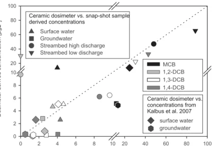
Aqueous concentrations from the ceramic dosimeters versus aqueous concentrations from a snap-shot sampling programme parallel to the passive sampling are displayed
5
in Fig. 3. In addition, the aqueous concentrations in the groundwater and surface water obtained during an integral pumping test (IPT) at the study site by Kalbus et al. (2007) are plotted versus the dosimeter-derived concentrations. Overall, the concentrations derived from the ceramic dosimeters matched well the averaged concentrations from the snap-shot sampling. A slight tendency to underestimate the snap-shot sampling
10
results can be seen in Fig. 3. It seems that the dosimeters underestimate in partic-ular the concentrations in the groundwater, when compared with both the snap-shot sampling results and the IPT results. The scatter between dosimeter-derived aque-ous concentrations and snap-shot sampling-derived aqueaque-ous concentrations does not follow a substance-specific or sampling location-specific pattern. One significant
devi-15
ation is that no 1,2-DCB was detected in the snap-shot samples of the streambed but was found in the dosimeters. This is supposedly a random error because the results from groundwater and surface water matched reasonably. For the further discussion we consider the concentrations obtained from the dosimeters as representative.
The results show that concentrations in the interstitial pore water in the streambed
20
sediments were approximately one order of magnitude higher than in the groundwater and the surface water. Significant differences occur between zones of high and low groundwater discharge.
HESSD
5, 971–1001, 2008 Contaminant mass fluxes from streambed sediments C. Schmidt et al. Title Page Abstract Introduction Conclusions References Tables Figures ◭ ◮ ◭ ◮ Back Close Full Screen / EscPrinter-friendly Version Interactive Discussion 4.1.1 Contaminant concentrations in surface water and groundwater
Passive samplers deployed in the stream upstream and downstream of the investi-gated reach revealed comparable concentrations, which were generally (except for 1,4-DCB) slightly higher though at the upstream position closer to the chemical plant, where the source zone of the contaminants is located. At the upstream sampling
lo-5
cation the concentrations in the stream water were 14.1µg L−1 (MCB) and 0.8, 5.0,
2.6µg L−1 (1,2-DCB, 1,3-DCB, 1,4-DCB) and at the downstream location 13.8µg L−1
(MCB) and 0.9, 4.5, 2.8µg L−1 (1,2-DCB, 1,3-DCB, 1,4-DCB). Obviously, the inputs
from the streambed did not result in an increasing concentration in the surface water along the study reach of 220 m in length.
10
In two groundwater monitoring wells adjacent to the stream (Fig. 1) the monitored concentrations were characteristic for the diffuse background contamination present at the site with average values of 5.1µg L−1 (MCB) and 0.1, 0.2, 0.3µg L−1 (1,2-DCB,
1,3-DCB, 1,4-DCB). In one of the monitoring wells no DCB was observed (Fig. 4). A five-day IPT at four groundwater monitoring wells (in two of which dosimeters were
15
deployed) revealed average concentrations of 12.6µg L−1 MCB and 3.2µg L−1 DCB
(sum of isomers) (Kalbus et al., 2007). Average concentrations in the single wells ranged from 9.6 to 18.2µg L−1MCB and from 2.6 to 4.0µg L−1DCB (sum of isomers).
Hence, the background contamination of the groundwater can be assumed to be in the range of 5–20µg L−1 MCB and 2.5–4µg L−1 for the sum of isomers of DCB,
re-20
spectively. The inputs originating from the streambed are not necessarily reflected in the contaminant concentrations of the surface water because dilution and volatilization might significantly reduce the concentrations (Conant et al., 2004).
4.1.2 Aqueous concentrations in the streambed
In the streambed, the aqueous concentrations differed between zones of high and low
25
groundwater discharge as well as vertically at each passive sampler array. The highest concentrations were observed at the low-discharge zone (array 1), the lowest at one of
HESSD
5, 971–1001, 2008 Contaminant mass fluxes from streambed sediments C. Schmidt et al. Title Page Abstract Introduction Conclusions References Tables Figures ◭ ◮ ◭ ◮ Back Close Full Screen / EscPrinter-friendly Version Interactive Discussion the high-discharge zones (array 3). Average concentrations at the low-discharge zone
were 65.5µg L−1MCB, 6.5µg L−11,2-DCB, 22.4µg L−11,3-DCB and 32.9µg L−1
1,4-DCB. The two high-discharge zones, although spatially separated only by two metres, differed significantly in their average concentrations. At one zone (array 2) the aver-age concentration of MCB (65.6µg L−1) was similar to that at the low-discharge zone
5
(array 1). Conversely, the average concentrations of the DCB isomers (1.3µg L−1
1,2-DCB, 8.5µg L−1 1,3-DCB and 8.3µg L−1 1,4-DCB) at array 2 were within the order of
magnitude of the DCB concentrations at array 3 (0.7µg L−1 1,2-DCB, 4.4µg L−1
1,3-DCB and 4.1µg L−11,4-DCB). Overall, the aqueous contaminant concentrations in the
streambed were lower at zones of high groundwater discharge than at zones of low
10
groundwater discharge.
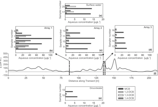
Focusing on the vertical distribution of contaminants in the streambed, Fig. 4 illus-trates that the lowest aqueous concentrations of all substances in the streambed were observed in the shallow dosimeters (no. 8, 12, 16) installed between 0.10–0.15 m be-low the streambed surface. In the arrays 1 and 2, the highest concentrations were
15
present at the subsequent depth of 0.20–0.25 m. Then, with increasing depth the concentrations decreased in the two arrays. Array 3 did not show this vertical pat-tern. Here, the concentrations of MCB increased from 33.6 to 24.6µg L−1 from the
top to the bottom of the streambed, while concentrations of DCB were virtually inde-pendent from the sampling depth (Fig. 4). The low aqueous concentrations at the
20
top of the streambed are likely a result of non-vertical hyporheic exchange between the streambed and the stream water. For greater depths, water flow and contaminant transport in the streambed is assumed to be essentially vertical towards the surface water. Schmidt et al. (2006) provide evidence to this assumption because their one-dimensional vertical water flow and heat advection model matches well the observed
25
temperature profiles.
The contamination of the streambed originates from the stream water which was highly contaminated during a period of approximately 25 years of intense waste water discharge from the chemical industry. The upper 0.6 m of the streambed consist of
HESSD
5, 971–1001, 2008 Contaminant mass fluxes from streambed sediments C. Schmidt et al. Title Page Abstract Introduction Conclusions References Tables Figures ◭ ◮ ◭ ◮ Back Close Full Screen / EscPrinter-friendly Version Interactive Discussion crushed rock. Deposition of fine, fluvially transported sediments in the pores of the
crushed rock layer was probably one main transport pathway of organic contaminants into the streambed, besides diffusion and hyporheic exchange. We therefore conclude that initially the upper 0.6 m of the streambed were nearly homogeneously contami-nated without any vertical gradients.
5
When the contamination level in the stream rapidly decreased after the close-down of main parts of the chemical industry in the early 1990s, the contaminant input to the streambed has presumably ceased. The relatively clean groundwater flowing into the contaminated sediment layer could then have induced the removal of contaminants starting at the bottom of the streambed. We interpret the observed decrease of the
10
aqueous concentrations with increasing depth as a result of this desorptive process. With time, the desorption front moves successively towards the top of the streambed. More than 15 years after the close-down of the chemical industry, the current vertical distribution of aqueous contaminant concentrations in the streambed indicates that the contaminant removal is still in progress.
15
4.2 Results of batch desorption experiments
The results of the desorption kinetic experiments for the target compounds are shown in Fig. 5. Each data point represents the remaining solid-phase fraction after a given time. The batch desorption experiment lasted 7 days. In general, only a very small fraction of the initial solid-phase contaminant load desorbed. The highest extent of
20
desorption was found for MCB. All isomers of DCB were characterized by a similar desorption behaviour showing no increase of the desorbed fraction with time (Fig. 5). In the first experiment, aqueous-phase concentrations were sampled after two hours (Fig. 5). In order to observe temporal desorption patterns, a second experiment was conducted where the first sample was taken after 30 min (Fig. 5).
25
The desorptive sediment-water partition coefficient (Kd) is given by the
proportion-ality of the concentration in the solid and in the liquid phase. The resulting average
Kd values for the different compounds were as follows: 61 (MCB), 229 (1,2-DCB), 311
HESSD
5, 971–1001, 2008 Contaminant mass fluxes from streambed sediments C. Schmidt et al. Title Page Abstract Introduction Conclusions References Tables Figures ◭ ◮ ◭ ◮ Back Close Full Screen / EscPrinter-friendly Version Interactive Discussion (1,3-DCB), 369 (1,4-DCB). However, we are aware that the observed Kd values are
empirical values that do not necessarily reflect the mechanisms of desorption from sediments. Volatile organic compounds sorbed to soils have been observed to resist desorption into water for several days and longer (Pavlostathis and Mathavan, 1992). Typically, desorption from sediments is characterized by a biphasic behaviour, meaning
5
that the desorption process consists of a fast release phase followed by a slower stage. In this light, the observedKd values should be regarded as apparent values which are strictly site-specific and which may also depend on the experimental set up.
Nevertheless, our results indicate that:
– only a very small fraction of the solid phase desorbs;
10
– the apparent desorption does not show a biphasic behaviour for the duration of
the experiment,
– all isomers of DCB do not show a trend in the desorbed fraction with time,
– only for MCB the desorbed fraction tends to increase with the duration of the
experiment.
15
In our study the duration of the desorption experiment was set to 7 days (168 h) in order to cover the residence time of water in the streambed. Taking a streambed thick-ness of 0.6 m, the residence time at average groundwater discharge is approximately 5 days.
The Kd values appear to be relatively high compared to other studies (Ball and
20
Roberts, 1991; Chiou et al., 1983; Sharer et al., 2003a). The streambed sediments have presumably been exposed to contamination for decades. Ageing effects on des-orption behaviour of VOC were examined in several studies (Pignatello, 1990a, b; Pavlostathis and Mathavan, 1992; Sharer et al., 2003b). There is consensus that age-ing increases the fraction of irreversibly sorbed contaminants. Laboratory adsorption
25
and desorption experiments also revealed that adsorption is not always reversible. Sev-eral researches observed a desorption resistant fraction remaining in the solid-phase
HESSD
5, 971–1001, 2008 Contaminant mass fluxes from streambed sediments C. Schmidt et al. Title Page Abstract Introduction Conclusions References Tables Figures ◭ ◮ ◭ ◮ Back Close Full Screen / EscPrinter-friendly Version Interactive Discussion (e.g., Fu et al., 1994; Kan et al., 1998). The experimental results lead to the
conclu-sion that a small fraction of the contaminants desorbs nearly instantaneously. Hence, an apparent equilibrium mass transfer between the sediments and the water can be assumed at least for the observed residence times of groundwater in the streambed. To date there is no common theory or fundamental understanding of the processes
5
to predict contaminant release a priori (Birdwell at al., 2007). The experimental ev-idence justifies the application of a simple equilibrium mass transfer to simulate the contaminant mass fluxes from the streambed.
4.3 Model results
4.3.1 Concentrations
10
The numerical modelling was conducted to predict the timescales of a natural streambed clean-up by discharging groundwater. The clean-up time (t90) is defined
as the time required to reduce the contaminant concentrations in the water entering the stream to 10% of the initial value. The concentrations in the pore water are propor-tional to the contaminant concentration of the sediment with the Kd value as a factor
15
of proportionality. Hence, the clean-up time can also be described as the time re-quired to reduce the initial contaminant concentrations in the sediment in the top cell of the model domain by 90%. The simulations were run for groundwater fluxes rang-ing between 11 and 455 Lm−2d−1, which corresponds to the fluxes determined from
streambed temperature measurements by Schmidt et al. (2006). From the data set
20
of Schmidt et al. (2006) 22 locations were excluded from the simulations because the groundwater flux was insignificantly small (<10 Lm−2d−1) or recharge occurred (up to
10 Lm−2d−1).
Figure 6 shows the timescales of clean-up and their dependence on the magnitude of groundwater discharge for MCB and the DCB isomers. In our modelling approach
25
the clean-up timescales depend on the water velocity and theKd value. A higherKd
value results in a higher retardation and therefore in a slower concentration decay. 986
HESSD
5, 971–1001, 2008 Contaminant mass fluxes from streambed sediments C. Schmidt et al. Title Page Abstract Introduction Conclusions References Tables Figures ◭ ◮ ◭ ◮ Back Close Full Screen / EscPrinter-friendly Version Interactive Discussion At the location with the highest observed groundwater flux of 455 Lm−2d−1 it takes
14 years to reach t90 for MCB and 63, 86 and 102 years for 1,2-DCB, 1,3-DCB,
1,4-DCB, respectively. The values for t90 increase to 559 (MCB), 2607 (1,2-DCB), 3537 (1,3-DCB) and 4198 (1,4-DCB) years at the location with the lowest groundwater flux of 11 Lm−2d−1. Groundwater fluxes as low as 11 Lm−2d−1, which equals a groundwater
5
flow velocity of 0.036 md−1 (for n
e=0.3), are comparable to molecular diffusion which
is approximately between 0.01 and 0.1 md−1
(Lick, 2006). Since molecular diffusion can be assumed to be the slowest transport mechanism, t90calculated from these low
fluxes can be regarded as the upper bound of the release timescale. For the reach-average groundwater flux of 58.2 Lm−2d−1, t
90is 106 (MCB), 495(1,2-DCB), 671
(1,3-10
DCB), 796 (1,4-DCB) years.
4.3.2 Mass fluxes and mass flow rates
Assuming that the groundwater discharge rates are constant with time, the mass fluxes for each discharge value would evolve with the concentrations. Mass fluxes will re-duce to 10% of the initial value within the same time as the concentrations since
15
the mass fluxes for each observation point (x, y) for time t can be calculated with qz(x, y)×Cout(t). However, the total mass flow rate along the entire reach of 220 m in
length or 660 m2 of streambed area depends on the spatial distribution of the magni-tudes of groundwater discharge. If groundwater discharge was spatially homogeneous the total mass flow rates would develop proportionally to the concentrations. However,
20
along the investigated reach the groundwater discharge is characterized by spatially distinct high-discharge zones. Approximately 50% of the total water fluxes occur on 20% of the total length of the reach (Schmidt et al., 2006). Heterogeneous patterns of groundwater discharge have essential implications on the evolution of the total mass flow rates. Initially, a significant proportion of the total mass flow rate originates from
25
the high-discharge zones. However, the mass fluxes at the high-discharge zones will decay faster than at zones with lower discharge. As apparent in Fig. 7 for the
het-HESSD
5, 971–1001, 2008 Contaminant mass fluxes from streambed sediments C. Schmidt et al. Title Page Abstract Introduction Conclusions References Tables Figures ◭ ◮ ◭ ◮ Back Close Full Screen / EscPrinter-friendly Version Interactive Discussion erogeneous case the mass flow rate declines much faster at the beginning than for
the theoretical homogeneous case. The concentrations and the related mass flow rates start to decrease when the desorption front reaches the top of the model do-main. For heterogeneous groundwater discharge the slow, long-term release from the low-discharge zones results in a pronounced tailing compared to the homogeneous
5
conditions. Assuming a homogeneous groundwater flux at the reach-average value of 58.2 Lm−2d−1, the resulting t
90 of the total mass fluxes will be equal to the t90 of the
concentrations (106 (MCB), 495(1,2-DCB), 671 (1,3-DCB), 796 (1,4-DCB) years). In the heterogeneous case, t90 for the total mass fluxes increases to 145 years for MCB
and to 685 (1,2-DCB), 928 (1,3-DCB), 1100 (1,4-DCB) years, respectively (Fig. 7).
10
The effects of spatially heterogeneous groundwater discharge on mass fluxes are analogue to the effects of heterogeneous hydraulic conductivity (K ) fields on tracer breakthrough curves. The transport of solute through low K regions can contribute
significantly to tailing as descriptively visualized by Zinn et al. (2004). In the same way the slow release of contaminants from zones of low groundwater discharge contributes
15
to tailing of the total mass flow rate along the stream reach.
In our simple, somewhat unsophisticated modelling approach, a variety of processes has not been considered but they potentially affect the timescales of contaminant re-moval. Rate-limited mass transfer would mask the influence of groundwater discharge on the contaminant release because it would result in tailing also at high-discharge
20
zones. Biodegradation processes in the streambed would reduce the time required to remove the contaminants. Small-scale heterogeneities of the streambed sediments, which are the conceptual base for the physical mobile-immobile zone approach, would result in increased tailing compared to the homogeneous streambed assumed in this study. Also diffusive mass fluxes were not included in our approach. However, despite
25
the significant simplifications and the limited scope of our study we could elucidate the potential effects of heterogeneous patterns of groundwater discharge on the timescales of contaminant release from streambed sediments.
HESSD
5, 971–1001, 2008 Contaminant mass fluxes from streambed sediments C. Schmidt et al. Title Page Abstract Introduction Conclusions References Tables Figures ◭ ◮ ◭ ◮ Back Close Full Screen / EscPrinter-friendly Version Interactive Discussion
5 Conclusions
The Schachtgraben is gaining groundwater from the shallow, adjacent aquifer. The discharge of groundwater to the stream is characterized by spatial heterogeneities with distinct zones of high groundwater discharge. The streambed sediments at the study site have been contaminated with a variety of substances but mainly with MCB and
5
DCBs because untreated industrial waste water has been discharged for decades from chemical production sites close by. Today the streambed is a contaminant source for the overlying stream water.
The streambed of the investigated artificial stream is constructed of crushed rock. The pores of the crushed rock layer are filled with sandy, allochthonous,
or-10
ganic carbon-rich material. Time-integrating passive samplers were deployed in the streambed to gain insight into the spatial contaminant distribution. The sampling loca-tions were chosen with respect to the groundwater discharge regime. The results of the passive sampling in the streambed revealed that aqueous concentrations of MCB and the DCBs depend on the magnitude of groundwater discharge. Highest
concentra-15
tions were observed at zones of low groundwater discharge and vice versa. Assuming that the initial contaminant distribution in the streambed was homogeneous, this is pre-sumably a result of higher contaminant advection rates at zones of high groundwater discharge. Although concentrations are low at the high-discharge zones, the contam-inant mass fluxes to the stream water are higher here because of the higher water
20
flux.
With a numerical advective transport model the timescales of contaminant releases induced by groundwater discharge were estimated. The simulations of aqueous con-centrations and total mass flow rates indicated that the time required to reduce the mass flow rates to 10% of the initial value would be in the scale of hundreds of years.
25
Although the results are subject to uncertainty because diffusion and biodegradation were not considered in the present approach, they demonstrate the persistence of the streambed as contaminant source. The simulations further elucidated the influence of
HESSD
5, 971–1001, 2008 Contaminant mass fluxes from streambed sediments C. Schmidt et al. Title Page Abstract Introduction Conclusions References Tables Figures ◭ ◮ ◭ ◮ Back Close Full Screen / EscPrinter-friendly Version Interactive Discussion spatial patterns of groundwater discharge on the mass flow rates. The observed
het-erogeneous groundwater discharge leads to a tailing of mass flow rates compared to the theoretical homogeneous case.
The long timescales of contaminant release are a direct result of the high observed sediment-water-distribution coefficients of MCB and DCB. The streambed sediments
5
of the studied reach were exposed to the contaminated water for years, probably for decades. Long contact times can cause strong sorption and yield to a slow but re-versible mass transfer from sediment to the pore water.
Summarizing, the results demonstrate that heterogeneous patterns of groundwa-ter discharge may result in significant tailings of contaminant mass flow rates from
10
streambed sediments which may act as long-term, secondary contaminant source for streams even though the primary sources have been remediated.
Acknowledgements. The authors thank R. Krieg for his technical support. This work was
sup-ported by the European Union FP6 Integrated Project AquaTerra (Project no. 505428) under the thematic priority “Sustainable Development, Global Change and Ecosystems”.
15
References
Ball, W. P. and Roberts, P. V.: Long-Term Sorption of Halogenated Organic-Chemicals by Aquifer Material, 1. Equilibrium, Environ. Sci. Technol., 25, 1223–1237, 1991.
Barth, J. A. C., Steidle, D., Kuntz , D., Gocht, T., Mouvet, C., von T ¨umpling, W., Lobe,I., Lan-genhoff, A., Albrechtsen, H.-J., Janniche, G. S., Morasch, B., Hunkeler, D., and Grathwohl,
20
P.: Deposition, persistence and turnover of pollutants: First results from the EU project AquaTerra for selected river basins and aquifers, Sci. Total Environ., 376, 40–50, 2007. Birdwell, J., Cook, R. L., and Thibodeaux, L. J.: Desorption kinetics of hydrophobic organic
chemicals from sediment to water: A review of data and models, Environ. Toxicol. Chem., 26, 424–434 , 2007.
25
Bopp, S., Weiss, H., and Schirmer, K.: Time-integrated monitoring of polycyclic aromatic hy-drocarbons (PAHs) in groundwater using the Ceramic Dosimeter passive sampling device, J. Chromatogr. A, 1072(1), 137–147, 2005.
HESSD
5, 971–1001, 2008 Contaminant mass fluxes from streambed sediments C. Schmidt et al. Title Page Abstract Introduction Conclusions References Tables Figures ◭ ◮ ◭ ◮ Back Close Full Screen / EscPrinter-friendly Version Interactive Discussion
Cardenas, M. B. and Wilson, J. L.: Exchange across a sediment-water interface with ambient groundwater discharge, J. Hydrol., 346, 69–80, 2007.
Chapman, S. W., Parker, B. L., Cherry, J. A., Aravena, R., and Hunkeler, D.: Groundwater-surface water interaction and its role on TCE groundwater plume attenuation, J. Contam. Hydrol., 91, 203–232, 2007.
5
Chiou, C. T., Porter, P. E., and Schmedding, D. W.: Partition Equilibria of Non-Ionic Organic-Compounds Between Soil Organic-Matter and Water, Environ. Sci. Technol., 17, 227–231, 1983.
Conant, B.: Delineating and quantifying ground water discharge zones using streambed tem-peratures, Ground Water, 42(2), 243–257, 2004.
10
Conant, B., Cherry, J. A., and Gillham, R. W.: A PCE groundwater plume discharging to a river: influence of the streambed and near-river zone on contaminant distributions, J. Contam. Hydrol., 73(1–4), 249–279, 2004.
Erickson, M. J., Turner, C. L., and Thibodeaux, L. J.: Field observation and modeling of dis-solved fraction sediment-water exchange coefficients for PCBs in the Hudson River, Environ.
15
Sci. Technol., 39, 549–556, 2005.
Fu, G., Kan, A. T., and Mason, T.: Adsorption and desorption hysteresis of PAHs in surface sediment, Environ. Toxicol. Chem., 13(10), 1559–1567, 1994.
Heidrich, S., Schirmer, M., Weiss, H., Wycisk, P., Grossmann, J., and Kaschl, A.: Region-ally contaminated aquifers – toxicological relevance and remediation options (Bitterfeld case
20
study), Toxicology, 205(3), 143–155, 2004a.
Heidrich, S., Weiß, H., and Kaschl, A.: Attenuation reactions in a multiple contaminated aquifer in Bitterfeld (Germany), Environ. Pollut., 129(2), 277–288, 2004b.
Jones, J. B. and Mullholland, P. J.: Streams and Ground Waters, Academic Press, San Diego, 2000.
25
Kalbus, E., Reinstorf, F., and Schirmer, M.: Measuring methods for groundwater – surface water interactions: a review, Hydrol. Earth Syst. Sci., 10, 873–887, 2006,
http://www.hydrol-earth-syst-sci.net/10/873/2006/.
Kalbus, E., Schmidt, C., Bayer-Raich, M., Leschik, S., Reinstorf, F., Balcke, G. U., and Schirmer, M.: New Methodology to Investigate Potential Contaminant Mass Fluxes at the
Stream-30
Aquifer-Interface by Combining Integral Pumping Tests and Streambed Temperatures, Envi-ron. Pollut., 148(3), 808–816, 2007.
HESSD
5, 971–1001, 2008 Contaminant mass fluxes from streambed sediments C. Schmidt et al. Title Page Abstract Introduction Conclusions References Tables Figures ◭ ◮ ◭ ◮ Back Close Full Screen / EscPrinter-friendly Version Interactive Discussion
Kan, A. T., Fu, G., Hunter, M., Chen, W., Ward, C. H., and Tomson, M. B.: Irreversible Sorption of Neutral Hydrocarbons to Sediments: Experimental Observations and Model Predictions, Environ. Sci. Technol., 32, 892–902, 1998.
Lick, W.: The sediment-water flux of HOCs due to “diffusion” or is there a well-mixed layer? If there is, does it matter?, Environ. Sci. Technol., 40, 5610–5617, 2006.
5
Lorah, M. M. and Olsen, L. D.: Natural attenuation of chlorinated volatile organic compounds in a freshwater tidal wetland: Field evidence of anaerobic biodegradation, Water Resour. Res., 35, 3811–3827, 1999.
LSA: Gew ¨asserg ¨utebericht Sachsen Anhalt, Magdeburg, 2003.
Martin, H., Patterson, B. M., Davis, G. B., and Grathwohl, P.: Field trial of contaminant
ground-10
water monitoring: Comparing time-integrating ceramic dosimeters and conventional water sampling, Environ. Sci. Technol., 37, 1360–1364, 2003.
Pavlostathis, S. G. and Mathavan, G. N.: Desorption-Kinetics of Selected Volatile Organic-Compounds from Field Contaminated Soils, Environ. Sci. Technol., 26, 532–538, 1992. Pignatello, J. J.: Slowly Reversible Sorption of Aliphatic Halocarbons in Soils, 1. Formation of
15
Residual Fractions, Environ. Toxicol. Chem., 9, 1107–1115, 1990a.
Pignatello, J. J.: Slowly Reversible Sorption of Aliphatic Halocarbons in Soils, 2. Mechanistic Aspects, Environ. Toxicol. Chem., 9, 1117–1126, 1990b.
Schmidt, C., Bayer-Raich, M., and Schirmer, M.: Characterization of spatial heterogeneity of groundwater-stream water interactions using multiple depth streambed temperature
mea-20
surements at the reach scale, Hydrol. Earth Syst. Sci., 10, 849–859, 2006,
http://www.hydrol-earth-syst-sci.net/10/849/2006/.
Schmidt, C., Conant Jr., B., Bayer-Raich, M., and Schirmer, M.: Evaluation and field-scale ap-plication of an analytical method to quantify groundwater discharge using mapped streambed temperatures, J. Hydrol., 347(3-4), 292–307, 2007.
25
Schmidt, C., Kalbus, E., Krieg, R., Bayer-Raich, M., Leschik, S., Reinstorf, F., Martienssen,M., and Schirmer,M.: Contaminant mass fluxes between groundwater and surface water at the regionally contaminated site Bitterfeld, Grundwasser, in press, 2008.
Sharer, M., Park, J. H., Voice, T. C., and Boyd, S. A.: Time dependence of chlorobenzene sorption/desorption by soils, Soil Sci. Soc. Am. J., 67, 1740–1745, 2003a.
30
Sharer, M., Park, J. H., Voice, T. C., and Boyd, S. A.: Aging effects on the sorption-desorption characteristics of anthropogenic organic compounds in soil, J. Environ. Qual., 32, 1385– 1392, 2003b.
HESSD
5, 971–1001, 2008 Contaminant mass fluxes from streambed sediments C. Schmidt et al. Title Page Abstract Introduction Conclusions References Tables Figures ◭ ◮ ◭ ◮ Back Close Full Screen / EscPrinter-friendly Version Interactive Discussion
Vroblesky, D. A., Lorah, M. M., and Trimble, S. P.: Mapping Zones of Contaminated Groundwa-ter Discharge Using Creek-Bottom-Sediment Vapor Samplers, Aberdeen-Proving-Ground, Maryland, Ground Water, 29, 7–12, 1991.
Weiß, H., Teutsch, G., Fritz, P., Daus, B., Dahmke, A., Grathwohl, P., Trabitzsch, R., Feist, B., Ruske, R., Boehme, O., and Schirmer, M.: Sanierungsforschung in regional kontaminierten
5
Aquiferen (SAFIRA) – 1.Information zum Forschungsschwerpunkt am Standort Bitterfeld, Grundwasser, 6(3), 113–122, 2001.
Westbrook, S. J., Rayner, J. L., Davis, G. B., Clement, T. P., Bjerg, P. L., and Fisher, S. T.: Interaction between shallow groundwater, saline surface water and contaminant discharge at a seasonally and tidally forced estuarine boundary, J. Hydrol., 302, 255–269, 2005.
10
Worch, E.: Eine neue Gleichung zur Berechnung von Diffusionskoeffizienten gel ¨oster Stoffe, Vom Wasser, 81, 289–297, 1993.
W ¨orman, A., Forsman, J., and Johansson, H.: Modeling retention of sorbing solutes in streams based on tracer experiment using Cr-51, J. Environ. Eng.-ASCE, 124, 122–130, 1998. Zaramella, M., Marion, A., and Packman, A. I.: Applicability of the Transient Storage Model to
15
the hyporheic exchange of metals, J. Contam. Hydrol., 84, 21–35, 2006.
Zinn, B., Meigs, L. C., Harvey, C. F., Haggerty, R., Peplinski, W. J., and Von Schwerin, C. F.: Ex-perimental visualization of solute transport and mass transfer processes in two-dimensional conductivity fields with connected regions of high conductivity, Environ. Sci. Technol., 38, 3916–3926, 2004.
HESSD
5, 971–1001, 2008 Contaminant mass fluxes from streambed sediments C. Schmidt et al. Title Page Abstract Introduction Conclusions References Tables Figures ◭ ◮ ◭ ◮ Back Close Full Screen / EscPrinter-friendly Version Interactive Discussion
Table 1. Parameters required for time-weighted average contaminant concentration determi-nations using the ceramic dosimeter (adapted from Bopp et al., 2005).
Symbol Value Comment
Parameters defined by the membrane
Thickness ∆x 0.15 [cm] Flux-controlling barrier;
diffusion distance
Surface area A 8.5 [cm2] Taking reduction of total
(tube length: 5 cm; surface area due to PTFE caps
tube diameter: 1 cm) into account (from Martin et
al., 2003)
Porosity ε 0.305 [−] from Martin et al., 2003
Archie’s law exponent m 2.0 [−] from Martin et al., 2003
Analyte-specific parameters
Diffusion coefficient Dw 6.505×10⁻¹⁰(MCB) [m2s−1] Calculated for each substance
in water 5.646×10⁻¹⁰(DCB) [m2
s−1] according to Worch, 1993
Accumulated mass M [g] Measured during sampling;
a determinant of water viscosity thus influencing diffusivity Dw
Equations
CW = A·t·DM·∆xe De= Dw· εm
HESSD
5, 971–1001, 2008 Contaminant mass fluxes from streambed sediments C. Schmidt et al. Title Page Abstract Introduction Conclusions References Tables Figures ◭ ◮ ◭ ◮ Back Close Full Screen / EscPrinter-friendly Version Interactive Discussion Wolfen Bitterfeld Greppin Mulde Spittel-wasser Schacht-graben Residential areas Industrial areas Groundwater monitoring wells Streambed temperature Measurements Schmidt et al. 2006 0 2 km N Mean groundwater flow direction Groundwater passive sampler Streamwater passive sampler Streambed passive sampler Array 1 Array 2 Array 3
Fig. 1. Location of the study site, position of streambed temperature measurements and the passive sampling arrays.
HESSD
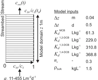
5, 971–1001, 2008 Contaminant mass fluxes from streambed sediments C. Schmidt et al. Title Page Abstract Introduction Conclusions References Tables Figures ◭ ◮ ◭ ◮ Back Close Full Screen / EscPrinter-friendly Version Interactive Discussion qz11-455 Lm d -2 -1 c (t)out c /cS0 S 0 1 Kd 1,2-DCB 229.0 Lkg-1 KdMCB Lkg-1 61.3 Kd1,3-DCB Lkg-1 310.8 Kd1,4-DCB Lkg-1 368.8 rbulk kgL-1 1.5 ne - 0.3 Dz m 0.04 Dt d 0.5 Stream Streambed Model domain 1m z c /cS0 S(t )0 Model inputs
Fig. 2. Concept and input parameters of the multi one-dimensional transport model where the release of contaminants is modeled forqz ranging between 11 and 455 Lm−2d−1.
HESSD
5, 971–1001, 2008 Contaminant mass fluxes from streambed sediments C. Schmidt et al. Title Page Abstract Introduction Conclusions References Tables Figures ◭ ◮ ◭ ◮ Back Close Full Screen / EscPrinter-friendly Version Interactive Discussion
Snap-shot sample concentration [µgL-1]
0 2 4 6 8 10 20 40 60 80 100 Dosimeter derived concentration [µg ] L -1 0 2 4 6 8 10 20 40 60 80 100 groundwater surface water Ceramic dosimeter vs. concentrations from Kalbus et al. 2007 MCB 1,2-DCB 1,3-DCB 1,4-DCB Surface water Groundwater
Streambed high discharge Streambed low discharge
Ceramic dosimeter vs. snap-shot sample derived concentrations
Fig. 3. Comparison of snap-shot sampling and ceramic dosimeter derived aqueous concentra-tions of MCB and DCBs in different compartments (surface water, groundwater, streambed).
HESSD
5, 971–1001, 2008 Contaminant mass fluxes from streambed sediments C. Schmidt et al. Title Page Abstract Introduction Conclusions References Tables Figures ◭ ◮ ◭ ◮ Back Close Full Screen / EscPrinter-friendly Version Interactive Discussion MCB 1,2-DCB 1,3-DCB 1,4-DCB Distance along Transect [m]
-100 0 100 200 300 400 500 qz []Lm d -2 -1 Aqueous concentration [µgL] -1 Sampler number 5 6 7 8 0 20 40 60 80 100 Array 1 9 10 11 12 Sampler number Aqueous concentration [µgL-1] 0 20 40 60 80 100 Array 2 13 14 15 16 Aqueous concentration [µgL-1] 0 20 40 60 80 100 Sampler number Array 3 Surface water 17 20 Sampler number 0 5 10 15 20 Aqueous concentration [µgL-1] (a) (c) (b) (d) (f) Groundwater 18 19 Sampler number 0 5 10 15 20 Aqueous concentration [µgL-1] (e) 0 25 50 75 100 125 150 175 200
Fig. 4. Average aqueous concentrations of MCB and DCBs derived from the ceramic dosime-ters in the surface water (a), the groundwater (e). Aqueous concentrations in the streambed are plotted for different depths at a low groundwater discharge location (b) and two high ground-water discharge locations (c), (d); along the studied reach with heterogeneous groundground-water discharge patterns (f).
HESSD
5, 971–1001, 2008 Contaminant mass fluxes from streambed sediments C. Schmidt et al. Title Page Abstract Introduction Conclusions References Tables Figures ◭ ◮ ◭ ◮ Back Close Full Screen / EscPrinter-friendly Version Interactive Discussion Time [h] Solid-phase fraction 0.97 0.98 0.99 1.00 0 8 16 24 Time [h] 0.97 0.98 0.99 1.00 MCB 1,2-DCB 1,3-DCB 1,4-DCB 0 20 40 60 80 100 120 140 160 180
Fig. 5. Remaining solid phase fraction of MCB and DCBs in the streambed sediments after two desorption experiments of different duration.
HESSD
5, 971–1001, 2008 Contaminant mass fluxes from streambed sediments C. Schmidt et al. Title Page Abstract Introduction Conclusions References Tables Figures ◭ ◮ ◭ ◮ Back Close Full Screen / EscPrinter-friendly Version Interactive Discussion Time (t ) [years]90 0 200 400 600 800 1000 1200 1400 1600 1800 2000 0 50 100 150 200 250 300 350 400 450 MCB 1,2-DCB 1,3-DCB 1,4-DCB qz []Lm d -2 -1
Average groundwater discharge: 58.2 Lm d-2 -1
Fig. 6. Dependence of the timescales to reduce the concentrations of MCB and DCBs in the discharging groundwater (Cout) by 90% from the initial value on the magnitude of groundwater discharge (qz).
HESSD
5, 971–1001, 2008 Contaminant mass fluxes from streambed sediments C. Schmidt et al. Title Page Abstract Introduction Conclusions References Tables Figures ◭ ◮ ◭ ◮ Back Close Full Screen / EscPrinter-friendly Version Interactive Discussion Time [years] 0 100 200 300 400 500 600 700 800 900 1000 1100 1200 MS (t)/ MS 0 0.1 0.2 0.3 0.4 0.5 0.6 0.7 0.8 0.9 1.0 Heterogeneous groundwater discharge 1,2-DCB 1,3-DCB MCB 1,4-DCB Homogeneous groundwater discharge MCB 1,2-DCB 1,3-DCB 1,4-DCB
Fig. 7. Normalized contaminant mass flow rates along the studied reach for homogeneous and heterogeneous groundwater discharge as a function of time.