HAL Id: hal-00298295
https://hal.archives-ouvertes.fr/hal-00298295
Submitted on 23 Oct 2006
HAL is a multi-disciplinary open access
archive for the deposit and dissemination of
sci-entific research documents, whether they are
pub-lished or not. The documents may come from
teaching and research institutions in France or
abroad, or from public or private research centers.
L’archive ouverte pluridisciplinaire HAL, est
destinée au dépôt et à la diffusion de documents
scientifiques de niveau recherche, publiés ou non,
émanant des établissements d’enseignement et de
recherche français ou étrangers, des laboratoires
publics ou privés.
Plastic sea ice rheology in HadCM3
W. M. Connolley, A. B. Keen, A. J. Mclaren
To cite this version:
W. M. Connolley, A. B. Keen, A. J. Mclaren. Results from the implementation of the Elastic Viscous
Plastic sea ice rheology in HadCM3. Ocean Science, European Geosciences Union, 2006, 2 (2),
pp.201-211. �hal-00298295�
Results from the implementation of the Elastic Viscous Plastic sea
ice rheology in HadCM3
W. M. Connolley1, A. B. Keen2, and A. J. McLaren2
1British Antarctic Survey, High Cross, Madingley Road, Cambridge, CB3 0ET, UK 2Met Office Hadley Centre, FitzRoy Road, Exeter, EX1 3PB, UK
Received: 13 June 2006 – Published in Ocean Sci. Discuss.: 10 July 2006
Revised: 21 September 2006 – Accepted: 16 October 2006 – Published: 23 October 2006
Abstract. We present results of an implementation of the
Elastic Viscous Plastic (EVP) sea ice dynamics scheme into the Hadley Centre coupled ocean-atmosphere climate model HadCM3. Although the large-scale simulation of sea ice in HadCM3 is quite good with this model, the lack of a full dynamical model leads to errors in the detailed representa-tion of sea ice and limits our confidence in its future predic-tions. We find that introducing the EVP scheme results in a worse initial simulation of the sea ice. This paper documents various enhancements made to improve the simulation, re-sulting in a sea ice simulation that is better than the original HadCM3 scheme overall. Importantly, it is more physically based and provides a more solid foundation for future devel-opment. We then consider the interannual variability of the sea ice in the new model and demonstrate improvements over the HadCM3 simulation.
1 Introduction
Sea ice is an important aspect of polar climate and strongly affects the ocean-atmosphere exchange of heat. Moreover, it can be used as a diagnostic of climate change in the polar regions. Hence it is desirable to have a physically realis-tic sea ice model within any state-of-the-art global climate model, both to interpret hindcasts and to have confidence in forecasts. The Hadley Centre coupled ocean-atmosphere climate model HadCM3 (Gordon et al., 2000) has sea ice dynamics implemented as an “ocean drift” model in which the sea ice moves with the top level of the ocean. This is better than static sea ice but, physically, amounts to ne-glecting all terms except the water stress in the sea ice dy-namics equation. Although the large-scale simulation of sea ice in HadCM3 is quite good with this model, the lack of
Correspondence to: W. M. Connolley
a full dynamical model incorporating wind stresses and in-ternal ice stresses leads to errors in the detailed representa-tion of sea ice and limits our confidence in its future predic-tions. Accordingly we decided to implement a full dynami-cal model into HadCM3, and chose the EVP model of Hunke and Dukowicz (1997) because of its excellent parallel scaling properties and ease of implementation.
Simply swapping in the EVP scheme results in a worse initial simulation of the sea ice. Hence we present sensitivity studies of the effects of variations of the ice strength param-eter and modifications to the ocean-ice heat flux paramparam-eteri- parameteri-sation designed to improve the simulation. The end result is a sea ice simulation that is better than the original HadCM3 scheme overall, with improvements in some seasons and ar-eas and deficiencies in others. However, it is much more physically based and provides a more solid foundation for future improvement.
As an example of the behaviour of the new model, we consider the interannual variability of the sea ice area. In HadCM3 (and many other GCMs, as shown by Holland and Raphael, 2006) the interannual variability of the sea ice area is overestimated; in the new model the variability is well re-produced, as is the seasonal cycle of variability. Finally we note that various sources of error are present in the coupled model system that would preclude a perfect sea ice simula-tion even from a perfect sea ice model.
2 The models: HadCM3, “Ocean drift” and EVP
2.1 HadCM3
The HadCM3 climate model is the Hadley Centre coupled ocean atmosphere sea ice model, version 3, as used in the IPCC Third Assessement Report. This has a horizontal reso-lution of 2.5◦latitude by 3.75◦longitude for the atmospheric component and 1.25◦by 1.25◦in the oceans. There are 19
levels in the atmosphere and 20 vertical levels in the ocean. Further details are given by Gordon et al. (2000); the sea ice in particular is described by Turner et al. (2001); and the Antarctic climate is described by Turner et al. (2006). The sea ice component uses the zero-layer thermodynamics model of Semtner (1976), and a primitive dynamic scheme called “ocean drift” whereby the sea ice moves with the top level ocean layer. Formally, this amounts to neglecting all terms in the momentum equation except for the water stress. In order to prevent the formation of excessively thick ice, a “convergence limiter” is used to prevent convergence when ice is more than 4 m thick. This could be considered as a primitive rheology. In practice, there is a close relation be-tween the wind and water stresses on the average, so the scheme performs better than might be expected. But there are obvious deficiencies to the scheme, especially near land, where the wind stress can be directly offshore (and frequently is around Antarctica in both reality and the model) whereas the ocean currents generally flow parallel to the coast .
2.2 The Elastic Viscous-Plastic rheology
The EVP rheology is described by Hunke and Dukowicz (1997). It incorporates full viscous-plastic rheology as in Hibler (1979), with an elastic component for computational purposes to permit time-stepping. The elastic waves should be removed during the EVP sub-time-stepping; this has been verified in this implementation. The momentum equation used is
mdui/dt = aτa−aτw−k × mf ui+τi (1)
where m is the combined mass of ice and snow, ui is the ice
velocity, a is the ice concentration, k is a unit vertical, τais
the wind stress on the ice provided by the standard parametri-sation from the atmospheric component HadAM3 (Pope et al., 2000), τw is the ocean drag on the ice, f is the Coriolis
parameter and τi represents the internal stress of the ice as
calculated by the EVP scheme. All the terms are expressed per unit area of the grid box (not per unit area of ice; Con-nolley et al., 2004). The ice-ocean stress τwis parameterised
as cwρw|ui−uw|(ui−uw), with cwthe ice-ocean drag
coef-ficient (0.0055, Kreyscher et al., 2000), ρw the density of
seawater and uwthe surface ocean velocity.
EVP was designed to be implemented in a parallel context and scales well, and so is particularly suitable for use in in HadCM3. The EVP scheme implemented in HadCM3 uses the ice strength parameterization of Hibler (1979), where the pressure, P, a measure of the ice strength depends on both ice thickness and fraction: P=P*ahexp(-c*(1-a)); where a is the ice fraction, h the ice thickness, c* a dimensionless parame-ter with value 20, and P* we use as a tuneable parameparame-ter for the ice strength.
2.3 The ice-ocean heat flux
The standard HadCM3 parameterisation for the grid box mean (GBM) ice-ocean flux, F , is based solely on the tem-perature difference between the topmost ocean layer and the sea ice,
F = (Kρwcp/0.5d) × (To−Tf) (2)
where the diffusivity, K, is 2.5×10⁻⁵m2s−1, cp is the
spe-cific heat of seawater, the first ocean level has temperature
Toand depth d (10 m) and Tf is the basal sea ice
tempera-ture (i.e. the freezing temperatempera-ture of sea water which is set to
−1.8◦C) .
As shown in Eq. (2) above, the default parameterisation of the GBM ocean to ice heat flux in HadCM3 is inde-pendent of the ice concentration. This works well within HadCM3, but clearly owes more to simplicity than physi-cal reality. A more physiphysi-cal version, referred to here as the “P-scheme” (P for proportional), increases the diffusivity, K, from 2.5×10⁻⁵m2s−1to 2.5×10⁻⁴m2s−1(in better agree-ment with observations; McPhee et al., 1999) and makes the heat fluxes proportional to the ice fraction.
A more physically based parameterisation would include the effects of turbulence via the ice-ocean velocity shear. This cannot be done in the ocean drift version because the ice moves with the same velocity as the ocean. Based upon McPhee (1992) and analogy with the atmospheric model parametrisation of the surface flux we write
F = (Kρwcp/0.5d) × (To−Tf) × |uw−ui|/C (3)
where K is the diffusivity and C is a tuning constant with units of velocity. When the ocean-ice shear is above C, the new parameterisation results in more heat flux from the ocean into the ice, tending to melt the ice. From McPhee (1992), a value of 0.1 m s−1is reasonable for C, although it is not well constrained by available measurements. We shall call this the “M-scheme” generically, or “M C” where C is used as a label for the constant in Eq. (3) , e.g. M 5 when C is 0.05 m s−1.
3 Observations
We compare the model sea ice concentrations against pas-sive microwave satellite (SSMI) observations for years 1979 to 2002. We use the “bootstrap” data of Comiso (2003) since it gives more accurate (higher) concentration values in the Antarctic than the NASA Team algorithm (Comiso and Steffen, 2002; Connolley, 2005). The disagreement between Bootstrap and NASA Team is considerably smaller than be-tween the observations and the model, or different versions of the model. For example in September the Southern Hemi-sphere (SH) mean ice area is 1.5×10¹³m2in NASA team but 1.6×10¹³m2in Bootstrap.
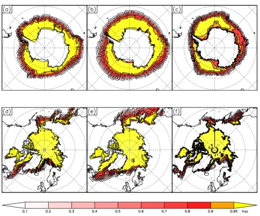
Fig. 1. Sea ice concentration at maximum extent from HadCM3, initial HadCM3+EVP and observations (a–c): September in the SH; (d–f): March in the NH. (a, d): HadCM3; (b, e): HadCM3+EVP; (c, f): Observations.
4 Experiments
We shall show results from the standard HadCM3 run, and the results of implementing EVP and the physical modifi-cations described above. These experiments are labeled as shown in Table 1.
All of the model runs used here begin from the same stan-dard HadCM3 dump taken from the control run, which has greenhouse gas forcing appropriate to pre-industrial levels. The “HadCM3” results here are thus a continuation of the control run, and no spin up is required. The various EVP runs have the first 5 years discarded for spin up, and then 20 years of run are used to smooth out interannual variations.
5 Results
5.1 EVP in HadCM3
Figure 1 compares the HadCM3 sea ice to observations from SSMI for the winter period. Overall the simulation compares well with observations, however the total extent of the model ice is slightly too big and there are regions of large differ-ences, especially from 40 E to 140 E in the SH, to the west of the Antarctic Peninsula and in the Barents Sea.
Initial implementation of EVP into HadCM3 produces re-sults that are disappointing (Figs. 1 and 2). In winter, the ice
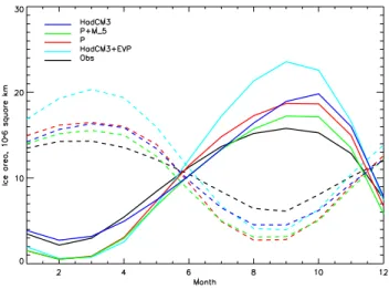
Fig. 2. Annual cycle of ice area from HadCM3 (blue), HadCM3+EVP (light blue) and observations (black). Solid lines: SH; dashed lines: NH.
area of HadCM3 was greater than observations in both hemi-spheres, and adding EVP makes it even greater. In summer, in the SH, the ice area in HadCM3 compares well with obser-vations; but adding EVP reduces the model ice area. In the Northern Hemisphere (NH), the summer area was too small, and adding EVP does not change this. EVP improves the
Table 1. HadCM3 experiments.
Experiment name Experiment details
HadCM3+EVP HadCM3, with the EVP scheme added; the initial default value for the ice strength parameter P* is 27×103N m−2
HadCM3+M C HadCM3+EVP plus the shear-dependent ocean-ice heat flux M-scheme, where
Cis the constant in Eq. (3). Note that the “+EVP” label is not required, since this scheme cannot be implemented within the standard HadCM3 framework HadCM3+P HadCM3+EVP plus the P-scheme where the ocean-ice heat flux is
propor-tional to ice concentration and the diffusivity is increased to 2.5×10⁻⁴m2s−1 HadCM3+P+M C HadCM3+EVP plus the P-scheme and M-scheme
HadCM3+P+M C P* X HadCM3+ P+M C plus variations in the ice strength parameter P* (X=5, 10, 27 and 100×103N m−2)
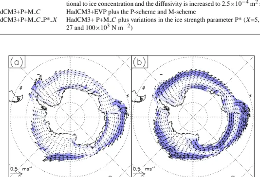
Fig. 3. Sea ice velocity in September from (a) HadCM3 and (b) HadCM3+EVP. Lighter shading above 0.05 ms−1; darker above 0.1 ms−1.
simulation in some respects around Antarctica: the ice in the Bellingshausen Sea close to the Antarctic Peninsula in now more extensive and more concentrated. The lack of ice in this region in the standard HadCM3 run hinders interpreta-tion of climate change in the Antarctic Peninsula, which is closely linked to the sea ice (King, 1994). Also, the phase of the maximum in ice area in the SH is placed correctly in September in EVP whereas it was in October in HadCM3.
The dynamic sea ice rheology substantially affects the ice velocities (Fig. 3). In the SH speeds are faster with EVP although the broad scale pattern is similar. The fastest ice occurs around the coast of East Antarctica in response to the coastal easterlies, and towards the edges of the pack in the zone of westerlies. By including the wind stress directly, EVP allows offshore advection of ice in the Ross Sea area, and produces a better-defined sea ice flow in the Weddell gyre, in better agreement with observations. In the NH (not shown) the effects within the Arctic Basin are less, though ice speeds increase in the Bering Strait and along the east coast of Greenland. The ice flow export through the Fram Strait is realistic, but the flow within the Central Arctic basin
is not. This is largely due to the wind stress forcing: the model (as with the basic HadCM3) simulates too-high Mean Sea Level Pressure (MSLP) over the Central Arctic, and the Icelandic low is not deep enough. A lesser problem is the ocean circulation, which cannot be fully realistic due to the presence of a “polar island” introduced for numerical rea-sons, since the ocean model is on a regular grid. (Note that although the ocean must flow around the island, the sea ice may flow over it; however the ocean currents are inevitably unrealistic.) For these reasons we focus more on the Antarc-tic simulation from the model.
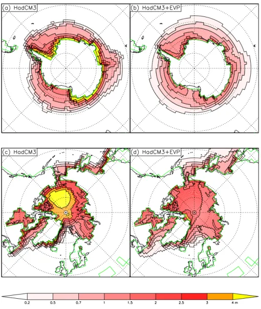
Figure 4 shows the effects of the rheology on the ice thick-ness in winter. In general the ice becomes thinner, as would be expected, since the rheology acts to decrease thickening by convergence. Also, the wind forcing in the SH drives ice away from the coast which reduces the thickness. In the SH, the ice thickness in the eastern sector is improved rela-tive to the limited observations available (Timmermann et al., 2004) especially along the coast. However, the ice is now too thin in the western sector in HadCM3+EVP. The ice thick-ness is also too low in the Arctic compared with observations
Fig. 4. Ice thickness for (a) HadCM3 (b) HadCM3+EVP for the SH; (c, d) the same, for the NH.
(Bourke and Garrett, 1987; Laxon et al., 2003). The observa-tions show the thickest ice is banked up against the northern coasts of Greenland and the Canadian Archipelago. This is not achieved in HadCM3+EVP due to the errors in the wind forcing.
The degradation of some aspects of the simulation by adding EVP should not be too surprising as several of the thermodynamic parameterisations of HadCM3 had been de-veloped and tuned with the existing ocean drift sea ice model. Hence, we next examine the effects of some physically based improvements to the thermodynamic parameterisations on the simulation.
5.2 The ice-ocean heat flux
We present results of the M-scheme, in which the ice-ocean flux is made proportional to the velocity shear between the
ice and the ocean. This ocean-ice shear is highest near the edge of the pack, where the ice moves fastest, with values above 0.2 m s−1; is above 0.1 m s−1 in much of the pack, declining to below 0.05 closer to the coast. Figure 5 shows the difference in sea ice area compared to the initial HadCM3+EVP run with values of C of 0.05 and 0.1 m s−1. The new parameterisation makes a substantial contribution to reducing the difference between the observed and model ice areas in winter, although the summer areas are slightly worse in the Arctic.
We attempted to “tune” the model by adjusting the value of C within the physically reasonable range. However, whilst changes do have an effect, there is a trade-off between sum-mer and winter ice; decreasing C reduces the winter ice area to more realistic values, but also decreases the summer ice to undesirably low values. We settled upon a value of 0.05 m s−1.
Fig. 5. Response of ice area to variation in the ice-ocean heat flux. Black, observations; Blue, HadCM3; light blue, HadCM3+EVP; Red, HadCM3+M 10; Green, HadCM3+M 5. Solid lines: SH; dashed lines: NH.
Fig. 6. Response of ice area to variation in the ice-ocean heat flux P scheme. Black, observations; Blue, HadCM3; light blue, HadCM3+EVP; Red, HadCM3+P; Green, HadCM3+P+M 5. Solid lines: SH; dashed lines: NH.
Further improvements are found with the P-scheme, in which the ice-ocean flux becomes proportional to the ice area and the diffusivity is increased. Over marginal ice with a low fraction this is a near-neutral change; where the ice has a high fraction this potentially increases the ocean-ice flux and hence the ice melting. However the effect is not as large as might be expected because it is limited by the heat capac-ity of the ocean underneath the ice; this has been tested by increasing the diffusivity further, where it makes little differ-ence. The P-scheme has a major impact on the simulation (Fig. 6), particularly on the winter ice where the ice area in both hemispheres is reduced back down to standard HadCM3 levels and much better agreement with observations. In
sum-Fig. 7. Response of ice area to variation in P*. Black, observations; Blue, HadCM3. Purple, light green, red and light blue are, respec-tively, P*=0, 5, 27 and 100×103N m−2in HadCM3+P+M 10+P*. Solid lines: SH; dashed lines: NH.
mer, there is little effect in the SH whereas the area reduces in the NH. Either P or M scheme results in significant changes to the sea ice area; Fig. 6 also shows both schemes combined as HadCM3+P+M 5 which results in a further slight reduc-tion in the ice area.
Further improvements to the thermodynamics model or more experiments with tuning the thermodynamics could well be desirable, but are outside the scope of this paper 5.3 Varying the ice-strength parameter P*
Implementations of the Viscous-Plastic and EVP rheolo-gies have tended to standardise around a value of 27×103 N m−2 for P* (Hibler, 1979) but a range of values are used. In ocean-ice models forced by observed atmospheric fields, it is common to tune P* by comparing against buoy data (or against observed ice thickness and other parame-ters (Miller at al., 2005)); that method is not possible in a coupled ocean-atmosphere-seaice model and it may well be resolution-dependent. We investigate the influence of the choice of P* on the simulation and find that higher values of P* tend to lead, in the SH, to more winter ice and less summer ice: see Fig. 7; as the ice becomes less compress-ible with higher P* it is pushed further out. The sensitiv-ity to P* in this case is quite small – considerably smaller than the sensitivity to changes in the thermodynamic param-eters. These runs are variations around the base state of HadCM3+P+M 10. Greater sensitivity, with changes in the same sense (i.e. higher P* leading to more winter ice) is seen in runs using plain HadCM3+EVP as the base state – without the thermodynamic modifications detailed above.
In summer, in the SH, the (unreasonably high) value of P*=100×103N m−2causes all the summer ice to disappear, which is unrealistic. Based on the SH results, one would
tion. Based on these results and the range of values in the literature, we choose a value of 5×10³N m−2for P*; which is the value used in Miller et al. (2005).
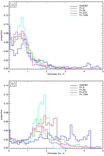
Figure 8 shows histograms of the seaice thickness for var-ious values of P*. As expected, higher values of P* make the ice less compressible and hence more ice is of lower thick-ness. This is more noticeable in the NH, where rheology is more important. For P*=0 in the NH there is a long “tail” of ice of very high thickness, since the ice has no strength. By comparison, the HadCM3 thickness histogram is very dif-ferent, again reflecting the lack of a proper rheology in that model.
6 Optimised EVP run
Combining all the changes, we come to the optimised EVP run as follows:
– McPhee ocean to ice heat flux with C=0.05 m s−1, scaled by the ice concentration and with K=2.5×10⁻⁴m2s−1
– P*=5×10³N m−2
Of the changes, adding the improved (EVP) dynamics has a substantial effect on the sea ice simulation. Having done that, further tuning of the dynamics (via plausible values for P*) has comparatively little effect, as shown by Fig. 7. Tun-ing the thermodynamics has rather larger effects. We have chosen to optimise the model based principally on the SH ice concentration. A different set of parameters may be more appropriate for optimising other fields such as NH ice thick-ness.
The remainder of the paper shows results from this opti-mised run. Maps of the maximum and minimum ice extent for this run are shown in Fig. 9 and the winter ice thickness in Fig. 10. This run has better (reduced) winter sea ice area in both hemispheres compared to HadCM3 (compare Figs. 9 and 1), particularly in the Southern Hemisphere where the concentration is reduced at the ice edge in the Indian and Pacific Ocean sectors. In both hemispheres there is too lit-tle ice in the summer, although HadCM3 had a band of too concentrated ice around much of the Antarctic coastline in the summer which is improved when EVP is included. The seasonal cycle remains too large.
In the optimised run the Central Arctic ice thickness is improved with respect to the initial HadCM3+EVP experi-ment (Fig. 10). The ice is now thicker in the western sector of the Central Arctic, in closer agreement with observations (Bourke and Garrett, 1987; Laxon et al., 2003). However, as already stated the observed spatial pattern of ice thickness
Fig. 8. Histogram of sea ice thickness in September (Antarctic, top) and March (Arctic, bottom). Blue, HadCM3. Purple, light green, red and light blue are, respectively, P*=0, 5, 27 and 100×103 N m−2in HadCM3+P+M 10+P*.
cannot be reproduced because of errors in the wind stress forcing. In the Antarctic the improvements in the Eastern sector seen by introducing EVP have been maintained. The ice in the Western sector remains too thin.
7 Stress balance in the model
We now consider the balance of forces within the sea ice. Figure 11 shows a snapshot of this for a typical day in the SH. As noted above in Sect. 5.1, there are deficiencies in the NH simulation (largely unrelated to the sea ice model itself) so we do not show the NH. The main terms in the bal-ance for the Antarctic are the wind and water stresses; the Coriolis force is weaker, and the internal stresses in general weaker still. Much of the Antarctic ice is close to free-drift balance; exceptions to this are in the Weddell Sea and around the coastlines. The existence of the free-drift balance is not surprising, since the ice is generally unconstrained by land
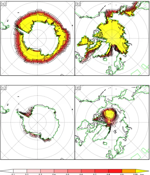
Fig. 9. Sea ice concentration at winter maximum in the optimised run HadCM3+P+M 5+P*5K, (a) SH in September and (b) NH in March; and at summer minimum for (c) SH in March and (d) NH in September.
boundaries and often in divergent flow. However, the inter-nal stress component of the force balance is still important in influencing the ice behaviour on the large scale: as Fig. 7 shows, the total ice area is sensitive to changes in the inter-nal ice strength parameter, P*. In the Arctic, the dominant balance is still between wind and water stresses, but the in-ternal force is larger and significant across the basin. Because of atmospheric circulation errors (not shown) the maximum ice thickness is in the Central Arctic (Fig. 10) rather than against the Canadian Archipelago as it should be; this in turn means that the largest internal ice stresses are not in the cor-rect place.
8 Effects on variability
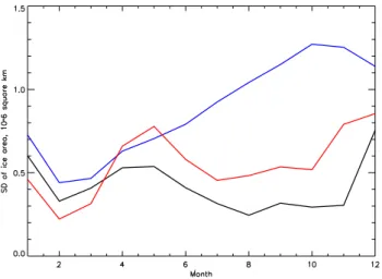
Holland and Raphael (2006) note that the variability of sea ice around Antarctica in climate models is significantly larger than in the observations. For September in the Antarc-tic, over the period 1979–2002, the standard deviation (SD, in 106km2)of ice area of the SSMI observations is 0.32. HadCM3 gives a substantially larger value, 1.13. The op-timized EVP experiment has a variability that matches the observations. Looking at the variability throughout the year, the picture (see Fig. 12) becomes more interesting.
EVP correctly reproduces the form of the curve, with max-ima in January and April and minmax-ima in February and Au-gust. EVP is somewhat too variable, especially at times of larger ice extent. By contrast, HadCM3 has completely the wrong pattern of variability throughout the year, and shows far too much variability, especially in winter and spring.
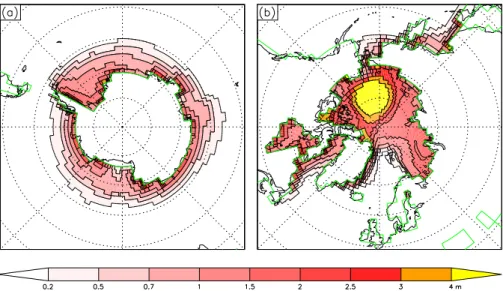
Fig. 10. Sea ice thickness at winter maximum in the optimised run HadCM3+P+M 5+P*5K, (a) SH in September and (b) NH in March.
Fig. 11. Ice velocity and force terms in the momentum equation for a typical winter day, from the optimised EVP experiment (a): ice velocity. (b): wind stress; (c): ice-ocean stress; (d): Coriolis force; (e) internal stress, weighted as in the momentum Eq. (1). Note the changes of scale between the plots.
A different way of examining the variability is to look at the standard deviation of the ice cover, point-wise. For September, this has total values (106km2)of 2.5, 3.2, 2.3 for the observations, HadCM3 and EVP, respectively. These
numbers are larger than the SD of the area-total ice area, be-cause they include variations in the ice pattern (if the vari-ability were purely that the ice anomalies rotated around the continent without changing overall area, for example, then
Fig. 12. Interannual standard deviation of total ice area in the SH by month. Black: observations; blue: HadCM3; red: optimized EVP experiment.
the SD of total ice area would be zero, but the total of the ice SD would be non-zero). These values imply that HadCM3 has more variability in spatial location of the anomalies than the observations or EVP. This is confirmed by EOF analysis (not shown): the first EOF of the observations, and EVP, have their variance largely confined to the sector [145◦W, 0◦E]
whereas HadCM3 has large variance between [0◦E, 135◦E]. For the Arctic (not shown) variability is around 0.4×10⁶km2 year-round; HadCM3 reproduces this both with and without EVP. This may be because of the different dynamics dominating in the land-locked Arctic basin.
9 Other sources of error in the sea ice model
In a coupled model, even a perfect sea ice model would not produce a perfect simulation due to deficiencies in other model components. We are not in a position to closely ex-amine deficiencies in the ocean model, but there exist large MSLP errors in HadCM3 (Fig. 13) which imply errors in the wind stress forcing of the sea ice model (as found by Bitz et al., 2002). The largest error is a northwards wind stress at around 90◦E, which is consistent with the excess ice at this longitude within this model. The southwards error in the Amundsen-Bellingshausen sea is compatible with the deficit of sea ice there. The MSLP errors appear to be related to the tropical sea surface temperature errors in HadCM3, in partic-ular those near Indonesia (Lachlan-Cope et al., 20061) and not strongly related to local conditions. Hence they cannot readily be cured, and the sea ice simulation must be evalu-ated in the context of these errors.
1Lachlan-Cope, T. A., Connolley, W. M., and Turner, J.: The
effects of tropical sea surface temperature errors on the Antarctic atmospheric cicrulation of HadCM3, Geophys. Res. Lett., submit-ted, 2006.
Fig. 13. Geopotential height difference at 500 hPa between HadCM3 and ERA, together with implied geostrophic wind anoma-lies.
10 Conclusions
This paper has documented the implementation of the Elas-tic Viscous PlasElas-tic sea ice rheology within the coupled ocean-atmosphere climate model HadCM3. We show that this more physically based rheology nonetheless initially degrades the sea ice simulation, but that a number of the thermodynamic parameterisations relating to the ocean-ice heat flux within the default HadCM3 sea ice scheme can also be improved, and following this the overall sea ice simulation is generally better than HadCM3. Also, since it is now more physically based, we have more confidence in the model both for hind-casts and forehind-casts of climate change. An initial finding is that the interannual variability is in much better agreement with the observations that the original HadCM3 model.
The successor to HadCM3, HadGEM1 (Hadley Centre Global Environmental Model version 1; Johns et al., 2006), uses much the same EVP scheme as here for the dynamics but introduces ice thickness categories to improve the repre-sentation of the ice thermodynamics and ridging. The spa-tial distribution of ice thickness in HadGEM1 is much im-proved in both hemispheres due to the combination of the EVP scheme and more realistic wind forcing (McLaren et al., 2006). Further work on the sea ice model will take place within the framework of the HadGEM model focusing on further improvements to the thermodynamics.
Lipscomb, 2004). Edited by: K. J. Heywood
References
Bitz, C. M., Fyfe, J. C., and Flato, G. M.: Sea Ice Response To Wind Forcing From AMIP Models, J. Climate, 15(5), 522–536, 2002.
Bourke, R. H. and Garrett, R. P.: Sea ice thickness distribution in the Arctic Ocean, Cold Regions Science and Technology, 13, 259– 280, 1987.
Comiso, J.: Bootstrap sea ice concentrations for NIMBUS-7 SMMR and DMSP SSM/I, June to September 2001. Boulder, CO, USA: National Snow and Ice Data Center, Digital media, (http://nsidc.org/data/nsidc-0079.html) 1999, updated 2003. Comiso, J. C. and Steffen, K.: Studies Of Antarctic Sea Ice
Concen-trations From Satellite Data And Their Applications, J. Geophys. Res., 106(C12), 31 361–31 385, 2002.
Connolley, W. M.: Sea ice concentrations in the Weddell Sea: A comparison of SSM/I, ULS, and GCM data, Geophys. Res. Lett., 32(7), L07501, doi:10.1029/2004GL021898, 2005.
Connolley, W. M., Gregory, J. M., Hunke, E., and McLaren, A. J.: On the consistent scaling of terms in the sea-ice dynamics equation, J. Phys. Oceanogr., 34(7), 1776–1780, 2004.
Gordon, C., Cooper, C., Senior, C. A., Banks, H., Gregory, J. M., Johns, T. C., Mitchell, J. F. B., and Wood, R. A.: The Simu-lation Of Sst, Sea Ice Extents And Ocean Heat Transports In A Version Of The Hadley Centre Coupled Model Without Flux Ad-justments, Clim. Dyn., 16(2–3), 147–168, 2000.
Hibler, W. D.: Dynamic thermodynamic sea ice model, J. Phys. Oceangr., 9(4), 815–846, 1979.
Holland, M. M. and Raphael, M. N.: Twentieth century simula-tion of the southern hemisphere climate in coupled models. Part II: sea ice conditions and variability, Clim. Dyn., 26, 229–245, doi:10.1007/s00382-005-0087-3, 2006.
Hunke, E. C. and Dukowicz, J. K.: An Elastic-Viscous-Plastic Model For Sea Ice Dynamics, J. Phys. Oceangr., 27(9), 1849– 1867, 1997.
Hunke, E. C. and Lipscomb, W. H.: CICE: The Los Alamos Sea Ice Model, documentation and software, Version 3.1, LA-CC-98-16, Los Alamos Natl. Lab., Los Alamos, N.M., 2004.
Gregory, J. M., Keen, A. B., Pardaens, A. K., Lowe, J. A., Bodas-Salcedo, A., Stark, S., and Searl, Y.: The new Hadley Centre climate model HadGEM1: Evaluation of coupled simulations, J. Climate, 19(7), 1327–1353, 2006.
King, J. C.: Recent Climate Variability In The Vicinity Of The Antarctic Peninsula, International Journal Of Climatology, 14(4), 357–369, 1994.
Kreyscher, M., Harder, M., Lemke, P., and Flato, G. M.: Results of the Sea Ice Model Intercomparison Project: Evaluation of sea ice rheology schemes for use in climate simulations, J. Geophys. Res., 105(C5), 11 299–11 320, 2000.
Laxon, S., Peacock, N., and Smith, D.: High interannual variability of sea ice thickness in the Arctic region, Nature, 425(6961), 947– 950, 2003.
McLaren, A. J., Banks, H. T., Durman, C. F., Gregory, J. M., Johns, T. C., Keen, A. B., Ridley, J. K., Roberts, M. J., Lipscomb, W. H., Connolley, W. M., and Laxon, S. W.: Evaluation of the Sea Ice Simulation in a new Coupled Atmosphere-Ocean Climate Model (HadGEM1), J. Geophys. Res. (Oceans), in press, 2006. McPhee, M. G.: Turbulent heat flux in the upper ocean under sea
ice, J. Geophys. Res., 97(C4), 5365–5379, 1992.
Mcphee, M. G., Kottmeier, C. and Morison, J. H.: Ocean Heat Flux In The Central Weddell Sea During Winter, J. Phys. Oceangr., 29(6), 1166–1179, 1999.
Miller, P. A., Laxon, S. W., and Feltham, D. L.: Improving The Spa-tial Distribution Of Modeled Arctic Sea Ice Thickness, Geophys. Res. Lett., 32(18), L18503, doi:10.1029/2005GL023622, 2005. Pope, V. D., Gallani, M. L., Rowntree, P. R., and Stratton, R. A.:
The impact of new physical parametrisations in the Hadley Cen-tre climate model: HadAM3, Clim. Dyn., 16, 123–146, 2000. Semtner, A. J.: A model for the thermodynamic growth of sea ice in
numerical investigations of climate, J. Phys. Oceanogr., 6, 379– 389, 1976.
Timmermann, R., Worby, A., Goosse, H., and Fichefet, T.: Utiliz-ing the ASPeCt sea ice thickness data set to evaluate a global coupled sea ice-ocean model, J. Geophys. Res., 109, C07017, doi:10.1029/2003JC002242, 2004.
Turner, J., Connolley, W. M., Cresswell, D., and Harangozo, S. A.: The simulation of Antarctic sea ice in the Hadley Centre Climate Model (HadCM3), Ann. Glaciol., 33, 585–591, 2001.
Turner, J., Connolley, W. M., Lachlan-Cope, T. A., and Marshall, G. J.: The performance of the Hadley Centre Climate Model (HadCM3) in high southern latitudes, Int. J. Climatol., 26, 91– 112, 2006.