by Zhili Tian
Eng.B. in Civil Engineering (1988) Tsinghua University, Beijing, P. R. China
Submitted to the Department of Civil and Environmental Engineering in partial fulfillment of the requirements for the degree of
Master of Science in Transportation at the
MASSACHUSETTS INSTITUTE OF TECHNOLOGY
September 2002
C 2002 Massachusetts Institute of Technology. All rights reserved.
Signature of A uthor ... .... ...
Department of Civil and Environmental Engineering August 16, 2002 'In
X?
...
.... .. Moshe E. Ben-Akiva Edmund K. Turner Professor of Civil and Environmental Engineering Thesjs Supervisor
... ... .. ..
'"7HarisN. Koutsopoulos Operations Research Analyst Volpe National Transportation Systems Center Thesis Supervisor Accepted by ...
Chairman, epartmental Committee
-...---. Oral Buyukozturk on Graduate Studies MASSACHUSETTS $PJTITIE OF TECHNOLOGY
Lu
19 2002
LIBRARIES
Certified by ... Certified by ...by Zhili Tian
Submitted to the Department of Civil and Environmental Engineering on August
16, 2002 in partial fulfillment of the requirements for the degree of Master of
Science in Transportation
Abstract
This thesis proposes two models that estimate the capacity of an intersection with actuated control. The capacity of an approach to or a lane group of the intersection is a function of the saturation flow rate, the green time allocated to this approach or lane group, and the cycle length of the intersection. The Minimum Delay Model estimates the green times and the cycle lengths from flow rates, minimizing the total delay at the intersection. Parameters, the ratio of green extension period to queue service time specific to each approach or lane group, are introduced into this model. The parameters depend on the distribution of arrivals of vehicles at the intersection. The Hybrid Model combines the deterministic queuing model that estimates the queue service time and a theoretical model that estimates the green extension period from the unit extension, the flow rate, the speed limit of the approach, and the detector length. A method converting the left-turn traffic volume to equivalent through volume is developed. The method is applied to estimating the capacity of intersections with permitted left-turn phases. The Minimum Delay Model and the Hybrid Model are validated at the intersection level by comparing the estimations of effective green ratios with those simulated by MITSIM-Lab. These two models are also validated at the network level with real data from Irvine, California. The results show that both the Minimum Delay Model and the Hybrid model are appropriate for estimating capacity of intersections with actuated control. The Minimum Delay Model is also suitable for estimating capacity of intersections with adaptive control. The Emulation Model is applicable to off-line mesoscopic dynamic traffic assignment.
Thesis Supervisor: Moshe E. Ben-Akiva
Edmund K. Turner Professor of Civil and Environmental Engineering Thesis Supervisor: Haris N. Koutsopoulos
I am indebted to a great number of people who generously offered advise, encouragement, inspiration, and friendship throughout my time at MIT.
I hold my utmost respect and sincere gratitude to my advisor, Prof. Moshe Ben-Akiva and Dr. Haris Koutsopoulos. I thank Moshe for sharing his knowledge, for support, for the opportunities he has provided me, for forcing me dig deeper into my research, his encouragement, and his invaluable ideas. I thank Haris for sharing his knowledge, his friendship, his guidance, his support, his patience, and his selfless commitment.
I thank my fellow students at ITS lab. Thanks to Kunal Kunde, Rama Balakrishna, Srinivasan Sundaram and for their technical aid, friendship and their work on DynaMIT. Thanks to everyone else in the ITS lab for their friendship and kindness.
I thank the faculty and staff of CTS for their dedicated and kindness. Special thanks to Leanne Russell for her kind support.
Finally, my greatest thanks and appreciation go to my family. I thank my family for their permanent love and support. I realize how lucky I am to have them.
Contents
ABSTRACT...3 ACKNOWLEDGEMENT...5 L ist o f T ab les ... 9 L ist o f F igures ... 10 CHAPTER 1 INTRODUCTION...111.1 Scope of the T hesis...12
1.2 C on tribution s ... 12
1.3 T hesis O rganization ... 12
CHAPTER 2 LITERATURE REVIEW ... 14
2 .1 In trodu ction ... ...--- 14
2 .2 Pretim ed C ontrols...14
2 .3 A ctuated C ontrols...15
2.3.1 N E M A C ontroller ... 16
2.3.2 Tim ing C haracteristics ... 18
2 .4 A daptive C ontrol ... 20
2.4.1 Traffic-Responsive System (SCOOT) ... 21
2.4.2 Optimized Policies for Adaptive Control...23
2.5 Methods for Estimating the Capacity of Traffic-Actuated Intersections...25
2 .5.1 A llsop 's M ethod...26
2.5.2 D aganzo's M ethod ... 27
2.5.3 Highway Capacity Manual Methodology ... 29
2.5.4 Traffic Control System Handbook...33
CHAPTER 3 CAPACITY ESTIMATION OF APPROACHES TO ISOLATED INTERSECTIONS WITH TRAFFIC-ACTUATED CONTROL...34
3.1 The M inim um D elay M odel... 34
3 .1.1 A ssum p tion s...34
3.1.2 Determination of the Intersection Capacity by Minimizing the Total Delay... 35
3.1.3 Expressions of Cycle Length and Green Times ... 39
3.1.4 Reformulation of the Optimization Problem in terms of cLi and yj...43
3.1.5 Comments on the Minimum Delay Model...45
3.2 T he H ybrid M odel ... 45
3.3 Treatment of Left-turn flow Rates in Capacity Estimation ... 47
CHAPTER 4 IMPLEMENTATION OF CAPACITY ESTIMATION MODELS IN DYNAMIT 49 4.1 Introduction to DynaMIT ... 49
4.2 Implementation of the Minimum Delay Model and the Hybrid Model ... 51
4.2.1 Averaging the Lane Group Capacities ... 52
4.2.2 Input Data for the Capacity Estimation Models...53
4.3 Imposing Lower Bound on Green Times and Initial Lane Group Capacities ... 53
CHAPTER 5 VALIDATION OF THE PROPOSED MODELS...54
5.1 Validation of the Proposed Models at Intersection Level ... 54
5.1.1 Introduction to the Two Intersections ... 54
5.1.2 Comparison of the Proposed Models with those from TCS Handbook...57
5.1.3 Comparison of the Green Times Estimated by Proposed Models with those simulated by MITSIM-Lab at An Intersection with Eight Protected Phases ... 59
5.1.4 Comparison of the Green Time Estimations by Different Models at An Intersection
with Permitted Left Turn Phases... 64
5.2 Validation of the Capacity Estimation Models at Network Level...67
5 .2 .1 Introdu ction ... 67
5.2.2 Comparison of the Field Observations and the Simulated Flows ... 68
5 .2 .3 E rror Statistics...69
5.3 V alidation C onclusion ... 70
CHAPTER 6 CONCLUSION AND FUTURE STUDY ... 71
6 .1 C on clu sion ... 7 1 6 .2 F uture Study ... 72
APPENDIX A GREEN TIMES AND CYCLE LENGTH FOR N PHASES...73
1. The Relationship between X and y2 for Approach 2 ... 73
2. The Cycle Length and Green Times for An Intersection with n Phases ... 73
3. Correctness of the Minimum Delay Model ... 75
APPENDIX B ... 78
1. Representation of C in Terms of ai, a2, y1, and y2... . . . 78
2. Representation of d, in Terms of a1, a2, y1, and y2... . . . . .. . . . 78
3. Representation of dr in Terms of a1, a2, y1, and y2... . . . . 79
APPENDIX C INPUT DATA OF CAPACITY ESTIMATION ... 81
1. Determining Protected Left-turn or Permitted Left-turn Phases ... 81
2. Preparation of Input Data for Actuated Control ... 82
List of Tables
Table 5-1 Saturation Flow Rates (vphg)... 56
Table 5-2 Saturation Flow Rates (vphg)... 57
Table 5-3 Comparison of Timing Plans Estimated by Four Different Models...58
Table 5-4 Flow Rates into the Intersection ... 61
Table 5-5 Effective Green Ratios Estimated by Different Models under Different Scenarios at Intersection of Irvine Center Dr and Laguna Cyn... 61
Table 5-6 Flow Rates into the Intersection...64
Table 5-7 Comparison of Effective Green Ratios Estimated by Different Models under Different Scenarios at the Intersection with Permitted Left-turn Phases...65
List of Figures
Figure 2.1 Four-phase Controller Diagram 16
Figure 2.2 Eight-phase (dual-ring) Controller Diagram 17
Figure 2.3 Phase Order for Dual-ring Controller 17
Figure 2.4 Actuated Phase Intervals 18
Figure 2.5 A Gap-reduction Function 20
Figure 2.6 The Actuated Traffic Signal Strategy under which Green Phases Terminate as soon as
their Queues Vanish 28
Figure 2.7 Queue Accumulation Polygon Illustrating Green Time Computation 30
Figure 3.1 Intersection Layout 34
Figure 3.2 Signal Phases 35
Figure 3.3 Queue Accumulation Polygon 37
Figure 3.4 Traffic Actuated Control Strategy 40
Figure 4.1 Structure of DynaMIT 49
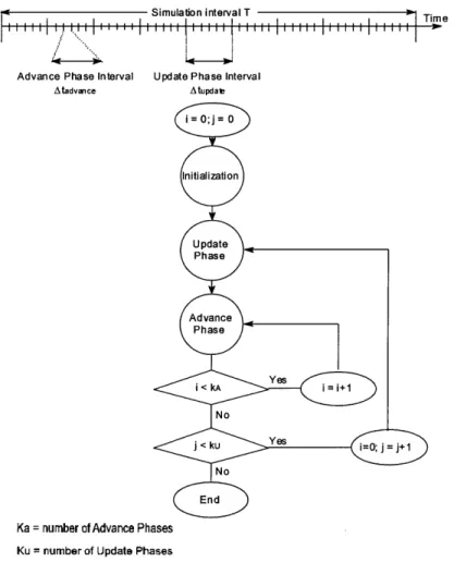
Figure 4.2 Simulation Process 50
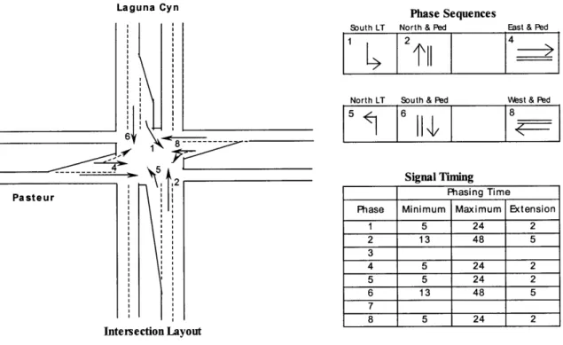
Figure 5.1 Intersection of Irvine Center Dr and Laguna Cyn (Protected Phasing) 55 Figure 5.2 Intersection of Pasteur @ Laguna Cyn with One Permitted Left Turn Phase 55
Figure 5.3 Heavy Traffic Volume 62
Figure 5.4 Normal Traffic Volume 62
Figure 5.5 Light Traffic Volume 63
Figure 5.6 Heavy Traffic Volume 65
Figure 5.7 Normal Traffic Volume 66
Figure 5.8 Light Traffic Volume 66
Figure 5.9 Irvine Road Network 67
Figure 5.10 Field Observations v.s. Simulated Flows at Sensor 46 68
Figure 5.11 Field Observations v.s. Simulated Flows at Sensor 47 69
Chapter 1 Introduction
Urban traffic congestion is currently severe in most cities in the world and intelligent transportation systems are being designed to provide real-time control and route guidance to motorists to optimize traffic network performance. Actuated control polices and adaptive control strategies are becoming popular because of their potential to reduce delays at intersections. The advent of extremely fast methods of communication and computation in the past decade has created many new opportunities for controlling traffic on road networks. New control system such as SCOOT, a traffic-responsive system, was developed in the U.K. for optimizing network traffic performance. New control algorithms such as Optimized Policies for Adaptive Control (OPAC), an on-line traffic signal timing optimization algorithm, were developed in the U.S.
Improvement of the traffic control of congested networks progresses slowly because of lack of understanding of the long-term dynamical system within which the traffic control system is embedded. In a congested network with traffic signals controlled automatically according to actuated or adaptive control policy, there are interactions between traffic and signal controls on the various streets. In reality, these interactions are often extremely complicated and their medium-term effects are hard to forecast. Dynamic traffic assignment (DTA) models have been applied to simulating the within-day dynamics of traffic, drivers' route choice, and dynamic traffic control.
In recent research of dynamic traffic assignment, researchers studied impacts of actuated control or responsive control on travelers' route choice and how drivers respond to traffic control. The current research on dynamic traffic assignment focuses on the realistic representation of the traffic network including formulating various actuated or adaptive traffic control. Most of the studies approximate the responsive traffic control by formulating delays on streets with actuated or adaptive traffic control. Since the real-world traffic controls are sophisticated, delay models cannot take into account the various control policies. In this research, we directly estimate the capacity of approaches to intersections with various traffic controls in dynamic traffic assignment.
The capacity of an approach to an intersection with traffic actuated or adaptive control is a function of the flow rates on approaches to the intersection. Since traffic demands are time-dependent, the capacities of intersections with signal control responding to traffic also vary. Intersection capacities estimated from historical demands do not reflect the variations of capacity within a day. Although capacity estimation for intersections with pre-timed control has been comprehensively studied and estimation models exist in the literature, those models cannot be used in estimating capacity of intersections with actuated or adaptive control. For instance, Webster's model is commonly used for designing timing plans of pretimed control. However, this model is not sensitive to the design parameters of actuated control (Courage, 1998). Therefore, the capacity estimation models for pretimed control cannot be used to determine the capacities of actuated intersections in dynamic traffic assignment (DTA).
The traffic controls are oversimplified in dynamic traffic assignment because the traffic-controlled intersections are usually treated as pre-timed. For example, DynaMIT uses the pre-determined approach capacities calibrated by the method of the Highway Capacity Manual (HCM) in traffic assignment. In order to capture the within-day dynamics of traffic, capacity estimation models for actuated or adaptive control should be developed and implemented in dynamic traffic assignment. The requirement of appropriately estimating capacities in DTA motivates this study.
1.1 Scope of the Thesis
This thesis focuses on estimation of the capacity of approaches to intersections with actuated traffic control. Since the capacity of an approach is a function of the saturation flow rate, the green time allocated to this approach, and the cycle length of the intersection, models for determining green times and cycle lengths of the actuated intersections are developed in the thesis.
1.2 Contributions
Major contributions of this research are as follows: La Alternative models for capacity estimation
* A model of capacity estimation, the Minimum Delay Model, is developed. The model estimates the green times and the cycle lengths from flow rates by minimizing the total delay of critical movements at an isolated intersection with actuated control.
. Another model of capacity estimation, the Hybrid Model, is developed. The model for determining the capacity of actuated intersections in 2000 Highway Capacity Manual (HCM) is improved by estimating the queue service times with a deterministic queuing model. The iterative procedure for determining the queue service times is eliminated in the proposed model.
E A method, which converts left-turn traffic volumes to the equivalent through volumes at intersections with permitted left-turn phases, is developed. The method is applied to the estimation of capacity of intersections with actuated control.
1.3 Thesis Organization
Chapter 2 provides an overview of pretimed, traffic actuated and adaptive control systems. This chapter also provides a review of various models of computing cycle lengths and green times of pretimed and actuated controls. Those models include the HCM model for actuated traffic control and the model presented by Daganzo (2000) for actuated control.
Chapter 3 proposes two models for capacity estimation. The green times are estimated as the queue service time and the green extension period from traffic volumes of the approaches to an isolated intersection in both models. The first model estimates the cycle length and green times for actuated control with the objective function that minimizes total delay of critical movements in a short time interval. The second model improves capacity estimation model for actuated control in HCM 2000. A method of adjusting left-turn volume is proposed for estimating the capacity of an intersection with permitted left-turn phases.
Chapter 4 proposes an iterative averaging method of updating capacities of approaches or lane groups in DTA.
Chapter 5 provides validation of the proposed models at both intersection level and at network level. Numerical comparison of the cycle lengths and the green times estimated by the two proposed models with those by the HCM model and by the model for actuated control in Traffic Control Systems (TCS) Handbook (1996). The effective green ratios determined by the two proposed models are compared with those simulated in Microscopic Traffic Simulator (MITSIM-Lab) at two intersections with actuated control in Irvine, CA. A real road network from Irvine, CA with two interstate highways and four arterial roads is used to validate the two capacity estimation models. Simulated traffic flow rates are compared with the field observations. The prediction errors of the simulated flow rates by DynaMIT with dynamic capacity estimation using the proposed models are compared with those by DynaMIT with static capacity estimation.
In Chapter 6, a conclusion is made of the applicability of the two proposed models for determining the intersection capacities. In addition, this chapter describes the future research for modeling capacity of intersections with adaptive control and combined model of DTA and adaptive traffic control.
Chapter 2 Literature Review
2.1 Introduction
Traffic signal controls are implemented for reducing or eliminating conflicts at intersections. Signals accomplish this by allocating green times among the various users at the intersections. Signal controls vary from simple methods, which determine the timing settings on a time-of-day/day-of-week basis, to complex algorithms, which calculate the green time allocation in real time based on traffic volumes.
We introduce several basic timing parameters before discussing current signal control systems. A cycle is the time required for one complete sequence of signal indications. A phase is the portion of a signal cycle allocated to any combination of one or more traffic movements simultaneously receiving the right of way. Each phase is divided into a number of discretely timed intervals, which is a portion of the signal cycle during which all the signal indications remain unchanged, such as green, yellow change, and all red clearance. The split is the percentage of a cycle length allocated to each phase in a signal sequence (Kell and Fullerton, 1991).
2.2 Pretimed Controls
The pretimed control, which has fixed cycle lengths and preset phase intervals, operates according to a predetermined schedule. The pretimed controllers are best suited for locations with predictable volumes and traffic patterns such as downtown areas. Timing plans are usually selected on a time-of-day-of-week basis by means of time clocks. Although pre-timed controllers have a degree of flexibility in varying timing plan, they can cause excessive delay to vehicles where there exists a high degree of variability in the traffic flows because pre-timed control does not recognize or accommodate short-term fluctuations in traffic demand and uses timing plans determined from historical demands. Pretimed signals assign the right of way to different traffic streams in accordance with a preset timing plan. The Webster method is used to determine the optimum cycle lengths. Since the actuated signals act as a fixed signal when all approaches are saturated, this method can be used to compute the cycle lengths and the green times for actuated traffic signals when the actuated controller operates as a pretimed signal. Webster (1958) has shown that minimum intersection delay is obtained when the cycle length is obtained by the equation
C .5L+5 (2-1)
1-w
ey where:L = total lost time per cycle (second);
y = the critical lane group volume (i th phase, vph) / saturation flow (vph);
n = number of phases.
The total lost time is the time not used by any phase for discharging vehicles. Total lost time is given as
n
L =Il +R (2-2)
i=1
where:
1= lost time for phase i, which is usually 4 seconds; R = the total all-red time during the cycle.
The total effective green time, available per cycle, is given by
Gte = C - L. (2-3)
To obtain minimum overall delay, the total effective green time should be distributed among the different phases in proportion to their y values to get the effective green time for each phase,
Gei= G, . (2-4)
y1+y 2 +.-+yn
The actual green time for each phase (not including yellow time) is obtained by
Gai = Gei + i - r (2-5)
where zr is yellow time for phase i.
2.3 Actuated Controls
An actuated signal operates with variable vehicular timing and phasing intervals that depend on traffic volumes. The signals are actuated by vehicular detectors placed in the roadways. The cycle lengths and green times of actuated control may vary from cycle to cycle in response to demands. Actuated controllers include semi-actuated, fully actuated, and density controllers.
In semi-actuated operation, the main street has a "green" indication at all times until a
vehicle or vehicles have arrived on one or both of the minor approaches. The signal then provides a "green" phase for the side street that is retained until vehicles are served, or until a preset maximum side-street green is reached. Non-actuated phases may be coordinated with nearby signals on the same route, or they may function as an isolated control. Non-actuated phases usually operate with fixed minimum green times and may
be extended by using green time that is not used by actuated phases with low demand. That is, the green duration will be extended beyond the minimum green time until a vehicle actuates the detector on the side street. At a semi-actuated controlled intersection, detectors installed on the side street collect information for timing the signal.
In fully actuated operations, all signal phases are controlled by detector actuations. In
general, each phase has a minimum green duration, but it also is shorter than the maximum green time. A phase in the cycle may be skipped entirely if no demand exits for that phase. The right of way does not return automatically to a specific phase under the fully actuated mode unless recalled by a special setting in the controller. That is, the controller shows green indication in the phase last served until conflicting demand appears.
In density operations, the controllers keep track of the number of arrivals and reduce the
allowable gap according to several rules as vehicles show up or as time progresses. NEMA specifications allow gap reduction based only upon time waiting on the red (Mcshane, 1991). This type of controller also has a variable initial interval, thus allows a variable minimum green. Detectors are normally place farther back of the intersection stopline, particularly on high-speed approaches to the intersection of major streets (Kell and Fullerton, 1991).
2.3.1 NEMA Controller
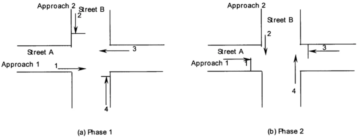
The National Electronic Manufacturers Association (NEMA) developed a functional standard in the traffic control field. NEMA controllers have similar functionality, which is widely used in the U.S. The controller operates based on phase diagrams that define the compatible phases and the order in which phases are displayed. An example of a simple four-phase diagram is show in Figure 2.1. The east-west movements are served first, with the left turns in Phase 1 and with through and right movements in Phase 2, followed by the left and through/right movements for the north-south street in Phases 3 and 4, respectively. Each phase has a logic specified for its green timing, which may be pre-timed or demand responsive. The phase order is specified using the "conflict clearance" condition. In this example, Phase 2 will wait for Phase 1, Phase 3 for Phase 2, and Phase 4 for Phase 3, and Phase 1 for Phase 4, thus defining the proper phase order.
1 2 3 4
Figure 2.1 Four-phase Controller Diagram
An eight-phase controller that is more flexible in the phase progress is commonly used. It supports fully actuated control. Figure 2.2 shows the typical phase diagram for such a controller. The eight-phase controller operates two four-phase rings simultaneously,
allowing the rings to advance independently. For example, the controller will start by displaying Phases 1 and 5 because neither of Phases 1 or 2 conflicts with Phases 5 or 6, and then each phase can advance to its following phase when it is ready. The phase pairs of 1 & 5, 1 & 6, 2 & 5, and 2 & 6 are compatible and thus can be active simultaneously. The barrier that separates the primary street and cross-street movements imposes a restriction on the independence of the rings. Because all movements on one side of the barrier conflict with all movements on the other side, the rings must advance simultaneously across the barrier to prevent conflicting movements from being active simultaneously.
Earrier
1 2 3 4
5 6 7 8
Figure 2.2 Eight-phase (dual-ring) Controller Diagram
Figure 2.3 shows the different phase sequences of the eight-phase controller. The phasing is similar to the four-phase controller with the addition of alternate transition phases where left and through movements may operate concurrently. Which transition phase used, if any, will depend on the ending times of Phases 1 and 5, determined either by preset timings or by vehicle actuations. Each phase has a preceding phase defined to specify the phase order. The barrier is modeled with the "complementary group" condition, which will hold a phase passively in green while another phase is still active. In the example above, Phases 2 and 6 are defined as complementary. This condition constrains their green intervals to end at the same time, assuring that the phase rings cross the barrier simultaneously. Phases 4 and 8 are similarly defined, modeling the return across the barrier to Phases 1 and 5.
2&5 4&7
I & 5 2& 6 3 & 7 4 & 8
1& 6 3& 8
Modem traffic-actuated controllers usually implement a dual-ring concurrent phasing in which each phase controls only one movement, but two phases are generally being displayed concurrently. The term, "phase group", is used in the analysis of intersection capacity, which is set of phases that are being displayed concurrently.
2.3.2 Timing Characteristics
In an actuated phase, there are three timing parameters: the minimum green interval, the unit extension, and the maximum green interval. These intervals are a function of the type and configuration of the detectors installed at the intersection. These three intervals are shown in Figure 2.4. This figure shows a case that the phase terminates before it reaches the maximum green period because there is no vehicular actuation in the last unit extension period.
Total green period
Minimum green Extension period
Unit extension (Passage time) Initial Interval
Actuations
Maximum green
Time
Detector actuation on a conflicting phase
Detector actuation on phase with right of way
E-1 Unexpired portion of unit extension
Figure 2.4 Actuated Phase Intervals
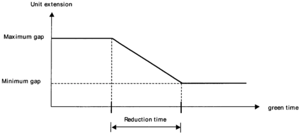
The unit extension is time by which a green phase could be increased during the
extendable portion after an actuation on that phase (Garber and Hoel, 1997). It depends on the average speed of the approaching vehicles and the distance between the detectors and the stop line. The unit extension can be determined by the following equation
eo= S (2-6)
where:
eo = unit extension (seconds);
v = average speed (mph);
S = distance between detectors and stop line (ft).
Initial interval is the first portion of the green phase that is adequate to allow vehicles
waiting between the stop line and the detector during the red phase to clear the intersection (Garber and Hoel, 1997). This time depends on the number of vehicles waiting, the average headway, and the starting delay. The initial interval can be obtained as
I= (hn + KI) (2-7)
where:
h = average headway (seconds);
n = number of vehicles between the detectors and the stop line;
K = starting delay (seconds).
Suitable values for h and K are 2 seconds and 3.5 seconds, respectively.
The minimum green interval is the shortest time that should be provide for a green
interval during any traffic phase. In basic design of actuated phase intervals, the minimum green interval equals the sum of the initial interval and the unit extension. In the advanced design of NEMA controller as shown in Figure 2.4 the minimum green interval may be less than the initial interval plus one unit extension.
The maximum green interval is the limit that a phase can hold green in the presence of
conflicting demand. Normal range of maximum green is between 30 and 60 seconds depending on traffic volumes (Kell and Fullerton, 1991). Webster's model for pretimed controllers can be used to compute the maximum green interval. The computed green intervals are multiplied by a factor ranging between 1.25 and 1.50 to obtain the maximum green (Kell and Fullerton, 1991). NEMA specifies that the maximum green time not begin timing until there is a serviceable conflicting call. Therefore, a phase may remain green for some time before a conflicting demand appears that starts timing the maximum green.
The logic of a typical semi-actuated control has the following features (Kell and Fullerton, 1991):
The green duration for the side street starts with a predetermined initial interval, which is followed automatically by one unit extension eo. If there is a side street vehicle actuating the detector during this unit extension, the green duration may be extended repeatedly in the same fashion until the maximum allowable green interval, is reached. If no single vehicle actuates the detector during a unit extension, the green duration will be terminated at the end of the unit extension.
According to this control logic, the average cycle lengths and cycle splits of a semi-actuated control are not affected by the traffic on the major street.
A fully actuated control does not distinguish between a major street and a side street. Every street is treated like a side street that is under a semi-actuated control. The control logic for each signal phase is the same as the one applicable to a side street under a semi-actuated control. Consequently, the resulting average cycle lengths and cycle splits depend not only on the signal timing plans but also on the traffic pattern in each phase. In density mode, the unit extension time can also be set to vary as a function of the elapsed green time, usually reducing the extension time as the maximum time is neared. A variable extension length is often used because a long extension time is desirable at the start of the phase to ensure that vehicles are cross the intersection, while a shorter extension is desired near the end of the phase so that the phase is not extended unnecessarily (McShane et al., 1990). A typical "gap-reduction" function is show in Figure 2.5. Unit extension Maximum gap Minimum gap
I
green time Reduction timeFigure 2.5 A Gap-reduction Function
Traffic-actuated controllers automatically determine cycle lengths and phase durations based on detection of traffic on the various approaches. The cycle lengths and green times are random variables, which depend on the real-time traffic demand. Therefore, the capacities of approaches to an intersection are random variables. A comprehensive review of the models estimating the timing plans and the approach capacities is presented in Section 2.5.
2.4 Adaptive Control
Adaptive control uses timing plans that are computed in real time, based on forecasts of traffic conditions. The detector observations are used as input into a prediction algorithm. This control is conceived as highly responsive with signal timing adjusted in small and frequent intervals. Examples of adaptive control systems are SCOOT (split, cycle and offset optimization technique) developed in the U.K., OPAC (Optimized Policies for Adaptive Control) developed in the U.S. and SCAT (Sydney Coordinated
Adaptive Traffic System) developed in Australia. We review the first two control systems in this section.
2.4.1 Traffic-Responsive System (SCOOT)
SCOOT is a traffic-responsive urban traffic control system for optimizing network traffic performance. The systems monitor traffic conditions in a network by some form of detection and react to the information received by implementing appropriate signal settings. The SCOOT system adapts itself to traffic patterns and responds to traffic demands as they occur. The more recent version of the SCOOT system operates by interpreting comprehensive detector information online and monitors traffic flows continuously from on-street detectors. It uses this information to recalculate its traffic predictions every few seconds and then makes systematic trial alterations to current signal settings. New plans are continuously evolved in SCOOT system, which is valuable in central areas where congestion is high and flow patterns are complex and variable.
Inductive-loop detectors measuring vehicle presence (occupancy) are placed at the upstream end of each link in the SCOOT network and transmit the occupancy data to the central computer. The cyclic flow profiles for each link reveal the variation in traffic demand during each cycle. The detectors measure the cyclic flow profiles that are used to optimize signal coordination and for measuring and/or predicting queues, stops and congestion on each link. They are used during offset optimization to ensure good signal coordination.
The optimization model determines the signal timings that minimize a performance index (PI) for each SCOOT region, based on a weighted sum of delays and stops. For each traffic flow pattern and link-node arrangement a PI is calculated as (McDonald and Hounsell, 1991)
PI = Wwd + KkiSJ (2-8)
where:
N= the number of links;
W= the overall cost per average passenger car unit (pcu) equivalent hour of delay; K = the overall cost per 100 pcu stops;
O,= the delay weighting on link i; d, =the delay on link i;
k= the stop weighting on link i; and Si= the number of stops on link i.
The weighting factors balance the relative importance of queues and stops. A tendency exists to favor somewhat longer cycle times by using a heavy weight for stops (Roberston, 1986).
A SCOOT controlled network is divided into a number of regions. The SCOOT optimizer updates the traffic signal plan on a cycle-by-cycle basis. In doing this, the optimizer uses the previous cycle's signal settings as a seed in the search for new timings and makes minor alterations to these seed signal settings. The changes to the signal settings are made based on a restricted search for a minimum PI in the immediate vicinity of the seed signal settings, rather than by an exhaustive search for a global minimum PI (Rakha, 1995). The SCOOT adjusts signal timings in frequent small increments to match the latest traffic situation. These models ensure that queues cannot exceed a maximum queue value for each link.
The cycle time optimizer estimates the optimal cycle time for the region. The intersections
in each region operate to their own common cycle time to ensure good signal coordination. For each region the model calculates the degree of saturation for all its nodes. It identifies the most critical node for each region and calculates the optimal cycle length which is used by all nodes. The cycle time is determined on the basis that the most heavily loaded intersection in the region should operate at a maximum degree of saturation of about 90%.
The split optimizer decides whether it will advance, postpone, or leave alone the green
times for each stage. It seeks to balance the degree of saturation on all approaches and to avoid blocking-back. The green split is determined by minimizing the maximum degree of saturation on the approaches to that intersection. The level of congestion can also be included as an optimization criterion. In this calculation, the current estimates by SCOOT of the queue lengths, of any congestion measured on the approaches to the intersection, and of the constraints imposed by minimum green time is taken into account. Typically the lower bound might be about 30 or 40 seconds. The upper bound is set to give maximum traffic capacity but without unduly long red times. A maximum cycle time of 90 to 120 seconds is typically used in SCOOT.
The offset optimizer determines every cycle whether or not to alter all scheduled stage
change times at an intersection. The sum of the PIs on all adjacent streets for the scheduled offset is compared with offsets that occur a few seconds earlier or later in determining the offset. The level of congestion can also be incorporated into the PI. The decisions of the offset optimizer are modified where congestion occurs; the purpose is to prevent queues of vehicles from growing to the point where upstream intersections are obstructed. Since congestion is more likely to occur on short sections of road, the offset optimizer acts to improve the coordination on the short streets by increasing queue on longer streets, which have space to store queues.
SCOOT is cycle-based and not fully reactive, and cannot respond to major discrete events appropriately in real time. It may also be slow in evolving with rapidly changing traffic demands, such as during the morning rush hour. It may therefore be providing slowly evolving "old" plans under such dynamic conditions. In addition, SCOOT is not efficient
algorithms for true real-time control that are compatible with a central control system. Further research on grouping signals into sub-areas may lead to new algorithms that are of sufficient generality and simplicity as to be attractive for on-line use. SCOOT has been developed for use when traffic demands are moderate to heavy. When traffic flows are low, it may not be necessary to run all the stages during every cycle time. However, SCOOT cannot skip traffic stages automatically.
2.4.2 Optimized Policies for Adaptive Control
OPAC is an on-line traffic signal timing optimization algorithm, which was developed as a distributed system for traffic signal control without requiring a fixed cycle time. Signal timings are calculated to directly minimize performance measures, such as vehicle delays and stops, and are constrained by minimum and maximum phase lengths. The first version of OPAC solved the traffic control problem, using a dynamic programming algorithm. Each time interval is designated as a stage, which is typically five seconds. A "rolling horizon" concept was applied to the OPAC algorithm in order to use real time flow data. The horizon is typically equal to the average cycle length during which the OPAC calculates its switching decisions. The modified version was a simplification of the algorithm using dynamic programming. This version was reorganized for implementation in real time in a control system.
OPAC was improved by incorporating a traffic prediction model that predicts the traffic pattern over the entire stage. The horizon consists of a head and a tail portion. In the head portion of the horizon, the algorithm has available real-time vehicle arrival information. In the tail portion, the flows are estimated from previous measurements (Gartner, 1991). The detectors are placed well upstream of the intersection in order to obtain actual arrival information over the head period. Delay is calculated based on particular phase change decisions.
In OPAC, stops were included in the objective function, which is typically a linear combination of delays and stops, with the weight of stops relative to delay being one. In reality, this weight favors delay. At each individual intersection, phase plans are generated for future implementation based on current traffic conditions (i.e., current queues and expected arrivals) so as to minimize the objective function over a "decision horizon." A phase plan is a sequential list of future switch points with each switch point representing the start of a certain phase at a specific time in the future. Traffic conditions are continuously monitored based upon vehicle detector and phase change information. The decision horizon typically ranges from less than thirty seconds to greater than two minutes in length. Phase plans are continually regenerated for the entire decision horizon but implemented only for the first three to five seconds. This "rolling-horizon process" allows signal timings to be constantly adapted to new traffic condition.
The optimization process is decomposed into N stages. The total number of stages N corresponds to the horizon length. At stage i, the input state vector is I, the arrivals vector is Ai, the output state vector is Oi, and the economic return output is ri. A set of transformation functions is (Gartner, 1982):
01 = T (I, Ai, ri) (2-9)
ri = Ri (I, A,, r,) (2-10)
The state of the intersection is characterized by the state of the signal and by the queue length on each of the approaches. The input decision variable indicates whether the signal is to be switched at this stage or to remain in its present state. The return output is the intersection's performance index. The optimization process minimizes the total performance index.
The dynamic programming optimization is carried out in backwards order, i.e., starting from the last stage and back-tracking to the first, at which time an optimal switching policy for the entire time horizon can be determined (Gartner, 1982). The recursive
optimization function is given by the following equation,
f*
(I,) = min{Rj (Ii, A , x) +f*j
(I , A, ,x1)}
(2-11)where the return at stage i is the queuing delay incurred at this stage:
RIA,,x)=
±I"
- D7 )=Q
(2-12)a a
where:
a = approach designation, by direction, a = N, S, E, W;
A," = number of arrivals during stage i;
Da = number of departures (discharges) during stage i;
Q7
= the queue length on the approach at the beginning of stage i.The departure rate is a function of the state and decision variables (Gartner, 1982):
0 if Sa =1
D={Q+A if S" =0,Q+A 2 (2-13)
2 if S" =0,Q+A>2
where Sa is the signal status for approach a, defined as follows:
0 if green S" =
.
if red
When the optimization is completed at stage i = 1
N N
which is the minimized total delay over the horizon for a given input state I,. Since the initial conditions at stage 1 are specified, the optimal policy is retraced by taking a forward pass through the stored tables of X (Ii). The policy consists of the optimal sequence of switching decisions { X*, i = 1, ... , N} at all stages of the optimization
process.
The OPAC strategy carries out sophisticated optimization in real time and adapts to varying traffic conditions. Field tests have shown that OPAC can provide significant benefits over well-timed actuated controllers. Because OPAC is not a traffic-driven controller, it forms a building block for a distributed intelligent traffic control system. Unlike conventional actuated control logic, the OPAC system can communicate with neighboring controllers so as to form a flexible coordinated traffic control system. OPAC uses the same performance measure as objective function for both off-peak traffic and peak traffic. A field test shows that when the observed volumes were extremely low the improvements were modest, because stops were not an OPAC measure of effectiveness in the first version of the system. OPAC adds to the optimization objective function a penalty, which is composed of the weighted sum of final queues on each approach. The penalty is added to minimize the final queues so that only minimal queues are transferred to the succeeding stage. At high level of volumes queues on some approaches may spread to the upstream intersection because OPAC system does not impose constraints on queues on approaches to an intersection. The unconstrained queues will reduce the capacity of the neighboring intersections.
2.5 Methods for Estimating the Capacity of Traffic-Actuated Intersections
The intersection capacity is a function of flow rates on approaches to an intersection for use in dynamic traffic assignment. The intersection capacity is represented by the capacities of approaches to the intersection. In general, the approach capacity is a function of the green time allocated to this approach, the cycle length of the intersection, the saturation flow rate of the approach, and the characteristics of the approaching flows. The capacity of approach a to the intersection can be determined as:
Ca = S(G /C)a (2-15)
where:
Ca= the capacity of approach a, in vph;
Sa= the saturation flow rate for approach a, in vphg;
C = the cycle length of the intersection, in seconds; and
Ga = effective green time for approach a, in seconds.
We review three models that estimate the green times and cycle lengths at an intersection with actuated control in this section.
2.5.1 Allsop's Method
Allsop (1972) formulated the capacity of a signalized intersection as a linear programming problem. The model can be used to design signal-timing plans by maximizing the capacity of approaches to an intersection and to determine approach capacities of the intersection as well. His results apply to both intersections in linked systems where traffic arrives mainly in platoons and isolated intersections where the traffic arrives at random because no assumption about the arrivals of traffic is made. A part of the signal cycle in which one particular set of approaches has right of way is called a stage. At stage
j,
the proportion A of the cycle that is effectively green forapproachj is given by m
Ai =I aUAJ) (2-16)
where:
= the proportion of cycle that is effectively green for stage i (i = 1, 2, ..., Im);
a =1 if approachj has right of way in stage i ( i= 1, 2, ... ,n), and 0 if not; and a0, = proportion of total lost time that is effectively green for approachj (i = 1, 2,
..., n).
The arrival rates on all approaches are multiplied by t. The queues and delays on all approaches will be acceptable if Ai> pbi (=1, 2, ... , n), i.e., if
aui)- pbj 0 (j=1, 2, ... , n) (approach capacity constraints) (2-17)
where:
bj= the smallest acceptable value of Aj when the arrival rate is q1;
s1 = the saturation flow;
p1= adjustment factor of the sj, the value is chosen by the engineer; and
bj = q/pjsj. (2-18)
In addition, the signal settings must satisfy the following constraints,
Ai - kiAO 0 (i=1, 2, ..., m) (minimum green constraints); (2-19)
AO
k
ko; (2-20)and
where:
ki= giM/L; (2-22)
ko= L/C; (2-23)
where:
gim = minimum green time for stage i (i = 1, 2, ... , m);
C = the maximum of specified cycle time; and
ko = the proportion of the cycle taken up by the lost time, L/C.
P4*1], (u* = A1/bj) is the largest value of u such that the delays and queues are acceptable.
Then uj*qj is the practical capacity of approach
j
when the proportion of the cycle of effective green for this approach is Aj. p* can be solved as a linear programming problem:Maximize p* Subject to:
Equations (2-17), (2-19), (2-20), and (2-21).
Let pj be the maximum degree of saturation that is acceptable on approach j. The approach capacity is defined as
c = p s1AC forj = ,...,n. (2-24)
Allsop's method (1972) does not provide a closed form expression of p*. In order to get optimal u, one needs to solve the above linear programming problem. His formulation is appropriate for solving the signal design problem. However, Allsop's method is not applicable to estimation of the approach capacities in DTA since a linear program has to be solved for each intersection and time interval.
2.5.2 Daganzo's Method
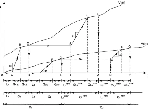
Daganzo (2000) discussed an actuated control strategy that operates with cycles and phases close to the minimum while avoiding overflows. With this strategy traffic delay would be reduced by a factor of two, comparing with the pre-timed timing plan from Webster's model (Daganzo, 2000). The control strategy is: The actuated systems end the green phase on each approach as soon as its queue dissipates. Figure 2.6 illustrates this strategy by a simple intersection with two phases. The figure depicts two cumulative (virtual) arrival curves, V1(t) and V2(t), starting at an instant (t = 0) when the queue at Approach 2 has vanished and the queue of Approach 1 is QI(O) >0. The saturation flows and the lost times for both approaches (se, Li) are known. The departure curves are constructed for any pair of V(t)'s. On the arrival and departure curves, arrowheads indicate the order in which points along the departure curves are obtained.
V1(t) N B H V2(t) Q1(0) si E 0 A CD F G J K t Li Gi L2 G2 Li" Gi n
Figure 2.6 The Actuated Traffic Signal Strategy under which Green Phases Terminate as soon as their Queues Vanish
Daganzo (2000) derived the cycle length equation for this actuated control strategy. The
following is the summary of the result. The average duration of a green phase for approach i, is G.. Each cycle has a total lost time L = L1+L2. q, denotes average flow in
an interval. The Cycle length is estimated as,
C=L 1-1yi (2-25)
where y, = qi I s.
The effective green ratio can be determined as,
Ai = Gi/ C = y, (i = 1,2). (2-26)
The above-mentioned actuated strategy is suitable for isolated intersections of major streets with under-saturated conditions. If traffic becomes over-saturated for an extended period, the strategy does not proactively allocate more green to the approach with the highest flow. Therefore, a long queue may be built up on the main street. In reality, the actuated signals do not work in the way as suggested by Daganzo. For instance, in the simple example illustrated in Figure 2.6, the Phase 1 terminates when the queue on Approach 1 dissipates. In practice, Approach 1 retains green time for an extended period until there is demand from Approach 2 or interarrival headway of traffic on Approach 1 is longer than the unit extension. Therefore, neither Equation (2-26) nor Equation (2-25) is appropriate for estimating green times of actuated control.
The above model also underestimates the average cycle length because it was essentially the cycle of an actuated signal for the queue to dissipate. If there is no recall from other phases, the green time on the last phase will extend to the maximum green time. The
actuated signals usually operate at cycle length between the minimum length and the maximum length. However, Daganzo's method can be used to estimate the queue service times of an actuated intersection, which is used to estimate the capacity of approaches to actuated intersection.
2.5.3 Highway Capacity Manual Methodology
Pretimed Control
Chapter 16 of the HCM 2000 describes a model for estimating the capacity and signal timing plans at a signalized intersection as a function of the traffic characteristics. The HCM suggests that the average cycle length and phase times may be approximated by assuming that the controller is effective in its objective of keeping the critical approaches nearly saturated. The cycle length is given by the following equation:
C =LXC /[Xc -( I(v/s)c (2-27 )
where:
C= cycle length, in sec;
L = lost time per cycle, in sec;
(v/s)ci = flow ratios for critical lane group i; and
X = critical ratio of volume to capacity for the intersection.
The effective green time for a particular phase, Gi, is estimated with the following equation
vC v C
G- i (2-28)
where:
Xi=ratio of volume to capacity for lane group i;
vi= demand flow rate for lane group i, vph;
s= saturation flow rate for lane group i, vphg; and Gi= effective green time for lane group i, sec.
The average cycle length can be estimated using a user-specified X. The capacity of a lane group can be calculated by Equation (2-15) after the cycle length of the intersection and green time for lane group i are determined. This procedure is appropriate for estimating the lane group capacities of intersections with pretimed control.
Traffic-Actuated Control
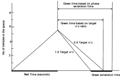
The HCM 2000 describes a method for estimating the capacities of intersections with actuated control, which is sensitive to variations in design parameters. The models were developed based on the concept of queue accumulation polygon (QAP) which plots the
number of vehicles queued at the stop line over the cycle. Figure 2.7 depicts the QAP for a simple protected movement where the accumulation takes place on the left side of the triangle and the discharge takes place on the right side of the triangle. The duration of a green interval is determined by the length of the previous red interval and the arrival rates. The average green time of a phase is estimated as the sum of the queue service time and the phase extension period as shown in Figure 2.7.
8 E 0 0 z 6 4 2
Green time based on phase extension time
Red Time (seconds) Green extension time
Figure 2.7 Queue Accumulation Polygon Illustrating Green Time Computation
The queue service time, Gq, is given by
G = fq qr (2-29)
q q(s - q,)
where:
q,., q,= red arrival rate (veh/sec) and green arrival rate (veh/sec), respectively;
r = effective red time (sec);
s = saturation flow rate (veh/sec);
fq =1.08 -0.1(G/Gmax) 2 (2-30)
where:
G = the actual green (not including yellow time) (sec); and
Gmx= maximum green (sec).
The queue calibration factor, fq, accounts for randomness in arrivals in determining the average queue service time.
Green time based on target
v/ c ratio
0.9 Target v/ c
The green extension period, Ge, is estimated by an analytical model, which was
developed by Lin (1982) and improved by Akcelik (1994). Ge is estimated assuming that vehicle arrival according to the bunched exponential arrival headway distribution:
O(e0 +to -A)
Ge = - - (2-31)
(IJ 0
where:
q = the total arrival flow (veh/sec) for all lanes that actuate the phase under
consideration;
eo= the unit extension time setting (sec);
to= the duration during which the detector is occupied by a passing vehicle (sec),
to =0.68(Ld +L)/SA (2-32)
where:
L,= vehicle length, assumed to be 18 ft; Ld= detector length (ft);
SA = vehicle approach speed (mi/hr);
A = minimum arrival (intra-bunch) headway (seconds); rp= proportion of free (unbunched) vehicles;
0 = a parameter calculated as:
0 = (p (2-33)
1- Aq
The proportion of free vehicles in the traffic stream, p, is determined by the following relationship originally proposed by Brilton (1988)
(o = e--bq (2-34)
where b is a bunching factor. HCM recommends parameter values as follows:
Single-lane case: A = 1.5 s and b = 0.6
Multi-lane case (2 lanes): A = 0.5 s and b = 0.5 Multi-lane case (3 or more lanes): A = 0.5 s and b = 0.8
Green times are subject to the constraints of minimum and maximum green times, which are controller parameters. The capacity of lane groups of an intersection can be estimated by Equation (2-15) after the cycle length of the intersection and the green times are determined.
The method does not directly determine an average cycle length and green times, since the green time required for each phase depends on the green times required by the other phases. Thus, a circular dependency exists which should be solved iteratively. HCM recommends an iterative procedure to compute the queue service time and green extension period as follows:
The logical starting point for the iterative process involves the minimum times specified for each phase. If these times turn out to be adequate for all phases, the cycle length will simply be the sum of the minimum phase times for the critical phases. If a particular phase demands more than its minimum time, more time should be given to that phase. Thus, a longer red time must be imposed on all of the other phases. This, in turn, will increase the green time required for the subject phase.
Although the iterative procedure applicable to off-line capacity estimation, it is not applicable to the dynamic traffic assignment because of the real time nature of many applications. In addition to increasing the run time of DTA, the procedure usually does not converge to the actual green times. Therefore, a model that does not require iterative computation needs to be developed.
The following numerical example, which is used in the HCM 2000, demonstrates the estimation problem of the HCM method. Consider the intersection of two streets with a single lane in each direction. Each approach has identical characteristics, and carries 675
vehicles per hour with no left or right turns. The intersection is controlled by a two-phase actuated signal with one phase for the east-west movement and the other for north-south movement. The average headway is 2.0 seconds per vehicle and the lost time per phase is 3.0 seconds. The actuated controller settings are:
Initial interval: 10 seconds Unit extension: 3 seconds Maximum green: 46 seconds Inter-green: 4 seconds
Using the HCM approach, the estimated value of green extension for each approach is 7 seconds since the approach flow rates are the same. The solution of the queue service time, a part of effective green time, is 39 seconds for each phase. The estimated cycle length is 2x (39 + 7) + 2x3 + 4 = 102 seconds assuming that the total all-red time is 4 seconds. This result is slightly lower than the cycle length determined by Webster's model (For the demands at the intersection, the cycle length determined by Webster's model is 112 seconds).
In this example, the minimum phase time is, initial interval + unit extension + inter-green, which is 10 + 3 + 4 = 17 seconds for both phases. If a particular phase demands more than its minimum time, then more time must be given to that phase. Thus, a longer red time is imposed on all of the other phases. This, in turn, will increase the green time required for the subject phase. Since there is not any objective function and no
constraints in the iterative procedure, the cycle length converges at the one, which is longer than the actual cycle length.
2.5.4 Traffic Control System Handbook
The Traffic Control System (TCS) Handbook (1996) provides a model for determining cycle length of actuated intersection, which is derived from Webster's model (1958), as follows,
C 13L (2-35)
1= - yi
where yi is the maximum ratio of flow rates to the saturation flow rates for approaches sharing the phase i and n is the number of phases. The cycle length estimated by this model is essentially 1.3 times the time interval for queues to dissipate. It cannot be justified that the actual length of a phase is 1.3 times the time for the queue to dissipate. In addition, the TSC model does not appropriately account for the mechanism of actuated control. Therefore, this model is not appropriate for capacity estimation for actuated intersections.