HAL Id: hal-03155833
https://hal.archives-ouvertes.fr/hal-03155833
Submitted on 2 Mar 2021
HAL is a multi-disciplinary open access archive for the deposit and dissemination of sci-entific research documents, whether they are pub-lished or not. The documents may come from teaching and research institutions in France or abroad, or from public or private research centers.
L’archive ouverte pluridisciplinaire HAL, est destinée au dépôt et à la diffusion de documents scientifiques de niveau recherche, publiés ou non, émanant des établissements d’enseignement et de recherche français ou étrangers, des laboratoires publics ou privés.
Numerical and experimental investigation on the
realization of target flow distribution among parallel
mini-channels
Min Wei, Guillaume Boutin, Yilin Fan, Lingai Luo
To cite this version:
Min Wei, Guillaume Boutin, Yilin Fan, Lingai Luo. Numerical and experimental investigation on the realization of target flow distribution among parallel mini-channels. Chemical Engineering Research and Design, Elsevier, 2016, 113, pp.74-84. �10.1016/j.cherd.2016.06.026�. �hal-03155833�
1
Numerical and experimental investigation on the realization of target flow
1
distribution among parallel mini-channels
2
Min WEIa, Guillaume BOUTINa, Yilin FANa, Lingai LUOa* 3
a
Laboratoire de Thermocinétique de Nantes, UMR CNRS 6607, Polytech' Nantes –
4
Université de Nantes, La Chantrerie, Rue Christian Pauc, BP 50609, 44306 Nantes Cedex 03,
5 France 6 7 Abstract 8
Fluid flow maldistribution is considered as one of the main causes of performance 9
deterioration in various energy and process systems, especially when parallel micro- or 10
mini-channel fluidic networks are involved. For a specific purpose, the optimal flow 11
distribution is not necessarily uniform. However, specific non-uniform distributions are 12
somewhat more difficult to achieve than uniform ones. The insertion of a geometrically 13
optimized baffle has been numerically confirmed as an effective solution to this issue, but 14
experimental validation is still lacking which is indispensable for bridging the gap between 15
theory and practice. 16
This paper presents a numerical and experimental investigation on the realization of 17
target flow distribution among parallel mini-channels, using the optimized baffle insertion 18
method. A 15-channel fluidic network integrated with the distributor and the collector is 19
fabricated and tested. Various perforated baffles are optimized and fabricated corresponding 20
to different target distributions (uniform, ascending and descending). PIV technique is used 21
for the flow distribution measurement while CFD simulations are also performed for 22
comparison. CFD results and PIV data show that different target distributions could be 23
successfully achieved by the optimized baffle insertion method. The robustness of the 24
optimized baffle for uniform distribution is also evaluated and discussed to provide some 25
guidelines for future applications. 26
27
Keywords: Parallel mini-channels; Flow distribution; PIV; CFD; Perforated baffle
28
29
30
* Corresponding author. Tel.: +33 240683167; Fax: +33 240683141. E-mail address: lingai.luo@univ-nantes.fr *Manuscript
2
1 Introduction
1
Fluid flow maldistribution is considered as one of the main causes of performance 2
deterioration in various energy and process systems, such as heat exchangers (e.g., Lalot et al., 3
1999; Fan et al., 2008; Tarlet et al., 2014), fluidized beds (e.g., Ouyang et al., 1995; Ong et al., 4
2009), chemical reactors (e.g., Saber et al., 2010; Guo et al., 2013, 2014), solar receivers (e.g., 5
Fan and Furbo, 2008; Salomé et al., 2013; Wei et al., 2015a) and heat sinks for cooling (e.g., 6
Sehgal et al., 2011; Siva et al., 2014). Nowadays, increasing attention has been devoted to 7
miniaturized fluidic networks in which the flow distribution among parallel micro- or 8
mini-channels should be properly controlled for enhanced heat and mass transfer and safety 9
reasons (Luo, 2013). 10
In the majority of the existing literature, flow maldistribution is synonymous with 11
“non-uniform flow distribution”, implying that uniform shape is assumed, or considered to be 12
the optimal distribution among parallel channels. Various methods have been proposed to 13
improve the fluid flow uniformity, as summarized in Rebrov et al. (2011) and Luo et al. 14
(2015). Through continuous efforts of academic or industrial researches, uniform fluid flow 15
distribution has become a more or less realistic goal. However, recent studies (e.g., Milman et 16
al., 2012; Boerema et al., 2013; Wei et al., 2015a) clearly show that the optimal flow 17
distribution may not necessarily be uniform, but usually non-uniform corresponding to a 18
defined objective function and constraints for optimization. The extension of the term “flow 19
maldistribution” from “non-uniform distribution” to “non-optimal distribution” (Wet et al., 20
2015b) raises higher requirements for the design and optimization of flow distribution 21
devices which are beyond the capabilities of conventional empirical propositions or 22
trial-and-error attempts. 23
In our previous study (Wei et al., 2015b), a Computational Fluid Dynamics (CFD)-based 24
evolutionary algorithm has been developed with the aim of realizing the target flow 25
distribution among parallel channels. The basic idea is to install a thin perforated baffle at the 26
distributing manifold and to optimize the size and distribution of orifices, in order to reach 27
the target flow-rate in every downstream channel. The effectiveness of the proposed 28
evolutionary algorithm has been tested by several 2D examples with different fluidic network 29
geometries (axisymmetric or nonaxisymmetric) and different target curves (uniform, 30
ascending, descending, or step-like). Numerical results show that the optimized flow 31
distributions reached are in good agreement with the target curves. As the first attempt on the 32
realization of target flow distribution, the optimized baffle insertion method has been 33
numerically confirmed as a practical solution to this issue. However, the proposed method 34
depends strongly on the accurate simulations of fluid flow so that experimental validation of 35
CFD models as well as the proposed algorithm is indispensable for bridging the gap between 36
theory and practice. This involves the simulation and optimization of 3D objects, their 37
fabrication and experimental characterizations which are still lacking. 38
3
The current study aims at presenting an experimental validation of the optimized baffle 1
insertion method for the realization of target flow distribution among parallel mini-channels. 2
For this purpose, different perforated baffles are designed, optimized, fabricated and installed 3
in a 15-channel fluidic network to test their capability of realizing different target 4
distributions (uniform or non-uniform). In parallel, 3D CFD simulations are also performed, 5
providing a comparison with the experimental results. 6
The experimental technique used in this study is based on flow visualization using 7
Particle Image Velocimetry (PIV) technique. Through recording the movement of seeding 8
particles illuminated by the pulsed sheet laser, the fluid flow velocity profiles can be obtained. 9
Compared to conventional flow-rate measurement techniques, such as Hot Wire Anemometry 10
(HWA) or Pitot tube, PIV as a non-intrusive method will not disturb the fluid flow 11
streamlines. Another advantage of PIV is the whole-field (or multiple points) measurement 12
which is unique compared with other non-intrusive single point measurement techniques, 13
such as Laser-Doppler Velocimetry (LDV) and Doppler Ultrasonic Velocimetry (DUV). A lot 14
of successful applications of PIV for fluid flow measurement have been reported in the 15
literature, including single phase (air or water) (e.g., Meinhart et al., 1999; Wen et al., 2006) 16
or multi-phase flow (e.g., Kiger and Pan, 2000; Lindken and Merzkirch, 2002), laminar or 17
turbulent flow (e.g., Sheng et al., 2000; Westerweel et al., 2013) and coupled thermo-fluid 18
characteristics (e.g., Carlomagno and Ianiro, 2014). Therefore, it is considered as a reliable 19
and accurate technique for flow-rate measurement. 20
In the rest of this paper, we shall first introduce the 15-channel fluidic network device 21
fabricated for study and optimized perforated baffles used for different operation conditions. 22
Then the experimental set-up and measuring procedure will be presented, as well as the 23
numerical parameters for CFD simulations. After, the numerical and experimental results of 24
several cases for different target distribution curves will be presented, compared and 25
discussed. The effective range of the optimized baffle when the working condition varies 26
from the design value will also be evaluated and discussed to provide some guidelines for 27
future applications. Finally, main conclusions and perspectives will be summarized. 28
2. Fluidic network device and optimized baffles
29
In this section, the 15-channel fluidic network with the distributor and the collector will 30
be briefly introduced. The target distribution curves and optimized baffles will be presented 31
as well. 32
2.1 15-channel device
33
A mini-channel fluidic network consisting of 15 parallel channels, a distributor and a 34
collector is used for study, as shown in Fig. 1. The overall dimension of fluidic network is 35
242 mm in length and 90 mm in width. For the convenience of fabrication, the entire fluidic 36
network has the identical depth (e=2 mm). The inlet and outlet tubes located in diagonal 37
position have the same width of 5 mm, but different lengths (50 mm for inlet tube and 100 38
4
mm for outlet tube). The length of the distributing manifold is 13 mm and the width is 90 mm. 1
In the distributing manifold, a groove with the thickness of 1 mm and the width of 96 mm is 2
reserved for the installation of a perforated baffle. Identical dimensions are used for the 3
collecting manifold (length of 13 mm and width of 90 mm) but without baffle groove. 4
5
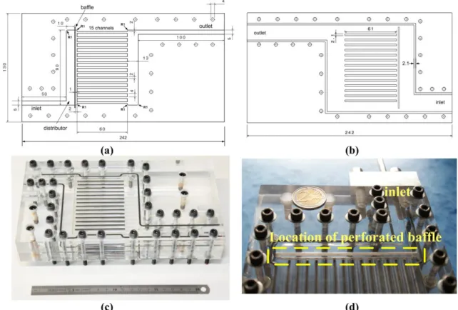
Figure 1: Geometry and dimensions of 15-channel fluidic network (unit: mm): (a) Parallelepiped A; (b) Parallelepiped B; 6
(c) Photo view after assembling; (d) Zoom on the inlet distributor and the location of the perforated baffle. Adapted from 7
Boutin et al. (2016). 8
There are fifteen parallel straight channels having identical width of 2 mm, length of 60 9
mm and depth of 2 mm. They are evenly spaced at 4 mm between the axis of one channel and 10
another. For the convenience of description, they are indexed by k from 1 to M from the inlet 11
side to the outlet side. The mass flow-rate in kth channel is notated as mk and the flow-rate 12
ratio is introduced for each channel as follows: 13 k k m m (1) 14
where m is the average mass flow-rate among 15 channels given by:
15 1 M k k m m M
(2) 16Note that it is a real 3D object with all parallel channels located in the same plane, suitable 17
for experimental tests of fluid flow distribution properties using visualization technique. 18
5
The device was fabricated in the laboratory LTN, France by digitally-assisted carving the 1
network on the surface of a PMMA rectangular parallelepiped (A), as shown in Fig. 1(a). Six 2
edge fillets (noted by R1 in Fig. 1(a)) having the same radius of 1 mm can be observed at 3
different corners of the fluidic network due to fabrication process. Another PMMA 4
rectangular parallelepiped (B) was also carved to form the enclosed fluidic network, as shown 5
in Fig. 1(b). Note that the depths of the groove reserved for the baffle are 6 mm in rectangular 6
parallelepiped A, and 4 mm in rectangular parallelepiped B to form the effective area of the 7
baffle (the area that may be touched or passed through by the fluid flow). A number of 8
grooves were reserved around the network or between neighboring parallel channels, and 9
filled with rubble strips to prevent the water leakage. Moreover, 29 bolts were used for 10
further sealing. The photo view of the 15-channel device after assembling is shown in Fig. 11
1(c) and the location of baffle is indicated in Fig. 1(d). 12
2.2 Target distribution curves and optimized baffles
13
To validate the effectiveness of the optimized baffle insertion method, different target 14
distribution curves are proposed to be realized, including a uniform curve, an ascending curve 15
and a descending curve. The geometric dimensions of the optimized baffles are obtained 16
accordingly using the CFD-based evolutionary algorithm developed in Wei et al. (2015b). 17
The thickness of the perforated baffle is 1 mm and the distance between the middle of the 18
baffle and the inlets of parallel channels is 2.5 mm. For the convenience of installation, the 19
baffle has a width of 96 mm and a height of 10 mm (as well as the groove for baffle), which 20
is a bit larger than the cross-section of inlet distributing manifold. Likewise, the height of 21
orifices is 3 mm, which is also larger than the thickness of the fluidic network (e=2 mm). 22
However, the effective area of baffle is kept at 90 mm × 2 mm. 30 orifices are distributed 23
equally on the effective area of baffle, with an identical spacing of 3 mm. For the 24
convenience of description, they are indexed from 1 to 30 from the inlet side to the outlet side. 25
For the initial uniform baffle subject to optimization (shown in Fig. 2), the orifices have 26
identical width of 0.6 mm, the global porosity thus being 20%. Since the thickness of the 27
entire network is fixed at 2 mm, the only variable for optimization is the width of orifice. 28
Note that some of the parameters used here are determined or selected based on the 29
parametric study presented in Luo et al. (2015) and Wei et al. (2015b). 30
31
Figure 2: Geometry and dimensions of the uniform baffle with identical width of orifices (unit: mm). 32
6
In this study, four perforated baffles are optimized under two different inlet total fluid 1
flow-rate conditions, i.e. high inlet flow-rate (Qin=1.8 L·min-1) and low inlet flow-rate 2
(Qin=0.18 L·min-1), for representing both the turbulent and laminar flow patterns. The 3
corresponding Re numbers in the inlet tube are 8500 and 850, respectively. The mean Re 4
numbers in the parallel channels (Rech) are 1000 for Qin=1.8 L·min-1 and 100 for Qin=0.18 5
L·min-1. The corresponding inlet flow-rate under which the perforated baffle is optimized is 6
named as the baffle’s design flow-rate. Baffles 1 and 2 are used for realizing uniform flow 7
distribution among 15 parallel channels respectively under low or high inlet flow-rate 8
condition (Qin=1.8 L·min-1; mean Rech=1000). Baffles 3 and 4 are optimized for respectively 9
achieving ascending or descending flow distribution under low inlet flow-rate (Qin=0.18 10
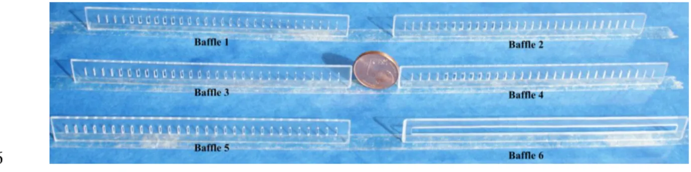
L·min-1; mean Rech=100). Baffle 5 is the uniform initial baffle with identical width of orifices 11
whereas Baffle 6 is named as "empty baffle" for representing the configuration of distributing 12
manifold without baffle insertion. The baffle number, the corresponding target curve, the 13
design inlet flow-rate and detailed dimensions of the orifices are summarized in Table 1 and 14
Fig. 3. Note that mk is the target value of mass flow-rate in kth channel. 15
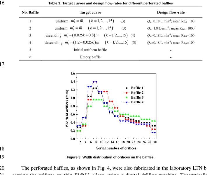
Table 1: Target curves and design flow-rates for different perforated baffles 16
No. Baffle Target curve Design flow-rate
1 uniform mk m k1, 2,...,15 (3) Qin=0.18 L·min-1; mean Rech=100
2 uniform mk m k1, 2,...,15 (3) Qin=1.8 L·min-1; mean Rech=1000
3 ascending m k 0.025k0.8m k1, 2,...,15 (4) Qin=0.18 L·min-1; mean Rech=100
4 descending m k 1.2 0.025 k m k1, 2,...,15 (5) Qin=0.18 L·min-1; mean Rech=100
5 Initial uniform baffle
-6 Empty baffle
-17
18
Figure 3: Width distribution of orifices on the baffles. 19
The perforated baffles, as shown in Fig. 4, were also fabricated in the laboratory LTN by 20
carving the orifices on thin PMMA slices, using a digital drilling machine. Theoretically, 21
more precise optimization results lead to better approaching of target curves, but also set 22
7
higher requirements on computational abilities and fabrication precisions. For this study, the 1
in-house fabrication tolerance is 0.01 mm and the minimum width of orifice is 0.16 mm, 2
implying a possible deviation between the numerically optimized distribution and the target 3
curve. To minimize this intrinsic maldistribution, more precise fabrication technologies 4
should be introduced, with smaller fabrication tolerances. 5
6
Figure 4: Photography of baffles used in this study. 7
The degree of closeness between the target curve and the optimized flow distribution 8
curve obtained by CFD-based evolutionary algorithm or by PIV measurement is quantified 9
globally by the maldistribution factor (MF) and locally by the maximum deviation 10 max defined as follows: 11 2 1 1 MF 1 M k k k m m M m
(6) 12 max max 1, 2,...,15 100% k k k m m k m (7) 133 Experimental setup and CFD simulation parameters
14
3.1 Experimental setup
15
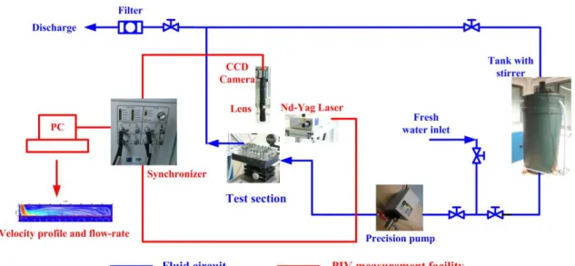
Figure 5 shows a schematic diagram of the experimental set-up built in the laboratory 16
LTN. It is composed of fluid circuit and PIV measurement facility. Pure water was used in 17
this study as the working fluid. In the fluid circuit, water was pumped from a 300 L water 18
tank, then passed through the test section (15-channel fluidic network), and finally returned 19
back to the water tank to form a closed loop. A precision pump (VWR, REGLO-Z, 20
instrumental error less than 0.1%) was installed in the circuit with a measurement range of 21
32-3200 mL·min-1 and the output mass flow-rate was controlled directly based on its own 22
readings. Fresh water was introduced to clean the 15-channel device after each series of tests 23
and a filter was used to avoid the discharge of sewage. 24
8
1
Figure 5: Schematic diagram of the experimental setup built for this study. 2
3
Standard 2D-2C PIV facility used in this study consists of illumination unit, image record 4
unit, synchronous controlling unit and data processing unit. The light source used was 5
Nd-Yag laser (Litron Incorporation, DualPower 65-15 DANTEC laser). The pulse energy was 6
65 mJ with the duration of 4 ns. The light wavelength was 532 nm and the diameter of light 7
beam was 6.5 mm. The pulse frequency is 5 Hz, indicating that the fluid flow was recorded 8
five times per second. The light scattered from the particles was collected by a CCD camera 9
(DANTEC, FlowSense) with 2048×2048 pixels. An additional macro LAVISION lens was 10
used to yield a magnification of about 230 pixel·mm-1, corresponding to the view field of 11
about 8.9 mm×8.9 mm. A synchronizer (DANTEC, 80N77) was used to guarantee that the 12
laser and the CCD camera work synchronously. A commercial software FlowManager (v3.41) 13
was used to control the PIV system and to process the data by 2-frame cross-correlation and 14
Fast Fourier Transforms (FFTs). In the current study, the size of the PIV interrogation 15
window was fixed at 16×16 pixels considering a compromise between the measurement 16
accuracy and the computational time. The spatial resolution of PIV for this study is about 17
0.19 mm, determined by 2.8 times of the size of interrogation window (Foucaut et al., 2004). 18
Polyamid Seeding Particles (PSP-5) supplied by DANTEC Company were used as seeding in 19
our study with good chemical stability and environmental friendliness. The particle density is 20
1030 kg·m-3 and the diameter of particles ranges from 1 µm to 10 µm with the average of 5 21
µm. 22
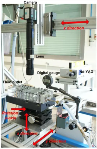
Figure 6 shows the workbench specially designed and built which permits the subtle 23
movements of the test-section. The camera can be moved in x direction whereas the platform 24
to fix the test-section is moveable in y and z directions. The movements in x and y directions 25
were realized using steel orbits while the movement of the platform along z direction was 26
realized using a precise lift and a digital gauge with an accuracy of 0.01 mm. The focus of the 27
lens must be adjusted for each vertical plane due to different scattered light optical paths, 28
leading to different magnification ratios which must be taken into account in the 29
9
post-processing. The platform can also be rotated around z-axis to ensure a fine overlap 1
between the walls of channels and the boundaries of the PIV interrogation windows. 2
Figure 6: Experimental workbench for subtle movements of the test-section. 3
3.2 Measurement procedure and uncertainty
4
To obtain the flow distribution properties among parallel channels, the flow-rate in every 5
individual channel should be measured when the total inlet flow-rate is stable. To do that, the 6
cross-section of each channel was divided into 9 planes along z direction for measuring the 7
velocity profiles using 2D-2C PIV technique, with a stepping distance of 0.25 mm. It should 8
be noted that the laser source was fixed so that the device should be moved vertically along z 9
direction for different measuring planes, using the adjustable workbench described above. 10
Due to the limitation of the test view of PIV, at most two channels can be measured together 11
each time. For a total of 15 channels, the fluidic network should be moved along y direction 12
and then eight successive measurements should be repetitively performed. 13
In our pre-test, two numbers of instantaneous frames, 200 and 375, were used for each 14
plane to test the image independence. The maximum deviation is less than 0.1% (Boutin et al., 15
2016). Therefore, 200 pairs of frames for each plane were enough to save the experiment and 16
post-processing time. In order to analyze the uncertainty of the 2D-2C PIV technique, the 17
results of total mass flow-rate obtained by PIV in this study are compared to the display of 18
high precise pump. The maximum possible deviation is 5.1% which will be indicated as the 19
10
error bar for PIV results in the following figures, implying that the PIV technique is relatively 1
accurate for flow-rate distribution measurements among parallel channels. More details on 2
the PIV measurement procedure may be found in our earlier work (Boutin et al., 2016). 3
3.3 CFD simulation parameters
4
To compare with the PIV measurements, 3D CFD simulations were performed to 5
calculate the flow-rate distribution among 15 parallel channels, using the same geometrical 6
characteristics as the fabricated device and the same working fluid of pure water with density 7
of 998.2 kg∙m-3
and viscosity of 1.003×10⁻³ kg∙m-1∙s-1. The inlet mass flow-rate was set to be 8
constant according to different operational conditions. The operational pressure was fixed at 9
101325 Pa. Simulations were performed under steady state, incompressible and isothermal 10
condition without heat transfer. The gravity effect at –z direction was also taken into account. 11
In fact, the optimized perforated baffles in Section 2.2 were obtained with the same 12
simulation parameters. 13
Navier-Stokes equations were solved by a commercial code ANSYS FLUENT (version 14
12.1.4), using COUPLED method for pressure-velocity coupling, and second-order upwind 15
differential scheme for discretization of momentum and standard method for pressure. 16
Laminar or standard k-ε model was respectively used to simulate the laminar or turbulent 17
flow. Constant mass flow-rate at inlet surface was given and the boundary condition of outlet 18
was set as pressure-outlet with zero static pressure. Adiabatic wall condition was applied and 19
no slip occurred at the wall. The solution was considered to be converged when 1) sums of 20
the normalized residuals for control equations were all less than 1×10⁻⁶; and 2) the mass 21
flow-rate at each channel was constant from one iteration to the next (less than 0.5% 22
variation). 23
In the study, structured mesh was generated using software ICEM (version 12.1) to build 24
up the geometry model, including about 1.42 million elements in total. A grid independence 25
study was performed with a refined mesh with about 5.49 million elements in total. The 26
maximum difference of the mass flow-rate in each channel is less than 4.9% so that the 27
normal mesh was used as a compromise between the calculation time and the precision while 28
the value of 4.9% was indicated as error bars for CFD results in the following figures. 29
4 Results and discussion
30
4.1 Realization of uniform distribution
31
Two different inlet total fluid flow-rates (Qin) were tested for uniform flow distribution, 32
i.e. low inlet flow-rate of 0.18 L·min-1 and high inlet flow-rate of 1.8 L·min-1. The numerical 33
(CFD, indicated by hollow symbols hereafter) and experimental (PIV, indicated by solid 34
symbols hereafter) results on fluid flow distribution among the 15 parallel channels are 35
shown in Fig. 7. Note that "empty baffle" (Baffle 6) is used as the reference case in this test. 36
11
The target curve for uniform distribution (mk m) is explicit (horizontal line at σk=1.0) so 1
that it is not shown in Fig. 7. 2
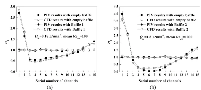
(a) (b)
Figure 7: Realization of uniform fluid flow distribution under different inlet flow-rate conditions: (a) Qin=0.18 L·min-1,
3
mean Rech=100; (b) Qin=1.8 L·min
-1
, mean Rech=1000.
4
Under low inlet flow-rate condition (Qin=0.18 L·min-1; mean Rech=100) with empty 5
baffle, the values of flow-rate are relatively high (σk>1.5) in channel 1 and 2 facing to the 6
inlet tube and then decrease rapidly to the lowest in channel 4, as shown in Fig. 7(a). After 7
that, a slow increase of flow-rate appears till the channel 15 which is the farthest channel 8
from the inlet tube. The flow distribution in the parallel channels is obviously non-uniform, 9
with the σk values ranging from 0.55 to 2.72 (PIV results). Meanwhile, CFD and PIV results 10
are in good agreement, implying that under low flow-rate condition, the laminar model is 11
capable of correctly simulating the fluid flow. With the insertion of the optimized baffle 1, the 12
fluid flow distribution among parallel channels is greatly homogenized and tends toward 13
uniform, indicated by a small variation of σk values (both CFD and PIV) around 1.0. The 14
maximum deviation θmaxamong 15 channels is lower than 5.0% and the corresponding MF
15
value is smaller than 0.02. 16
Figure 7(b) shows the CFD and PIV results on flow distribution under high inlet 17
flow-rate condition (Qin=1.8 L·min-1; mean Rech=1000). With the insertion of empty baffle, a 18
similar distribution curve may be observed compared to that under low-rate condition, the σk 19
values ranging from 0.04 to 4.00 (PIV results). CFD results are also in good agreement with 20
the PIV results for the general tendency, especially noticeable discrepancies for channels 5-9, 21
implying the potential difficulties in simulation caused by turbulence and vortex flows. Even 22
so, the insertion of the optimized baffle 2 serves as an optimized flow homogenizer to 23
improve the distribution uniformity, indicated by the decreased MF value from 1.100 to 0.041 24
(PIV results). For each channel, the maximum deviation θmaxalso decreases from 299.9% to
25
8.0% (PIV result). For the case of optimized baffle, CFD results show better agreement with 26
PIV results, indicated by almost flat distribution curves at σk=1.0. 27
12
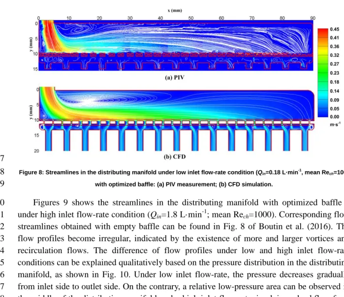
To better validate the CFD simulations by PIV measurement, an examination on the fluid 1
flow streamlines in the distributing manifold was carried out. Due to the limitation of view 2
field, the inlet distributing manifold was divided into seven independent parts which were 3
successively recorded by the CCD camera and then processed and connected so as to 4
reconstruct the fluid flow streamlines in the whole distributing manifold, except for a narrow 5
bar area which is not transparent due to the existence of the baffle. PIV and CFD results 6
under low inlet flow-rate conditions (Qin=0.18 L·min-1; mean Rech=100) with optimized 7
baffle 1 are presented in Fig. 8. Corresponding flow streamlines obtained with empty baffle 8
can be found in Fig. 7 of Boutin et al. (2016). 9
Under low inlet flow-rate condition, both the flow streamlines in the distributing 10
manifold obtained by PIV and CFD methods seem smooth and regular. A vortex next to the 11
inlet tube may be easily observed both on PIV and CFD images, with similar location and 12
size. This also explains the good agreement between PIV and CFD results on flow-rate 13
distribution among parallel channels. Due to the optimized dimensions of orifices on the 14
baffle, the fluid flow downstream the baffle is changed significantly so that a relatively 15
uniform fluid flow distribution is achieved. 16
17
Figure 8: Streamlines in the distributing manifold under low inlet flow-rate condition (Qin=0.18 L·min
-1
, mean Rech=100)
18
with optimized baffle: (a) PIV measurement; (b) CFD simulation. 19
Figures 9 shows the streamlines in the distributing manifold with optimized baffle 2 20
under high inlet flow-rate condition (Qin=1.8 L·min-1; mean Rech=1000). Corresponding flow 21
streamlines obtained with empty baffle can be found in Fig. 8 of Boutin et al. (2016). The 22
flow profiles become irregular, indicated by the existence of more and larger vortices and 23
recirculation flows. The difference of flow profiles under low and high inlet flow-rate 24
conditions can be explained qualitatively based on the pressure distribution in the distributing 25
manifold, as shown in Fig. 10. Under low inlet flow-rate, the pressure decreases gradually 26
from inlet side to outlet side. On the contrary, a relative low-pressure area can be observed in 27
the middle of the distributing manifold under high inlet flow-rate, implying a backflow from 28
outlet side to inlet side which that generates obvious vortices. The inserted perforated baffle 29
13
mainly influences the downstream pressure distribution to regulate the fluid flow-rates in 1
parallel channels. 2
With the optimized baffle 2, the sizes of the vortices in y direction are relatively smaller 3
because of the reduced available space in the distributing manifold upstream the baffle. 4
Similar to the cases for low inlet flow-rate condition, the locations of the vortices upstream 5
the baffle are not significantly changed with or without the insertion of baffle 2. Nevertheless, 6
because of optimized sizes of orifices, the fluid flow downstream the baffle is also controlled 7
to achieve uniform flow distribution, illustrating and confirming the effectiveness of the 8
geometrically optimized baffle insertion method. 9
10
Figure 9: Streamlines in the distributing manifold under high inlet flow-rate condition (Qin=1.8 L·min
-1
, mean Rech=1000)
11
with optimized baffle: (a) PIV measurement; (b) CFD simulation. 12
13
Figure 10: Pressure distributions in the distributing manifold. 14
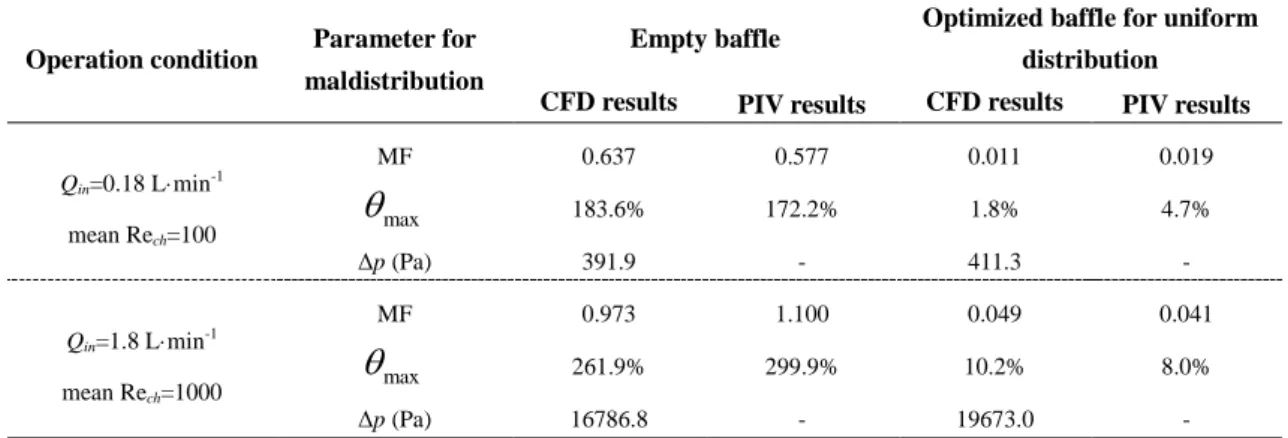
The values of MF and the maximum deviation for empty baffle 6 and for optimized 15
baffles 1 and 2 under different inlet flow-rate conditions are summarized in Table 2. It can be 16
observed that the flow distribution finally achieved is relatively more uniform under low 17
flow-rate condition than under high flow-rate condition. The precise control of fluid flow 18
14
becomes much more difficult due to the turbulent flow and the existence of various vortices, 1
leading to higher uncertainties in CFD simulations, in evolutionary algorithm and in PIV 2
measurement. Nevertheless, satisfactory results can still be obtained (MF<0.05, θmax about
3
10%) under high flow-rate condition and we are pretty sure that more satisfying results may 4
be achieved by employing advanced computational facilities and precise fabrication 5
techniques. Meanwhile, the total pressure drops of the fluidic network increase respectively 6
by 4.95% from 391.9 Pa (empty baffle) to 411.3 Pa (optimized baffle) under low inlet 7
flow-rate, and by 17.2% from 16786.8 Pa (empty baffle) to 19673.0 Pa (optimized baffle) 8
under high inlet flow-rate. Extra energy consumption is inevitable to change the initial fluid 9
flow distribution toward the target curve. 10
Table 2: Maldistribution factor (MF), maximum deviation (θmax) and total pressure drop of the fluidic network (Δp) for
11
empty baffle 6 and for optimized baffles 1 and 2 under different inlet flow-rate conditions 12
Operation condition Parameter for maldistribution
Empty baffle Optimized baffle for uniform distribution CFD results PIV results CFD results PIV results
Qin=0.18 L·min-1 mean Rech=100 MF 0.637 0.577 0.011 0.019 max 183.6% 172.2% 1.8% 4.7% Δp (Pa) 391.9 - 411.3 - Qin=1.8 L·min-1 mean Rech=1000 MF 0.973 1.100 0.049 0.041 max 261.9% 299.9% 10.2% 8.0% Δp (Pa) 16786.8 - 19673.0 -
4.2 Effective range of optimized baffle - a robustness study
13
In the above sub-section, it has been demonstrated that under the design flow-rate 14
conditions, the optimized baffles are really effective on the improvement of flow distribution 15
uniformity. Generally, it is recommended that the optimized baffle should work under its 16
design working condition and should be replaced by a new one when the operation condition 17
changes. In real-world engineering however, the workload (inlet flow-rate) may be fluctuant 18
so that the frequent replacement of baffle would become laborious, sometimes not 19
cost-effective. Actually small deviations from target flow distribution may be acceptable 20
when the tolerance on the distribution quality is relatively high. Therefore, it will be 21
interesting and of practical significance to test the robustness of the optimized baffle when 22
the inlet flow-rate deviates from its design value. 23
In this study, the optimized baffle 2 designed for uniform distribution (Qin=1.8 L·min-1; 24
mean Rech=1000) was tested both numerically and experimentally under other two inlet 25
flow-rate conditions, i.e. a lower flow-rate of 0.18 L∙min-1 (mean Rech=100) and a higher 26
flow-rate of 3.6 L∙min-1 (mean Rech=2000). Note that for this higher flow-rate, a gear pump 27
(MICROPUMP, O/CGC-M35.PVSF) with a measurement range of 1-5 L·min-1 and a flange 28
flowmeter (KOBOLD, DPL-1P15GL443) are used. PIV and CFD results on the flow 29
distribution among parallel channels obtained under different inlet flow-rate conditions are 30
shown in Fig. 11. It can be obviously observed that the flow distribution becomes less 31
15
uniform when the inlet flow-rate deviates from the design value. More precisely, when the 1
inlet flow-rate is reduced by a factor of 10 with respect to its design value (Qin=0.18 L·min-1 2
instead of 1.8 L·min-1; mean Rech=100 instead of 1000), the flow distribution curve appears 3
to be a parabolic shape, with the maximum in the middle channels (channels 6-7) and the 4
minimum on both sides (channels 1 and 15). Contrarily when the inlet flow-rate is doubled 5
(Qin=3.6 L·min-1 instead of 1.8 L·min-1; mean Rech=2000 instead of 1000), the actual 6
distribution curve appears to be a multi-segment line fluctuating around σk=1.0. 7
(a) (b)
Figure 11: Effective range tests for optimized baffle (design flow-rate of 1.8 L·min-1, mean Re
ch=1000): (a) lower flow-rate
8
(Qin=0.18 L·min
-1
, mean Rech=100); (b) higher flow-rate (Qin=3.6 L·min
-1
, mean Rech=2000).
9
The MF and θmax values for the optimized baffle 2 under different inlet flow-rate
10
conditions are listed in Table 3. It may be observed that the optimized baffle works less 11
effectively when the working condition deviates from its design value, indicated by larger 12
values of MF and θmax. When the inlet flow-rate is reduced by a factor of 10 (Qin=0.18
13
L·min-1), the MF value is smaller than 0.095 while the θmax value is lower than 15%. When
14
the inlet flow-rate is doubled (Qin=3.6 L·min-1), the MF value is smaller than 0.085 while the 15
θmax value is lower than 20%. Within a large variation range of inlet flow-rate (a factor of
16
0.1-2.0 with respect to the design value), the maximum deviation will rise to ±20%, which is 17
the double of that under design value (<±10%). However, compared to the empty baffle case 18
(with θmax higher than 170% at least), the distribution non-uniformity is still limited at a
19
relatively low level under our tested conditions by the insertion of a sub-optimal baffle.
20
Table 3: Maldistribution factor (MF) and maximum deviation (θmax) values for the same optimized perforated baffle under
21
different flow-rate conditions 22
Parameter for maldistribution
Baffle 2 (Rech=1000) Baffle 2 (Rech=100) Baffle 2 (Rech=2000)
CFD results PIV results CFD results PIV results CFD results PIV results
MF 0.049 0.041 0.093 0.090 0.085 0.065
max
10.2% 8.0% 14.1% 14.8% 19.6% 13.5%
23 24
16
Results shown in Fig. 11 also confirm the reliability of CFD simulations by PIV 1
measurement. Generally speaking, the results obtained by PIV and CFD are in good 2
agreement with each other, forming similar curves under the tested working conditions. Due 3
to the potential simulation errors, or the uncertainty in PIV measurement, the flow-rates in 4
some individual channels may be slightly different (e.g., channel 14 in Fig. 11(a), and 5
channel 3 in Fig. 11(b)). 6
4.3 Realization of non-uniform target flow distribution
7
In our previous work (Wei et al., 2015b), we have numerically demonstrated the 8
realization of non-uniform target flow distribution by the insertion of an optimized perforated 9
baffle, which has never been achieved by other conventional methods to the best of our 10
knowledge. In this sub-section, we try to validate this distinguished feature of our method by 11
testing two representative non-uniform target curves, i.e. a linear ascending and a linear 12
descending curve. These target curves are mathematically described in Table 1 and indicated 13
by hollow triangular symbols (∆) in the following figures. Corresponding perforated baffles 3 14
and 4 were optimized and fabricated, as shown in Table 1 and Fig. 4. These baffles were then 15
installed in the distributor section of the 15-channel fluidic network (Fig. 1) and PIV 16
measurements were performed under the inlet flow-rate Qin=0.18 L·min-1. The results of 17
empty baffle 6 under the same working condition were also used as the reference case for 18
comparison. 19
Figure 12 and Table 4 present the CFD and PIV results for realizing the ascending or 20
descending curve, using the optimized baffle 3 or 4, respectively. It can be seen that the CFD 21
results are in good agreement with the PIV measurements, approaching quite well the target 22
curves. Compared to the empty baffle 6 case, the MF value is reduced from about 0.7 to 23
smaller than 0.02 for the ascending target curve, and from about 0.6 to about 0.03 for the 24
descending target curve, by using the optimized baffles. The θmax value also decreases from
25
about 240% to lower than 4% for the ascending target curve, and from about 140% to lower 26
than 7% for the descending target curve. Moreover, the extra pressure drops caused by the 27
inserted perforated baffles are about 5% for both cases. Based on the results obtained above, 28
it is experimentally validated that the CFD-based evolutionary algorithm developed in Wei et 29
al. (2015b) is capable of realizing some non-uniform target flow distributions among parallel 30
channels. 31
It should be noted that these target curves proposed and tested here are just simple 32
examples. By a logical extension of this point, we are quite confident that other shapes of 33
target distribution curves can also be approached by the insertion of optimized perforated 34
baffles. For some extreme operation situations (e.g., step-like target curve) however, 35
complementary methods (e.g., partition walls, second baffle, etc.) may be necessary and this 36
issue will be further investigated in our future work. 37
17
(a) (b)
Figure 12: Realization of non-uniform target flow distribution using optimized perforated baffle (Qin=0.18 L·min-1, mean
1
Rech=100): (a) ascending target curve; (b) descending target curve.
2 3
Table 4: Maldistribution factor (MF), maximum deviation (θmax) and total pressure drop of the fluidic network (Δp) for
4
realizing non-uniform target flow distribution (Qin=0.18 L·min-1, mean Rech=100)
5
Parameter for maldistribution
Ascending target curve Descending target curve
Empty baffle 6 Optimized baffle 3 Empty baffle 6 Optimized baffle 4 CFD results PIV results CFD results PIV results CFD results PIV results CFD results PIV results MF 0.665 0.619 0.011 0.016 0.628 0.576 0.019 0.030 max 243.7% 201.4% 2.0% 3.5% 141.3% 111.6% 3.6% 6.5% Δp (Pa) 391.9 - 409.1 - 391.9 - 413.2 - 4.4 Discussions 6
A close investigation on the flow streamlines in the distributing manifold indicates that 7
the locations and sizes of vortices are influenced significantly by the total inlet flow-rate. The 8
discrepancies between CFD and PIV results under high flow-rate condition can be observed 9
due to the well-known difficulty of correctly modelling turbulent flow. Consequently, the 10
flow distribution optimization under high flow-rate conditions is relatively more difficult 11
because the evolutionary algorithm used to optimize the perforated baffles relies on CFD 12
simulation results. Therefore, high performance computational facilities are generally 13
required for more accurate simulation of fluid flow. Meanwhile, CFD results must be 14
validated by experimental measurements, especially under turbulent flow condition. 15
In our evolutionary algorithm, it is basically recommended that each optimized perforated 16
baffle works under its design flow-rate to reach the best performance on flow distribution. 17
However, a deviation of flow-rate with a factor of 0.1-2.0 from the design value will not 18
18
significantly influence the flow distribution uniformity under our tested conditions. Therefore, 1
the replacement of the perforated baffle can be performed according to the tolerance on flow 2
distribution quality and the costs. If the larger deviation from the target curve cannot be 3
accepted, a new perforated baffle has to be optimized and reinstalled. The proper design of 4
new perforated baffle calls for the running of whole optimization process which might be 5
time-consuming. Alternatively, some rapid designs may also be proposed following the 6
similar pattern or tendency of baffle configurations already obtained. 7
In actual applications, some practical issues must be carefully considered, such as the 8
orifice blocking or abrasion which may potentially modify the effective sizes of orifices on 9
the perforated baffles. These problems can be solved by adding a filter on the inlet tube or 10
using wear resistant materials for the fabrication of baffles. The flow distribution 11
optimization is a systematic task, not simply depends on local design or structural 12
optimization of the distributor. 13
5 Conclusion
14
In this paper, CFD simulations and experimental (PIV) measurements have been 15
performed in a 15-channel fluidic network to validate the realization of target flow 16
distribution by the method of geometrically optimized baffle insertion. CFD and PIV results 17
obtained indicate that various target flow distributions (uniform, ascending and descending 18
curves) can be approached under different inlet mass flow-rate conditions. Main conclusions 19
are summarized as follows: 20
Different CFD models used for simulations are validated by the PIV results. For 21
laminar flow, CFD simulation results (both flow distribution and streamlines) are in 22
excellent agreement with PIV measurements. For turbulent flow, CFD and PIV results 23
are also in good agreement with each other, but with a small deviation. 24
The realization of different target fluid flow distributions (uniform, ascending and 25
descending curves) by the insertion of geometrically optimized baffles is validated by 26
PIV measurement. The MF values can be reduced from more than 0.5 to less than 27
0.05 for all cases by using the optimized baffles. Likewise, the values of θmax are
28
reduced from more than 100% to less than 10%. 29
The robustness study implies that for uniform fluid flow distribution, the optimal 30
baffle can be used within a relative wide range of inlet flow-rate condition (by a factor 31
of 0.1 to 2.0 with respect to the design value), without affecting much the flow 32
distribution uniformity (MF<0.1). For non-uniform target distribution, the robustness 33
depends clearly on the shape of target curve so that the influences will be more 34
complex and should be tested case by case. 35
Note that the fluidic network used in this paper is just a model example without any 36
practical application background. The method of realizing target flow distribution by the 37
insertion of a geometrically optimized baffle, which has been proposed and developed in Wei 38
19
et al. (2015b) and validated experimentally in this study, can be applied in various 1
engineering fields dealing with fluid distribution problem. This will be the main direction of 2
our future work. 3
Acknowledgement
4
This work is financed by the BPI France and the Region Pays de la Loire, and monitored by 5
the SATT OUEST VALORISATION within the project OPTIFLUX (No. DV2054). One of 6
the authors M. Min WEI would also like to thank the French CNRS for its partial financial 7
support to his PhD study. The authors also thank Mr. Gwenaël BIOTTEAU and Mr. Nicolas 8
LEFEVRE for their great assistances during the device fabrication and the building of the 9
experimental set-up. 10
Notations
11
e depth of fluidic network m
m fluid mass flow-rate kg∙s-1
m target fluid mass flow-rate kg∙s-1
m average fluid mass flow-rate kg∙s-1
M total amount of parallel channels -
MF maldistribution factor -
Δp pressure drop Pa
Q volume flow-rate L∙min-1
Re Reynolds number -
12
Greek symbols 13
θmax maximum deviation -
σ flow-rate ratio - Subscripts ch channels in inlet k channel index
References
14Boerema, N., Morrison, G., Taylor, R., Rosengarten, G., 2013. High temperature solar thermal central-receiver
15
billboard design. Solar Energy, 97, 356-368.
16
Boutin, G., Wei, M., Fan, Y., Luo, L., 2016. Experimental measurement of flow distribution in a parallel
17
mini-channel fluidic network using PIV technique. Asia-Pacific Journal of Chemical Engineering, DOI:
18
10.1002/apj.2013
20 Carlomagno, G.M., Ianiro, A., 2014. Thermo-fluid-dynamics of submerged jets impinging at short
1
nozzle-to-plate distance: A review. Experimental Thermal and Fluid Science, 58, 15-35.
2
Fan, J., Furbo, S., 2008. Buoyancy effects on thermal behavior of a flat-plate solar collector. Journal Solar
3
Energy Engineering, 130, 021010–2.
4
Fan, Y., Boichot, R., Goldin, T., Luo, L., 2008. Flow distribution property of the constructal distributor and heat
5
transfer intensification in a mini heat exchanger. AIChE Journal, 54(11), 2796-2808.
6
Foucaut, J. M., Carlier, J., Stanislas, M., 2004. PIV optimization for the study of turbulent flow using spectral
7
analysis. Measurement Science and Technology, 8, 1427-1440.
8
Guo, X., Fan, Y., Luo, L., 2013. Mixing performance assessment of a multi-channel mini heat exchanger reactor
9
with arborescent distributor and collector. Chemical Engineering Journal, 227, 116-127.
10
Guo, X., Fan, Y., Luo, L., 2014. Multi-channel heat exchanger-reactor using arborescent distributors: A
11
characterization study of fluid distribution, heat exchange performance and exothermic reaction. Energy, 69,
12
728-741.
13
Kiger, K.T., Pan, C., 2000. PIV technique for the simultaneous measurement of dilute two-phase flows. Journal
14
of Fluids Engineering, 122(4), 811-818.
15
Lalot, S., Florent, P., Lang, S., Bergles, A., 1999. Flow maldistribution in heat exchangers. Applied Thermal
16
Engineering, 19(8), 847-863.
17
Lindken, R., Merzkirch, W., 2002. A novel PIV technique for measurements in multiphase flows and its
18
application to two-phase bubbly flows. Experiments in Fluids, 33(6), 814-825.
19
Luo, L., 2013. Heat and Mass Transfer Intensification and Shape Optimization: A Multi-scale Approach.
20
Springer, London.
21
Luo, L., Wei, M., Fan, Y., Flamant, G., 2015. Heuristic shape optimization of baffled fluid distributor for
22
uniform flow distribution. Chemical Engineering Science, 123, 542-556.
23
Meinhart, C.D., Wereley, S.T., Santiago, J.G., 1999. PIV measurements of a microchannel flow. Experiments in
24
Fluids, 27, 414-419.
25
Milman, O.O., Spalding, D.B., Fedorov, V.A., 2012. Steam condensation in parallel channels with nonuniform
26
heat removal in different zones of heat-exchange surface. International Journal of Heat and Mass Transfer, 55,
27
6054-6059.
28
Ong, B., Gupta, P., Youssef, A., Al-Dahhan, M., Dudukovic, M., 2009. Computed tomographic investigation of
29
the influence of gas sparger design on gas holdup distribution in a bubble column. Industrial & Engineering
30
Chemistry Research, 48(1), 58-68.
31
Ouyang, S., Li, X.G., Potter, O.E., 1995. Circulating fluidized bed as a catalytic reactor: experimental study.
32
AIChE Journal, 41(6), 1534-1542.
33
Rebrov, E.V., Schouten, J.C., De Croon, M.H.J.M., 2011. Single-phase fluid flow distribution and heat transfer
34
in microstructured reactors. Chemical Engineering Science, 66(7), 1374-1393.
21 Saber, M., Commenge, J.-M., Falk, L., 2010. Microreactor numbering-up in multi-scale networks for
1
industrial-scale applications: Impact of flow maldistribution on the reactor performance. Chemical Engineering
2
Science, 65(1), 372-379.
3
Salomé, A., Chhel, F., Flamant, G., Ferrière, A., Thiery, F., 2013. Control of the flux distribution on a solar tower
4
receiver using an optimized aiming point strategy: Application to THEMIS solar tower. Solar Energy, 94,
5
352-366.
6
Sehgal, S.S., Murugesan, K., Mohapatra, S.K., 2011. Experimental investigation of the effect of flow
7
arrangements on the performance of a micro-channel heat sink. Experimental Heat Transfer, 24, 215-233.
8
Sheng, J., Meng, H., Fox, R.O., 2000. A large eddy PIV method for turbulence dissipation rate estimation.
9
Chemical Engineering Science, 55(20), 4423-4434.
10
Siva, V.M., Pattamatta, A., Das, S.K., 2014. Effect of flow maldistribution on the thermal performance of
11
parallel microchannel cooling systems. International Journal of Heat and Mass Transfer, 73, 424-428.
12
Tarlet, D., Fan, Y., Roux, S., Luo, L., 2014. Entropy generation analysis of a mini heat exchanger for heat
13
transfer intensification. Experimental Thermal and Fluid Science, 53, 119-126.
14
Wei, M., Fan, Y., Luo, L., Flamant, G., 2015a. Fluid flow distribution optimization for minimizing the peak
15
temperature of a tubular solar receiver. Energy, 91, 663-677.
16
Wei, M., Fan, Y., Luo, L., Flamant, G., 2015b. CFD-based evolutionary algorithm for the realization of target
17
fluid flow distribution among parallel channels. Chemical Engineering Research and Design, 100, 341-352.
18
Wen, J., Li, Y., Zhou, A., Zhang, K., 2006. An experimental and numerical investigation of flow patterns in the
19
entrance of plate-fin heat exchanger. International Journal of Heat and Mass Transfer, 49, 1667-1678.
20
Westerweel, J., Elsinga, G.E., Adrian, R.J., 2013. Particle image velocimetry for complex and turbulent flows.
21
Annual Review of Fluid Mechanics, 45, 409-436.
22
List of figures
23
Figure 1: Geometry and dimensions of 15-channel fluidic network (unit: mm): (a) Parallelepiped A; (b)
24
Parallelepiped B; (c) Photo view after assembling; (d) Zoom on the inlet distributor and the location of the
25
perforated baffle. Adapted from Boutin et al. (2016).
26
Figure 2: Geometry and dimensions of the uniform baffle with identical width of orifices (unit: mm).
27
Figure 3: Width distribution of orifices on the baffles.
28
Figure 4: Photography of baffles used in this study.
29
Figure 5: Schematic diagram of the experimental setup built for this study.
30
Figure 6: Experimental workbench for subtle movements of the test-section.
31
Figure 7: Realization of uniform fluid flow distribution under different inlet flow-rate conditions: (a) Qin=0.18
32
L·min-1, mean Rech=100; (b) Qin=1.8 L·min-1, mean Rech=1000.
22 Figure 8: Streamlines in the distributing manifold under low inlet flow-rate condition (Qin=0.18 L·min-1, mean
1
Rech=100) with optimized baffle: (a) PIV measurement; (b) CFD simulation.
2
Figure 9: Streamlines in the distributing manifold under high inlet flow-rate condition (Qin=1.8 L·min-1, mean
3
Rech=1000) with optimized baffle: (a) PIV measurement; (b) CFD simulation.
4
Figure 10: Pressure distributions in the distributing manifold.
5
Figure 11: Effective range tests for optimized baffle (design flow-rate of 1.8 L·min-1, mean Rech=1000): (a)
6
lower flow-rate (Qin=0.18 L·min-1, mean Rech=100); (b) higher flow-rate (Qin=3.6 L·min-1, mean Rech=2000).
7
Figure 12: Realization of non-uniform target flow distribution using optimized perforated baffle (Qin=0.18
8
L·min-1, mean Rech=100): (a) ascending target curve; (b) descending target curve.
9
List of tables
10
Table 1: Target curves and design flow-rates for different perforated baffles
11
Table 2: Maldistribution factor (MF), maximum deviation (θmax) and total pressure drop of the fluidic network
12
(Δp) for empty baffle 6 and for optimized baffles 1 and 2 under different inlet flow-rate conditions
13
Table 3: Maldistribution factor (MF) and maximum deviation (θmax) values for the same optimized perforated
14
baffle under different flow-rate conditions
15
Table 4: Maldistribution factor (MF), maximum deviation (θmax) and total pressure drop of the fluidic network
16
(Δp) for realizing non-uniform target flow distribution (Qin=0.18 L·min-1, mean Rech=100)