Numerical simulation of air flow with different roof configuration

READ THESE TERMS AND CONDITIONS CAREFULLY BEFORE USING THIS WEBSITE.

https://nrc-publications.canada.ca/eng/copyright

Vous avez des questions? Nous pouvons vous aider. Pour communiquer directement avec un auteur, consultez la Questions? Contact the NRC Publications Archive team at

PublicationsArchive-ArchivesPublications@nrc-cnrc.gc.ca. If you wish to email the authors directly, please see the first page of the publication for their contact information.

NRC Publications Archive

Archives des publications du CNRC

This publication could be one of several versions: author’s original, accepted manuscript or the publisher’s version. / La version de cette publication peut être l’une des suivantes : la version prépublication de l’auteur, la version acceptée du manuscrit ou la version de l’éditeur.

Access and use of this website and the material on it are subject to the Terms and Conditions set forth at

Numerical simulation of air flow with different roof configuration

Kashef, A.; Baskaran, B. A.

https://publications-cnrc.canada.ca/fra/droits

L’accès à ce site Web et l’utilisation de son contenu sont assujettis aux conditions présentées dans le site LISEZ CES CONDITIONS ATTENTIVEMENT AVANT D’UTILISER CE SITE WEB.

NRC Publications Record / Notice d'Archives des publications de CNRC:

https://nrc-publications.canada.ca/eng/view/object/?id=7eeca88a-0b5a-46a3-8fba-db8146091b45 https://publications-cnrc.canada.ca/fra/voir/objet/?id=7eeca88a-0b5a-46a3-8fba-db8146091b45

91CWE. i'J95. Nc:....· Delhi. India

NUMERICAL SIMULATION OF AIR FLOW WITH

DIFFERENT ROOF CONFIGURATIONS FOR THE

PREDICTION OF SNOW ACCUMULATION

KASHEF, AHMED and BASKARAN. BAS A.

ｒｾｳｲｩＱｮ［ｨｵｳＮ ｉｉｉｓＬｩＯｗｉｾＯｯｲ Rtstan;hinCOIIS/ruc/ioll, NOlional Rtuo.rrh COlUlc:i1 Co.fIlJda. 0110.1\'0. On/ario. CtJIltJda. KIA OR6.

Abstract

Applying Computational Fluid Dynamics (CFD) technique, numerical investigations have been carried out to simulate wind flow conditions on various roof configurations. Using the computed mean wind flow field, the snow-drift distributions on these roof configurations are calculated. This study demonstrates that the CFD technique can be effectively applied in the earty stage of the design process as a predictive tool for forecasting snow accumulation

on various roof configurations. Efforts are also made to quantify the validity of model

predictions through comparisons with field observation and wind tunnel data.

1. INTRODUCTION

Wind and snow play an important role in many design aspects of the building envelope. Thorough understanding of mean wind flow behavior as well as the ability to quantitatively predict it, is indispensable for forecasting snow-drifting distribution. Snow accumulations on roofs are usually quantified by gathering field data which often involves a prohibitive high cost. The knowledge can be instead obtained through wind tunnel experiments on small·scale models. Recently, CFD technique vies for lead as a new method of analysis to understand and quantify wind flow conditions around buildings.

Studies applying the CFD technique for wind flow modeling were recently reviewed by

Baskaran and Stathopoulos (1994). The majority of the studies computed the wind flow

conditions for buildings with flat roofs. Stathopoulos and Zhou (1993) computed the mean

wind induced pressures on a step roof configuration. On the other hand, architectural

features such as parapets can significantly alter the local flow conditions over

a

roof

(Baskaran, 1986). Recent wind tunnel and full scale studies revealed that scale effect and pressure tap locations are critical in predicting these effects (Kind, 1988and Stathopoulos and Marathe, 1993). Numerical models are not restricted by the scale effect. Therefore, present study attempts to investigate the applicability of CFD to study the effect of roof architectural

features on the local mean wind flow conditions. The data acquired by the numerical

696 simulation is configurations. 2. TECHNICI 2.1 Air FlowI Compl uses the Can equations inti several thou transferred b well-known ｾ is used.- Th assumed prE" Besid PHOENICS prepared. It for building conditions, (

as

GROUNI selection 0 modificatior Performanc Council Ca hard diskSI 2.2 Snow

Snc

wind actiol place. SOl force has expressec (ground c dragged I layer abo compute environm determinl H; calculate U/U' = 2 where l acceler.:

2. TECHNIOUES AND TOOLS USED

simulation is further utilized to predict snow·drift distributions on various building toof configurations.

Where U is the wind velocity at any given height z above the snow surface and g is the acceleration due to gravity, 9.81 mls. Due to the implicit nature of Eq. 1, the determination of (1)

691 U/u°=2.5 In (2gzlU°2j

+

9.7

2.2 Snow accumulation calculations

Snow-drifting refers to the movement of loose snow lying on the ground surface by wind action. As a result of snow-drifting, significant re·distribution of the snow mass can take place. Snow particles are moved by the drag force associated with the moving air. The drag force has to overcome the inter-particle cohesive forces between snow particles, conveniently expressed by U*th, the threshold shear velocity. Snow is mainly transported by ·saltation"

(ground drift) (Kind, 1985). In this process, the heavy snow particles are bounced and

dragged near the ground surface. The movement of the particles which takes place in a thin

layer above the ground level is called the saltaUon layer. The general procedure used to

compute the snow accumulation involves the following steps: (1) simulation of the wind environmental conditions to obtain the friction velocity (U*) at each nodal point; (2) determination of snow transport rate; and (3) estimation of erosion or deposition rates.

Having determined the mean velocity field from CFD simulation, the friction velocity is calculated using the following equation produced by Owen (1964)

2.1 Air Flow modeling

Computations were made using the CFD solver PHOENICS (Spalding, 1981) which uses the Control Volume Method (CVM). The CVM converts the non-linear partial differential equati6ns into difference equations. The solution of the difference equations is obtained at several thousand control volume nodes such that the satisfaction of the momentum transferred between the control volumes is guaranteed. To fulfill the continuity of mass, the well-known Semi-Implicit Pressure Linked Equations (SIMPLE) algorithm of Patankar (1980) is used: These, in tum, enable one to correct the velocity field and improve the initially assumed pressure field.

Besides the customizing procedures, two major sutr-modules are needed to use PHOENICS for current wind flow modeling. First, the input module, known as the Q1 file, is prepared. It consists of computational domain sizes, details for grid arrangement, coordinates for building locations and 'other computational parameters such as values for initial !low conditions, convergence criteria and relaxation factors. Second, the boundary module, known as GROUND, is carefully formulated. It includes the specification of boundary conditions, the

selection of necessary numerical schemes and turbulence models. Details of these

modifications are reported in CHAM (1993). All computations were pertormed. at the Building Performance Laboratory of the Institute for Research in Construction· National Research Council Canada using a HP 735 (36 MFLOPS) computer system with 48 MB RAM and 2 GB hard disk storage.

q = C (pig) (IW,II U'lh) U'2 (U'lh • U') (2)

u

a _{involves an iterative process. The snowdrift transport rate q, due to the saltation}

phenomenon, is then calculated by the following equation, (Uematsu et ai, 1991)

where p is the air density ( 1.2 kgfm

3). C

is an empirical constant (1.0). and Wf is the snow particle tenninal velocity. Finally, the snowdrift rate s (mass of snow accumulating on unit horizontal area) is calculated as

Where h is the height of the saltation layer.

The snow depth, H. can be calculated by converting the snowdrift rate, s, using a proportionality parameter a (H= a s), where a equals (HO/sO); HO is the obselVed snow depth at an open area free of obstacles and SO is the calculated snowdrift rate at the same point as

w.

performed se tunnel with 1;: heights; 6 ani that in suburl with speeds

c

A30r flow fields ha' terminal velo( the experimf turbulence in level and Wf roof for both (3)

• = •

(qIW,II U h)

3. RESULTS AND DISCUSSION

3.1 Efforts to quantify the model validity

The main object of the present study is to identify the effect of roof architectural features on snow accumulation. As was discussed in the section 2.2. to be able to calculate the snow-drift one should first determine the local mean wind speed. In the present study, this has been successfully accomplished through the use of the CFD solver PHOENICS. It should be recognized that PHOENICS uses the k-E turbulence model along with first principle momentum and mass equations to simulate the wind flow conditions around buildings. Murakami (1992) compared the relative performance of k-E turbulence model with the algebraic second-moment closure (ASM) and large eddy simulation (LES) in predicting turbulent flow fields around a bluff body. The mean wind flow fields produced by the three

models are compared with the wind tunnel results. Murakami concluded that the three

turbulence models produced a fairly good agreement with the wind tunnel testing with respect

to the mean velocity vector field. Therefore. it has been decided to use PHOENICS as a

solver in the present study. Moreover, Baskaran and Said (1993) investigated the application of PHOENICS for modeling air flow conditions through building envelope. Simulated results produced by a 3D time-dependent model was compared with experimental data collected through controlled laboratory conditions. Comparisons reflected a good agreement between the experimental data and numerical modeling results.

Efforts have been made to quantify the validation of the present snow accumulation predictions. Experimental snow studies at the NaJional Research Council Canada between

1974.and 1982 accumulated data on snow load on roofs (Taylor. 1985). They prOVide

extensive field data for codification purposes. However, an extensive literature review by the present study revealed the lack of complete information sets (wind velocity and turbulence intensity profiles, bUildings geometry, snow type, snow particles characteristics and etc.) that can be specified as inlet and outlet boundary conditions for the model simulations.

. Some results from wind tunnel model tests carried out by Morrison et al (1981) were used In an effort to quantify the validity of the model predictions. Morrison et al (1981)

Figure'

The numbl the numer similar tot

7JJrnji

•

\'

, ,

,

,

I

ｾｾ

I

""

...

),,:\

5.6m/.

Comparison of snow accumulation between numerical simulation and \'.ind tunnel experiments

Figure 1

performed several model tests using sand-water analogue of snow-drifting in a water flume tunnel with 1:200 scale. A square building with dimensions of 25 m by 25 m with two different heights; 6 and 30 m was used for the tests. Approaching wind profile was representative of that in suburban areas and was expressed as a power law with an exponent equal to 0.25 with speeds of 5.6 m1s and 7.0 mls at roof levels of 6 and 30 m respectively.

A 3D numerical model was developed to calculate the snow-drift distributions from wind flow fields having a similar configuration to the wind tunnel tests. Turbulence intensity profile, terminal velocity of snow particle

CWf}

and height of saltation layer (h) were not available from

the' experimental study. Therefore, they were assumed in the numerical simulation:

turbulence intensity varies from 22% to 5% over a height 20 m to 200 m above the ground level and Wf as 0.5 m1s and h as 1.0 m. Computed contour plots for snow accumulation on roof for both investigated buildings are presented in Figure 1 together wah wind-tunnel data.

•

The num.bers on the figure represent snow depths in units of 0.1 meters. For both heights. the numerical model found to be capable of predicting the trend of snow-drift distribution similar to the measurements. For building with height 30 m, computed trends compare better with the corresponding wind tunnel data than in the case of building with height 6 m. This

FE:

observation ratifies the fact that the scale effect on the wind tunnel study might be stronger on lower heights results than at 30 m height. The discrepancy between wind tunnel and model results can beattributed to the assumptions made in the model dUB to non availability of the comprehensive experimental data.

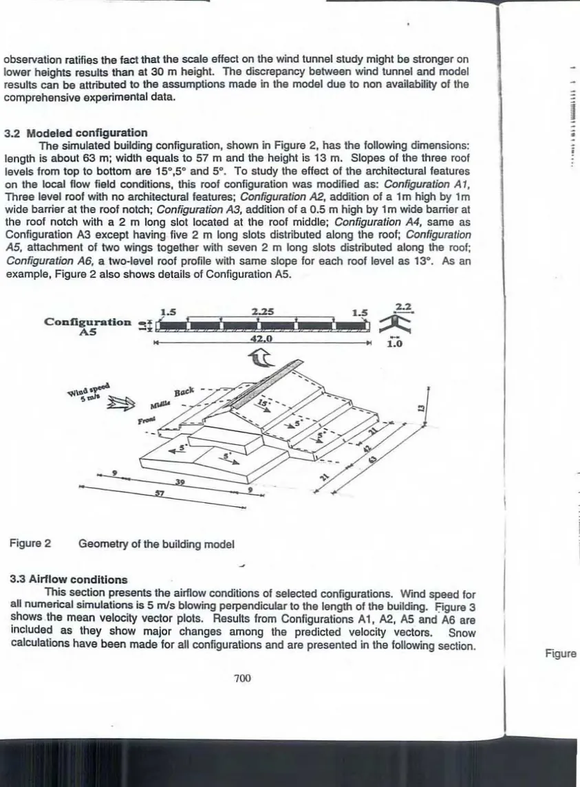
3.2 Modeled configuration

The simulated building configuration, shown in Figure 2, has the following dimensions: length is about 63 m; width equals to 57 m and the height is 13 m. Slopes of the three roof levels from top to bottom are 15°,5° and 5°. To study the effect of the architectural features on the local flow field conditions, this roof configuration was modified as: Configuration A 1, Three level root with no architectural features; Configuration A2, addition of a 1m high by 1m wide barrier at the roof notch; Configuration A3, addition of a 0.5 m high by 1m wide barrier at

the roof notch with a 2 m long slot located at the roof middle; Configuration A4. same as

Configuration A3 except having five 2 m long slots distributed along the roof; Configuration

AS, attachment of two wings together with seven 2 m long slots distributed along the roof;

Configuration A6, a two-level roof profile with same slope for each roof level as 130

• As an

example, Figure 2 also shows details of Configuration A5.

1.5 2.2. _1.' 2.2 Configuration

ｾｩｦ［

₁

•

•

•

1

I

ｾ

A5 II 42,0 .1 _1.0

4

-I

.

i

-,

-;

.

Figure 2 Geometry of the building model

3.3 Airflow conditions

This section presents the airflow conditions of selected configurations. Wind speed for all numerical simulations is 5 mls blowing perpendicular to the length of the building. Figure 3 ｾｨｯｷｳ the mean velocity vector plots. Results from Configurations Al, A2, AS and"A6 are

Included as they show major changes among the predicted velocity vectors. Snow

calculations have been made for all configurations and are presented in the following section.

---,

,

_•

; ;

,

,

i

co ft all AI: ""-,:,, ,;j;;,;,ii

n gur

on

ｾ ＺＧｾ［Ｚ［ｊＯＨ［Ｚ［ＭＧＺﾷｩｲＮＺＮﾷＯ

, ;

i

:,;;:.:;,ii;,;;;n;,;;;,iJiffflflii!f!t(J.;ffflffi/';;H;i'iUi:_{... ,,,,,,It_,,!!.. ,,,,,·,,,·,,}

_{.,'tI.',,,,,,,}

_,,,,,ti,,,,,

COnftguratlon

1.2

- -

-

---_

..

_---Velocity vector plots at middle sections for Configurations A1, A2, AS and A6

- -

_--

-

-;;;

;;; ;;;

-"

"

; ｾ

•

-ｾ

;;

; _. .

,

refrence veloctty 20

mIl

>

IUUUU

---iiii ..

iii;ii";;o;;;:--

,

ｾＬＮＺ［ＮＮ

...

""

,

［ｩｬｩｩｩｩｬｬＬｾｾｾｩｊｊｬｬｬｬｬｩ

;; §

ｾ ｾ ｾ

f ;:

.,=

ｾＮＺＬＺ Ｏ［ＨＮｾｾＮｩＮｩＮｩﾷﾷｾﾷＺﾷＺａＺﾷ［ﾷＺＺｾｾｾｾｾｾｾｾｲＺｾｾｾＺｾＮｾＥ＿［［Ｎ

.:-

ｾＬＮｾ

;; ;; .. ; ;

!

ｾ

ii ;;: -

',.

-I. I :

Contlgwatlon At

ｾＧＺ ＮＺ［ｾＮＬＯＭＺＮＺＭＢＢＬＧＮｾＮＺＮ

=

i. ,:,1:' .iUt " .... ".,./"""" •• , J • . .,':"!!' . :"',:_.' ..'.'.': , ' . ".".:':.:j!.';;!:i.:

J.'.','.'.'!

f••.:'ｾ:".'.",'.'

'.'.!!.',', '.',',','',':".',','',"

'-t': tｪＯＯｩｾｾ ｾ［Ｌ ｾＬ .ih,I:i"l,It ..",."Ii:" "Ilei. . ::,": n",,,ItitT::

'It"," "' .""''''

tI,.,j" "",,1,1/,,,'I, II

All vector plots are shown by taking a vertical plane passing through the middle of the building (Figure 2) with a reference velocity of 20 mls. Only those vectors in the building proximity are displayed to get a better insight of the flow conditions in the vicinity of the building. In Figure 3, longer vectors indicate higher wind speed. Flow separation points from the windward flow, changes in wind directions along the three slopes of the roof and wake regions behind the building, are clearly predicted by the model and are shown in the figure.

In Configuration A:2, presence of the solid barrier at rool notch, significantly reduce the velocity values on leeward side. An area of recirculation has been created immediately after the barrier and extends up to the roof lowest level. The velocity vectors for AS show that the size of the recirculation zone is smaller than A:2. As shown in Figure 2, Configuration AS, has two wings and a slope along the barrier. Wind coming from left passes through the slots and obstructed by the wing on the right hand side. This creates the so-called 'jet effect' at the roof

top as shown by the vector plots. By changing the roof profile to a two-level roof, as in

Configuration AG, the airflow field is significantly modified as compared to Configurations which are three-level roof (A 1, A:2, and AS). In this case the locations of separation and recirculations are adjusted to the new roof profile. Recirculation zones smaller in size are only observed at the vertical junction between the two roof levels. It is evident from the figure that for AG, wind speeds are higher and, in general, separation of flow is more distinct and extends to a longer distance in the leeward side in comparison to A 1, A2 and AS.

3.4 Snow accumulation for different configurations

Using the above computed mean wind flow field, snowdrift distributions on the roofs of all investigated configurations are calculated and presented in this section.

Figures 4. 5 and G summarize the results of snowdrift distribution for Configurations A1 and A2, A3 and A4, and AS and AG respectively. Each figure displays the distributions at the front, middle and back sections of the building model (ref. Rgure 2). Only snow accumulation at the building leeward side roof is presented acknowledging that the effect of air1low on snow, mainly, occurs on that side. The x-axis represents a cross section through the building in a distorted scale. Snow accumulations are drawn to scale in the vertical axis. These curves are not connected at junctions of the roofs because there is no snow accumulation calculated at vertical places connecting roof levels.

Figures 4 through Greveals that:

• An average of 100, 90 and 10 em of snow accumulation is predicted on first, second and

third level respectively for A 1 (Rgure 4). The lower the roof the larger the accumulation. These results confinn with the field observations which indicated an average snow accumulation 100 em on the lower roof level (Roger, 1994).

• A significant increase in the depth of accumulated snow on the top roof level is observed for A2 (Figure 4). Asimplied by the results of airflow analysis, this is due to reduction in

the local velocity field and developed recirculation regions. An average accumulation

depth of 100 em is forecasted to all the three"'roof levels.

• Snow·drift distributions for A3 and A4 (Figure 5) are similar at the middle section. Major changes of snow·drift distribution are observed only on the top roof level.

• For Configuration AG, the overall distribution of snow accumulation on the top roof level is lower than the rest of the configurations. This is because of the high wind flow field on bUilding roof level produced in this case. On the other hand, distribution of snow on the lower roof level is quite similar to those for other modifications.

J

1.0

ｏｾｾｦＬｬＺ

1.0

09<'"L-.0 0 '",-,:, 1.0

ｏｾＧｴ

'" 0

ＧＧＧＺｾｾ

0 0 .

o

L-. 0

<p...

0

ＢＢＧｏＮｾ

ｾ

tJ1a4:'"

0

or.

0 0 Y'.·

b

0

］

ｾｃｬｴｬ］ｾｏｕＢＧﾷＧ

0

ｏｵＮｾ

0 =O.u . <Q 0 0

l14b·o

" 0 0 0,.0 0.0 112 0 0

"

n n

u. 1.0 ConfigurationA2 Solid Barrier ".0 06:'1> ' 0 1.0 ＼ｬＺｾＧ 0 _

o

0 0

I""'.

CIl4;J' 0 -""6 0

o

0 V " O ' I i , O " . O O L... (\ (f"' 0

_o.u

·<QOO " 0 Con!igumlionAl 1.0 0.8 1.0 0.6

ｾ

1.0

ｾ ｾｾ

•

Ｌ｢ｴｾ

I'\,.

0:'

11,£,J;oii:ll.

ｊＮＮＮＮＮＮＱＧ［ＺｪＡＢｩｏｏｾ

I

ｾ

0

ｾ

P:

ｾ

u.u n

oil::

ｾ ｏｾ

U.IT

=

ｉｲｆＭｲｯＭＭＭＧｮＭｴＭｳＭ･｣ＮｌｴｩＭﾷＭｯｮＧｾ

1.0

0.'

0.'

ｾ

0.'

[ 0.0.2 "

I:h"

o. .

Figure 4

I

Middle Sectio.;J

,

ConfigurationA3

Solid BamerwithOne slot _{Solid Bamer}Configuration A4_{withS Slots}

1.0 M

...

...

_0.2

='=0»

1.0 M ...

...

ｾＮ

I

ｾ

ｾＮ

ｾｾｾ

.

ｾｾｾｉｉＺＲ［ＬｩＺＺｪｮｴ［

_...

ｾ 1.0 Figure 5

I

Middle Section

I

1.0 M

0.'

ｾ 0t 1.0

ｾ

ＰｾＱｾｾ

ｾｾｬｬｾｾＺ

ｏｾＺ

... c!'!

ｏｾｬ

ＰｾｾＰＱ

u.u ｯｾ 0 =1,..

ConfigurationAS _{ConfigmatiooA6}

Two Wmgs with Seven Slots _{Two-level Roof Profile}

ｬｾ _1.0

.

...

0.8 1.0 0.• _'.0 0.6

O.

ｉｾ 0.'

_Oo&W

OA

10

0

•

0

•

0.6 0.8

"

ｯｾＦ

_0.2

ｲＱａＱｾ

D••

1='=

° °

ﾰｯｾＮｴ

Jo • °

:bOv 0.0

Jo°OOO

ｉＢｾ

n

,..f:4I

_°

_｡ｾ

ｾ

n

_{° 0}

v.v [.Ill! u.

n

_°

-

: b ==

I

Front Section

I

1.0 1.0 0.8 0.8 0.' 1.0

If:c,

0.• -.1.0

1°

0 [ .

[):

IE

0

ｾ

0.'

-"',:.

:aPo

o

ｏｾｬ

ｾ

_{o a}.}

_{° 08.1\}

l d

,

00

ｾ

I

Ｎｾ

ｯＺｾ

°

0.0 .... n 0

6

==0.

'. '0

0:'

°

Ｎｾ

°0

ｾ

I

&2

°

00.

01

_°

'4,

• n

ｯｾ 0

_°

₀ v, 0

°

.

•

•

• ==

==

IMiddle S=tionl

ｉｾ 1.0

...

0.8 U 0.• _1.0 0.6

ｾ

0°0 ,n 0.'

ｾ

0°

0.'

ｾ

,.,,02

oOe

-

0.2

_o

_.6 ｜ｬＩｾ

_°

00

-:bOo _ｾ

o

0 0.0 _00. ｜ｬｬｾ _",0f!.

_{ｾＢＧｳＴ}

_°

ﾰｮ｡ｾ

_ﾰｮｾ

•

0 V.V

c<U

₀ 0.0

•

n

='=

.

==

I

Back: S=tion

I

Figure 6

To identify the best configuration with regard to minimum snow accumulation, one should examine both air flow conditions and snow calculations. For A6. the air flow analysis (Figure 3) implies that the reattachment of flow occurs well before the lower roof edge. Thus the major portion of accumulated snow on lower roof will be driven to the ground by the

gravity and high roof profile slope (15°). The snow removal process is augmented, in this

case, by wind driving forces. The gravity effect is not considered in the numerical modeling and thus it is not reflected in snow predictions. Whereas for the other configurations, the major part of the lower roof level (with slope of 5°) is subjected to negative flow. These recirculations, by acting against the gravity effect, may keep the snow on the roof. Thus one

can select A6 as the optimum design for minimum snow accumulation. For owners and

developers such optimum design can be obtained by having detennined the dominant wind directions and the wind profile for a given location. Investigation of this nature demonstrates the benefit of applying CFD technique at the early design stage.

4. CONCLUDING REMARKS

Numerical tests carried out in the presented study clearly demonstrated the suitability of applying the CFD techniques, as useful tool, for the investigation of wind flow conditions on building roofs with various architectural features. CFD can also be used as a predictive tool to

forecast snow accumulation. Conclusions fonnulated based on the numerical study are

presented below:

• Application of CFD techniques for predicting wind flow field provides various modification opportunities for the owners and developers during the early design stage of the building roof configuration.

• Sophisticated CFD solvers such as PHOENICS requires qualified personnel to specify the

appropriate boundary and inlet conditions as well to interpret the simulation results.

• A calculation procedure for snow-drift distribution is under development. At present, it can forecast snow accumulation trends over various roof configurations. The predicted trends are in agreement with field data. Further, quantification of the predictions can only be made if data collected from identical experimental setup is available. It is worthy to initiate a systematic experimental program to generate such controlled data.

5. REFERENCES

Baskaran, A. and Said, M. N. A. (1993), ·Application of CFD to Investigate Buildings Airflow·,

Proceedings of Conference of the CFD, Society of Canada, Montreal, June 14-15, pp.

207-219.

Baskaran, A. and Stathopoulos, T. (1994), ·Prediction of Wind Effects on BUildings Using Computational Methods - State of The Art Review·, Canadian Journal of Civil Engineering, to be published in the October issue.

Baskaran, A. (1986), ·Wind Loads On Flat Roofs With Parapets·, M. Eng. (Building) Thesis, Concordia University, Montreal, Canada.

CHAM I H Kind, R F

1

Kind, R

,

Morriso J I Murak. Owen, Patanl Roger Spaid Stath Stath Taylc Uem ACI

The

fan Natf

ACKNOWLEDGMENT

The authors acknowledge Public Works and Government Services Canada (Mr. F. Pelletier), for whom the present study was carried out. The authors thank Mr. P. Roger, Department of National Defense, for providing snow accumulation field data.

CHAM Development Team (1993), rrhe PHOENICS - 2.0 User Guide-, CHAM, Bakery

House, 40 High Street, Wimbledon, London SW19 5AU, UK.

Kind, R. J. (1985),·Snow-Drifting: A Review of the Process and Modeling Methods·, Snow Property Measurements Workshop, Lake Louise, Alberta, Technical Memorandum

140,1-3 April.

Kind, R. J. (1988), ·Worst Suctions Near Edges Of Flat Rooftops With Parapets·, J. Wind Eng. and Ind. Aerodynamics, Vol. 31, pp 251-264.

Morrison, Hershfield, Theakston and Rowan, Limited (1981), ·Prevention of Excess Snow Accumulation due to Roof Mounted Solar Collectors·, A Housing Energy Management Program Report prepared for the Ministry of Municipal Affairs and Housing, ISBN

0-n43-706B-B.

Murakami, S. (1992). ·Comparison of Various Turbulence Models Applied to a Bluff Body", First International Symposium on Computational Wind Engineering, Tokyo, CWE 92, pp

164-179.

Owen, P. R. (1964), ·Saltation of Uniform Grains in Ai"", Journal of Fluid Mechanics. Vol. 20,

pt. 2, pp 225-242.

Patankar. S.V. (1980), ·Numerical Heat Transfer and Fluid Flow" Hemisphere Publishing Corporation, McGraw-Hili Book Company.

Roger, P. (1994), Private Communications, Department of National Defense, Ottawa, Ontario, Canada.

Spalding, D. B. (1981), ·A General Purpose Computer Program for Multi-Dimensional One and Two·Phase Flow·, Math. and Camp. Simulation, Vol. XXIII, pp 267-276.

Stathopoulos, T. and Marathe, R. (1993),· Field Measurements of Wind Induced Pressures on Roofs Of Low Buildings·, ASCE Structures Congress, Irvine, CA, April, PP 18-21. Stathopoulos, T. and Zhou, Y. (1993), ·Computation of Wind Pressures on L - Shaped

Buildings·, Journal of Engineering Mechanics, ASCE, Vol. 119, No.8, pp 1526-1641. Taylor, D. A. (1985), -Snow Loads on Slopping Roofs: Two Pilot Studies in the Ottawa Area·,

Canadian Journal of Civil Engineering, Vol. 12, pp 334·343.

Uematsu, T., Nakata, T., Takeuchi,

K.,

Arisawa, Y.and Kaneda, Y. (1991), ·Three·dimensional Numerical Simulation of SnowdriW, Cold Regions Science and Technology, Vol. 20, pp