HAL Id: cea-02339617
https://hal-cea.archives-ouvertes.fr/cea-02339617
Submitted on 4 Nov 2019
HAL is a multi-disciplinary open access
archive for the deposit and dissemination of sci-entific research documents, whether they are pub-lished or not. The documents may come from teaching and research institutions in France or abroad, or from public or private research centers.
L’archive ouverte pluridisciplinaire HAL, est destinée au dépôt et à la diffusion de documents scientifiques de niveau recherche, publiés ou non, émanant des établissements d’enseignement et de recherche français ou étrangers, des laboratoires publics ou privés.
Verification of iterative matrix solutions for multipoint
kinetics equations
J. Tommasi, G. Palmiotti
To cite this version:
J. Tommasi, G. Palmiotti. Verification of iterative matrix solutions for multipoint kinetics equations. Annals of Nuclear Energy, Elsevier Masson, 2018, 124, pp.357-371. �cea-02339617�
Page 1 sur 31
Verification of iterative matrix solutions for multipoint kinetics equations
Jean Tommasi
CEA, DEN, DER, SPRC, Cadarache, F-13108 Saint Paul lez Durance, France Giuseppe Palmiotti
Idaho National Laboratory, 2525 Fremont Ave. P.O. Box 1625, Idaho Falls, ID 83415-3860 (USA)
Abstract
Multipoint kinetic equation systems have been solved numerically using matrix algebra
software and 1st to 4th order implicit schemes based on single-step matrix propagators.
These matrix schemes have been validated successfully on demanding point kinetics benchmarks with various prescribed reactivity insertions. Verification tests have also been performed on a simple 3-region fast reactor core model with asymmetric step or ramp reactivity insertions and cross-checked with the multipoint kinetics SACRE code developed at INL and based on existing and validated stiff ODE solver packages. Accurate results can be obtained at a limited time expense. The reason for intriguing results obtained in some transients has been elucidated and linked to the multipoint matrix coefficient interpolation method during the transient.
Keywords: multipoint kinetics equations, implicit matrix methods 1. Introduction
Multipoint kinetics (MPK) is a description tool for the change in time of the neutron field in a nuclear reactor, intermediate between the point kinetics (PK) description that neglects any change in the spatial distribution of the flux and a full space (3D) + time kinetic description of the reactor. The system is divided in several fissile regions, each considered as a separate point reactor and connected to others by coupling coefficients and neutron generation times. Prompt and delayed neutrons are accounted for. It is believed that, provided the number and extension of the regions have been chosen with physical insight in connection to the response sought for, MPK can capture many features of real kinetic transients.
The first multipoint model was derived by Avery (Avery, 1958) in view of application to the design of a coupled fast-thermal reactor. Spatial integrations on regions, to obtain the multipoint variables and coefficients, are performed after multiplication by weight functions with physical meaning. Avery used weight functions connected to the classical adjoint flux (neutron importance). An alternate form was derived by Kobayashi (Kobayashi, 1991), using Green functions related to the production of next generation neutrons. Avery’s and Kobayashi’s models are multipoint in space only, but models multipoint in space and in energy have been proposed also (Bosio et al., 2001; Ravetto et al, 2004). Avery and Kobayashi provided a technique to compute the coupling coefficients between zones using deterministic codes, but another possibility is to use pragmatic definitions for the coupling coefficients, based on probabilities, opening the way to their computation by Monte-Carlo estimators (Aufiero et al. 2016; Laureau et al. 2017a&b).
Page 2 sur 31
We will restrict here to space multipoint models. The goal of the present study was to build a simple and quick, but nevertheless accurate, tool to compute prescribed transients on multipoint core models, with possible further extensions to transients with feedback. Such a tool could be used to gain insight on the quantitative time behaviour of spatially decoupled cores (zero power experimental reactors with very different and coupled regions, large industrial cores). Using matrix algebra software, this tool will be tagged as MATMPK in the following for quick reference. Another incentive to develop MATMPK was to provide comparison terms with the existing MPK code, named SACRE, developed independently at INL (Palmiotti et al., 2018) and help in understanding puzzling results obtained by the latter (Palmiotti et al., 2018, and see below).
The kinetic equations describing the evolution of the neutron flux Ψ(𝑟⃗, 𝐸, Ω⃗⃗⃗, 𝑡) and the
concentrations of the 𝐷 ≥ 1 families of delayed neutron precursors 𝐶(𝑖)(𝑟⃗, 𝑡) may be
written as the following system of (1 + 𝐷) equations:
{ 1 𝑣 𝜕Ψ 𝜕𝑡 = (𝐅𝑝− 𝐀)Ψ + ∑ 𝜒𝑑(𝑖)𝜆(𝑖)𝐶(𝑖) 𝐷 𝑖=1 𝑑𝐶(𝑖) 𝑑𝑡 = ∫ 𝜈𝑑(𝑖)Σ𝑓Ψ 𝑑𝐸𝑑2Ω − 𝜆(𝑖)𝐶(𝑖) (1)
F is the operator governing the neutron production by fission, i.e. the sum of 𝐅𝑝 (prompt
fission production operator) and 𝐅𝑑 (delayed fission production operator). A is the
operator grouping the scattering, streaming and collision terms:
𝐅𝑝Ψ = 𝜒𝑝(𝐸, Ω⃗⃗⃗) ∫ 𝑑𝐸′ 𝑑2 Ω′ 𝜈𝑝(𝑟⃗, 𝐸′, 𝑡) Σ𝑓(𝑟⃗, 𝐸′, 𝑡)Ψ(𝑟⃗, 𝐸′, Ω⃗⃗⃗′, 𝑡) (2) 𝐅𝑑Ψ = ∑ 𝜒𝑑(𝑖)(𝐸, Ω⃗⃗⃗) ∫ 𝑑𝐸′ 𝑑2 Ω′𝜈 𝑑(𝑖)(𝑟⃗, 𝐸′, 𝑡) Σ𝑓(𝑟⃗, 𝐸′, 𝑡)Ψ(𝑟⃗, 𝐸′, Ω⃗⃗⃗′, 𝑡) 𝐷 𝑖=1 (3) 𝐀Ψ = Ω⃗⃗⃗ ∙ ∇⃗⃗⃗Ψ + Σ𝑡Ψ − ∫ 𝑑𝐸′𝑑2Ω′ Σ 𝑠(𝑟⃗, 𝐸′ → 𝐸, Ω⃗⃗⃗′→ Ω⃗⃗⃗)Ψ(𝑟⃗, 𝐸′, Ω⃗⃗⃗′) (4)
Fission spectrum normalization is: ∫ 𝑑𝐸𝑑2Ω 𝜒(𝐸, Ω⃗⃗⃗) = 1 (5)
Eq.(1) is a system of coupled equations for the neutron flux and the precursor concentrations. But hereafter, for quick reference, any equation containing the time derivative of the flux will be called a flux equation, and any equation containing the time derivative of a precursor concentration will be called a precursor equation. In equation systems such as Eq.(1), only one line for the flux equations and one line for the precursor equations will be written; indices will avoid confusion (e.g. the second line in Eq.(1) being indexed by (𝑖), represents 𝐷 precursor equations)
The classical derivation of PK equations, dating back to (Henry, 1958) is reminded in Appendix. The multipoint equations are derived in Section 2 for Avery’s and Kobayashi’s models, together with the definition of all the coupling coefficients and the way these coefficients can be approximated for their calculation in deterministic codes.
Page 3 sur 31
Assuming the coupling coefficients, produced by any suitable method, are available, the PK and MPK variables obey systems of linear ordinary differential equations: (1 + 𝐷) equations for PK and, if 𝑁 is the number of fissile regions 𝑁(1 + 𝐷) equations for Kobayashi’s MPK formulation and 𝑁(𝑁 + 𝐷) equations for Avery’s MPK formulation. These linear systems can be cast in a vector-matrix format, and Section 3 presents the derivation of approximate single-step matrix propagators over a time interval ∆𝑡: those yielding the well-known first (implicit Euler) and second (Crank-Nicolson) order methods, and two more complex ones, based on Newton-Cotes quadrature formulas, resulting in third and fourth order methods. In this same section, a short reminder of the structure and capabilities of the SACRE code developed at INL is provided.
The free and open source software Scilab (Scilab Enterprises, 2012) has been used to code these matrix propagators in order to test and validate them. Scilab is used as a toolbox for fast (compiled) and accurate solvers for matrix algebra operations, here mainly matrix product, inversion and exponentiation. Its interpreted user’s language has been used to write scripts performing all ancillary tasks (fill in the matrices, organize the loops and tests, call the built-in pre-compiled functions, print the results). Section 4 presents the verification of MATMPK on demanding PK benchmarks (Ganapol, 2013), with benchmark 10-digit objective values for three kinds of prescribed reactivity injection (step, ramp, sinusoidal). Attention is given on accuracy vs. time step size, and
to CPU times. In Section 5 a simple 3-region fast reactor model with 2/3 rotation
symmetry in its reference configuration is defined; the kinetic transients are based on extraction of a single control rod, breaking the symmetry of the core. The coupling coefficients necessary to MATMPK are computed using the ERANOS code system (Ruggieri et al., 2006), and two simple verification tests are performed: a step insertion (the control rod is extracted instantaneously) and a ramp insertion (progressive extraction of the control rod). The step insertion can be validated against an analytical solution obtained by matrix exponentiation; for the ramp insertion, a qualitative match with physical insight is sought for. With respect to the previous PK benchmarks, additional attention is given to shape variations, i.e. the progressive change in the balance of fission rates in the three fissile regions of the core. Finally, Section 6 is devoted to the comparison of results provided by MATMPK and SACRE on a same 3-region problem. In addition, the reason for intriguing results previously obtained by SACRE when modelling the same transient by various methods (PK, MPK with various subdivisions of the reactor into regions) has been elucidated and linked to the multipoint matrix coefficient interpolation method used during the transient.
2. Derivation of the multipoint equations
The usual technique (Henry, 1958; Avery, 1958; Komata, 1969; Kobayashi, 1992) is to multiply the kinetics equations Eq.(1) by one or several weight functions and to integrate over space, energy and angle. We shall use the following notation for the functional scalar product so defined:
Page 4 sur 31
The usual derivation of PK equations (Henry, 1958) is recalled in Appendix. The weight function used in this case is a critical adjoint flux, and the lumped parameter obtained from the neutron flux is called the neutron population or amplitude. In the MPK models of Kobayashi and Avery, the lumped parameters obtained from the neutron flux are more directly related to region-wise fission source rates.
2.1. Kobayashi’s MPK equations
The system is partitioned into 𝑁 distinct fissile regions. 𝛿𝑛 is the function equal to 1 in
region 𝑛, 0 elsewhere. The precursor concentrations, divided into 𝐷 time families, are split into:
𝐶(𝑖) = ∑ 𝐶
𝑛(𝑖) 𝑁
𝑛=1 with 𝐶𝑛(𝑖) = 𝛿𝑛𝐶(𝑖) (𝑖 = 1, ⋯ , 𝐷) (7)
Each of the 𝐷 precursor equations is split into 𝑁 equations (by multiplication by the 𝛿𝑛),
so that Eq.(1) can be written as the following system of 1 flux equation and 𝑁𝐷 precursor equations : { 1 𝑣 𝜕Ψ 𝜕𝑡 = 𝐅𝑝Ψ − 𝑨Ψ + ∑ 𝜆(𝑖)𝜒𝑑(𝑖)∑ 𝐶𝑛(𝑖) 𝑁 𝑛=1 𝐷 𝑖=1 𝑑𝐶𝑛(𝑖) 𝑑𝑡 = ∫ 𝜈𝑑(𝑖)Σ𝑓𝑛Ψ 𝑑𝐸𝑑2Ω − 𝜆(𝑖)𝐶𝑛(𝑖) (8)
where Σ𝑓𝑛 = 𝛿𝑛Σ𝑓 is the restriction of the fission cross-section to region 𝑛. For the flux
equations a weight function 𝑊𝑚 is defined for each region and we obtain the following
set of 𝑁(1 + 𝐷) equations (𝑁 flux equations and 𝑁𝐷 precursor equations):
{ < 𝑊𝑚, 1 𝑣 𝜕Ψ 𝜕𝑡 > = < 𝑊𝑚, 𝐅𝑝Ψ > − < 𝑊𝑚, 𝑨Ψ > + ∑ 𝜆(𝑖)∑ < 𝑊𝑚, 𝜒𝑑(𝑖)𝐶𝑛(𝑖) > 𝑁 𝑛=1 𝐷 𝑖=1 <𝑑𝐶𝑛 (𝑖) 𝑑𝑡 > = < 𝜈𝑑(𝑖)Σ𝑓𝑛Ψ > − 𝜆(𝑖) < 𝐶𝑛(𝑖) > (9)
(for 𝐶𝑛(𝑖) integration is on space only). The weight function 𝑊𝑚 chosen by Kobayashi is
the function 𝐺𝑚+ obeying the source equation:
𝐀+𝐺
𝑚+ = 𝜈Σ𝑓𝑚 (10)
This choice is meant to make the term < 𝑊𝑚, 𝑨Ψ > in Eq.(9) equal to the fission source
in region 𝑚, 𝑆𝑚 = < 𝐅𝑚Ψ > (𝐅𝑚 = 𝛿𝑚𝐅 is the restriction of the production operator to
region 𝑚), which will be one of the unknowns of the final MPK set of equations:
< 𝐺𝑚+, 𝐀Ψ > = < 𝐀+𝐺𝑚+, Ψ > = < 𝜈Σ𝑓𝑚Ψ > = < 𝐅𝑚Ψ > = 𝑆𝑚 (11)
By its definition in Eq.(10), 𝐺𝑚+(𝑟⃗, 𝐸, Ω⃗⃗⃗), defined over the whole system, represents the
expected value for the number of neutrons produced at next generation in region 𝑚 for
1 current generation neutron placed at (𝑟⃗, 𝐸, Ω⃗⃗⃗).
The other terms in Eq.(9) can be worked out as follows (definitions for the integral kinetics parameters are given directly in the equations) :
Page 5 sur 31 < 𝐺𝑚+, 𝐅 𝑝Ψ > = ∑ < 𝐺𝑚+, (𝐅 𝑛− 𝐅𝑑𝑛)Ψ > < 𝐺𝑚+, 𝐅 𝑛Ψ > ∙ < 𝐺𝑚+, 𝐅 𝑛Ψ > < 𝐅𝑛Ψ > ∙< 𝐅𝑛Ψ > 𝑁 𝑛=1 ≝ ∑(1 − 𝛽𝑚𝑛)𝑘𝑚𝑛𝑆𝑛 𝑁 𝑛=1 (12)
𝑘𝑚𝑛 is the expected number of neutrons produced at next generation in region 𝑚 for 1
neutron produced at current generation in region 𝑛 and is called a coupling coefficient;
the matrix K such as 𝐾𝑚𝑛 = 𝑘𝑚𝑛 being called the coupling matrix. 𝛽𝑚𝑛 is the fraction of
delayed neutrons produced at next generation in region 𝑚 by neutrons produced at current generation in region 𝑛 due to delayed neutrons produced at current generation in region 𝑛. < 𝐺𝑚+, 1 𝑣 𝜕Ψ 𝜕𝑡 > = < 𝐺𝑚+,1 𝑣𝜕Ψ𝜕𝑡 > < 𝜕(𝐅𝑚Ψ) 𝜕𝑡 > < 𝜕(𝐅𝑚Ψ) 𝜕𝑡 > ≝ ℓ𝑚 𝑑𝑆𝑚 𝑑𝑡 (13)
ℓ𝑚 has the dimensionality of time. It is the ratio of the number of neutrons produced at
next generation in region 𝑚 by excess neutrons originating from the whole system to the increase of production rate in region 𝑚, and may be considered an average time needed by prompt neutrons to reach region 𝑚 and generate next generation neutrons.
∑ 𝜆(𝑖)∑ < 𝐺 𝑚+, 𝜒𝑑(𝑖)𝐶𝑛(𝑖) > 𝑁 𝑛=1 𝐷 𝑖=1 = ∑ 𝜆(𝑖)∑< 𝐺𝑚+, 𝜒𝑑(𝑖)𝐶𝑛(𝑖)> < 𝐶𝑛(𝑖) > < 𝐶𝑛 (𝑖)> 𝑁 𝑛=1 𝐷 𝑖=1 ≝ ∑ 𝜆(𝑖)∑ 𝑘 𝑚𝑛(𝑖) < 𝐶𝑛(𝑖) > 𝑁 𝑛=1 𝐷 𝑖=1 (14)
𝑘𝑚𝑛(𝑖)is the expected number of neutrons produced at next generation in region 𝑚 for 1
delayed neutron of family 𝑖 produced at current generation in region 𝑛; we can also
group them into matrices 𝐊(𝑖) called delayed coupling matrices.
< 𝜈𝑑(𝑖)Σ𝑓𝑚Ψ > = < 𝜈𝑑
(𝑖)Σ
𝑓𝑚Ψ >
< 𝐅𝑚Ψ > ∙< 𝐅𝑚Ψ > ≝ 𝛽𝑚(𝑖)𝑆𝑚 (15)
𝛽𝑚(𝑖) is the raw delayed neutron fraction for family 𝑖 in region 𝑚. The 𝑁(1 + 𝐷)
Kobayashi multipoint equations are then, keeping the notation 𝐶𝑚(𝑖) for < 𝐶𝑚(𝑖)>:
{ ℓ𝑚𝑑𝑆𝑚 𝑑𝑡 = (1 − 𝛽𝑚) ∑ 𝑘𝑚𝑛𝑆𝑛 𝑁 𝑛=1 − 𝑆𝑚+ ∑ 𝜆(𝑖)∑ 𝑘 𝑚𝑛(𝑖)𝐶𝑛(𝑖) 𝑁 𝑛=1 𝐷 𝑖=1 𝑑𝐶𝑚(𝑖) 𝑑𝑡 = 𝛽𝑚 (𝑖)𝑆 𝑚− 𝜆(𝑖)𝐶𝑚(𝑖) (16)
So far, all the involved coefficients are written using the unknown dynamic flux Ψ(𝑡),
but they can be approximated by using instead of the static flux of the associated
critical problem, solution of
(𝐅
Page 6 sur 31
the operators being taken at current time. For the generation times, we assume an asymptotic exponential regime where the derivatives of funtions are proportional to the functions themselves, with identification of the time eigenfunction with the multiplication factor eigenfunction of Eq.(17). This way we obtain the following set of approximate point kinetic parameters for the Kobayashi equations:
𝑘𝑚𝑛 ≈<𝐺𝑚+,𝐅𝑛Φ> <𝐅𝑛Φ> 𝑘𝑚𝑛 (𝑖) ≈<𝐺𝑚+,𝐅𝑑𝑛(𝑖)Φ> <𝐅𝑑𝑛(𝑖)Φ> 𝛽𝑚𝑛 ≈ <𝐺𝑚 +,𝐅 𝑑𝑛Φ> <𝐺𝑚+,𝐅𝑛Φ> 𝛽𝑚 (𝑖) ≈<𝜈𝑑(𝑖)Σ𝑓𝑚Φ> <𝐅𝑚Φ> ℓ𝑚≈ <𝐺𝑚+,1𝑣Φ> <𝐅𝑚Φ> (18) 2.2. Avery’s MPK equations
With respect to the Kobayashi approach, the neutron flux is also split into a sum of
partial fluxes:
Ψ = ∑ Ψ𝑛
𝑁
𝑛=1
(19)
Here Ψ𝑛 is defined as the partial flux due to only the neutrons (prompt and delayed)
produced in region 𝑛. Hence, the kinetic equations, Eq.(1), become the following system of 𝑁(1 + 𝐷) equations (𝑁 flux equations + 𝑁𝐷 precursor equations):
{ 1 𝑣 𝜕Ψ𝑛 𝜕𝑡 = 𝐅𝑝𝑛Ψ − 𝑨Ψ𝑛+ ∑ 𝜒𝑑(𝑖)𝜆(𝑖)𝐶𝑛(𝑖) 𝐷 𝑖=1 𝑑𝐶𝑛(𝑖) 𝑑𝑡 = ∫ 𝜈𝑑(𝑖)Σ𝑓𝑛Ψ 𝑑𝐸𝑑2Ω − 𝜆(𝑖)𝐶𝑛(𝑖) (20)
In the flux equations, the prompt and delayed fission neutron sources are strictly
localized to region 𝑛, but as operator A includes spatial derivatives, the Ψ𝑛 are non-zero
over the whole system (although they may decrease sharply outside region 𝑛). When
starting from an initial static critical configuration Ψ0 = Φ0, the initial values of the
partial fluxes, Ψ𝑛0, are solution of the 𝑛 sub-critical source problems
(𝐀0− 𝐅𝑝𝑛0)Ψ𝑛0= ∑ 𝜒𝑑(𝑖)𝜆(𝑖)𝐶 𝑛0(𝑖) 𝐷 𝑖=1 with 𝐶𝑛0(𝑖) = 𝜈𝑑(𝑖)Σ𝑓𝑛0Φ0 𝜆(𝑖) (21)
Here again, we associate to each region 𝑚 = 1, ⋯ , 𝑁 a weight function 𝑊𝑚 defined over
the whole system and we integrate to obtain the following system of 𝑁(𝑁 + 𝐷)
equations (𝑁2 flux equations + 𝑁𝐷 precursor equations:
{ < 𝑊𝑚,1 𝑣 𝜕Ψ𝑛 𝜕𝑡 > = < 𝑊𝑚, 𝐅𝑝𝑛Ψ > − < 𝑊𝑚, 𝑨Ψ𝑛 > + ∑ 𝜆(𝑖) < 𝑊𝑚, 𝜒𝑑(𝑖)𝐶𝑛(𝑖) > 𝐷 𝑖=1 < 𝑑𝐶𝑚 (𝑖) 𝑑𝑡 > = < 𝜈𝑑(𝑖)Σ𝑓𝑚Ψ > −𝜆(𝑖) < 𝐶𝑚(𝑖) > (22)
Page 7 sur 31
We could use also here the weight functions defined by Kobayashi in Eq.(10), but Avery
followed another path. His choice for the weight function 𝑊𝑚 is a multiple of the “partial
static adjoint flux” Φ𝑚+ solution of the source equation
𝐀+Φ 𝑚 + =𝛿𝑚 𝑘𝑐 𝐅+Φ+ = 1 𝑘𝑐𝐅𝑚+Φ+ (23)
Where Φ+ is a fundamental solution of the associated adjoint critical problem:
(𝐅
+
𝑘𝑐 − 𝐀
+) Φ+ = 0 (24)
(this is the equation adjoint to Eq.(17)). By construction, we have:
∑ Φ𝑚+
𝑁
𝑚=1
= Φ+ (25)
Then, through simple algebraic manipulations:
< Φ𝑚+, 𝐀Ψ 𝑛 > = < 𝐀+Φ𝑚+, Ψ𝑛 > = 1 𝑘𝑐 < 𝐅𝑚 +Φ+, Ψ 𝑛 > = 1 𝑘𝑐 < Φ +, 𝐅 𝑚Ψ𝑛 > (26)
The multiplicative coefficient 𝛼𝑚 in 𝑊𝑚= 𝛼𝑚Φ𝑚+ is chosen to ensure a summation to
the fission source of region 𝑚 as follows:
𝛼𝑚 𝑘𝑐 ∑ < Φ+, 𝐅𝑚Ψ𝑛 > 𝑁 𝑛=1 =𝛼𝑚 𝑘𝑐 < Φ+, 𝐅𝑚Ψ > = < 𝐅𝑚Ψ > ⇒ 𝛼𝑚 = 𝑘𝑐 < 𝐅𝑚Ψ > < Φ+, 𝐅 𝑚Ψ > (27)
Then we can define the partial fission sources, which will be part of the unknowns in the final MPK equations, as:
𝑆𝑚𝑛 = < 𝐅𝑚Ψ >∙< Φ+, 𝐅 𝑚Ψ𝑛 > < Φ+, 𝐅 𝑚Ψ > 𝑆𝑚 = ∑ 𝑆𝑚𝑛 𝑁 𝑛=1 = < 𝐅𝑚Ψ > (28)
𝑆𝑚𝑛 can be interpreted as the part of the fission rate 𝑆𝑚 due to only the neutrons
originated by neutrons produced in region 𝑛. The first term in the right hand side of the flux equations in Eq.(22) can be developed as:
𝑘𝑐 < Φ𝑚+, 𝐅 𝑝𝑛Ψ > < 𝐅𝑚Ψ > < Φ+, 𝐅 𝑚Ψ > =< Φ𝑚 +, 𝐅 𝑛Ψ > − < Φ𝑚+, 𝐅𝑑𝑛Ψ > < Φ𝑚+, 𝐅𝑛Ψ > ∙ 𝑘𝑐 < 𝐅𝑚Ψ >∙< Φ𝑚+, 𝐅 𝑛Ψ > < 𝐅𝑛Ψ >∙< Φ+, 𝐅𝑚Ψ >∙ < 𝐅𝑛Ψ > ≝ (1 − 𝛽𝑚𝑛)𝑘𝑚𝑛𝑆𝑛 (29)
Page 8 sur 31 𝑘 < Φ𝑚+,1 𝑣 𝜕Ψ𝑛 𝜕𝑡 > < 𝐅𝑚Ψ > < Φ+, 𝐅 𝑚Ψ >= 𝑘 < Φ𝑚+,1𝑣𝜕Ψ𝜕𝑡 >𝑛 𝑑𝑆𝑚𝑛 𝑑𝑡 < 𝐅𝑚Ψ > < Φ+, 𝐅 𝑚Ψ >∙ 𝑑𝑆𝑚𝑛 𝑑𝑡 ≝ ℓ𝑚𝑛𝑑𝑆𝑚𝑛 𝑑𝑡 (30)
ℓ𝑚𝑛 has the dimensionality of time and may be considered an average time needed by
neutrons born in region 𝑛 to reach region 𝑚 and generate next generation neutrons. The coupled flux-precursor term is developed as:
𝑘 < Φ𝑚+, 𝜒𝑑(𝑖)𝐶𝑛(𝑖)> < 𝐅𝑚Ψ > < Φ+, 𝐅 𝑚Ψ >= 𝑘 < Φ𝑚+, 𝜒 𝑑 (𝑖)𝐶 𝑛(𝑖)> < 𝐶𝑛(𝑖)> < 𝐅𝑚Ψ > < Φ+, 𝐅 𝑚Ψ >∙< 𝐶𝑛 (𝑖) > (31)
and written, with notation abuse (𝐶𝑛(𝑖) for < 𝐶𝑛(𝑖) >):
< Φ𝑚+, 𝜒 𝑑 (𝑖)𝐶 𝑛(𝑖) > < 𝐅𝑚Ψ > < Φ+, 𝐅 𝑚Ψ >≝ 𝑘𝑚𝑛 (𝑖)𝐶 𝑛(𝑖) (32)
In the precursor equations we define also: < 𝜈𝑑(𝑖)Σ𝑓𝑚Ψ > =< 𝜈𝑑
(𝑖)Σ
𝑓𝑚Ψ >
< 𝜈Σ𝑓𝑚Ψ > ∙< 𝜈Σ𝑓𝑚Ψ > ≝ 𝛽𝑚(𝑖)𝑆𝑚 (33)
Finally, the 𝑁(𝑁 + 𝐷) Avery MPK equations are:
{ ℓ𝑚𝑛𝑑𝑆𝑚𝑛 𝑑𝑡 = (1 − 𝛽𝑚𝑛)𝑘𝑚𝑛𝑆𝑛− 𝑆𝑚𝑛+ ∑ 𝜆(𝑖)𝑘𝑚𝑛(𝑖)𝐶𝑛(𝑖) 𝐷 𝑖=1 𝑑𝐶𝑚(𝑖) 𝑑𝑡 = 𝛽𝑚(𝑖)𝑆𝑚− 𝜆(𝑖)𝐶𝑚(𝑖) (34)
The formal manipulations leading to the sources and coefficients defined in Eq.(28, 29,
30, 32, 33) involve the unknown kinetic flux . These coefficients are approached using
the static flux of the associated critical problem, Eq.(17), and its partial fluxes:
𝐀Φ𝑚 = 1 𝑘𝑐𝐅𝑚Φ (35) We have then: 𝑆𝑚𝑛 ≈<𝐅𝑚Φ>∙<Φ+,𝐅𝑚Φ𝑛> <Φ+,𝐅 𝑚Φ> 𝑘𝑚𝑛 ≈ 𝑘𝑐 <𝐅𝑚Φ>∙<Φ𝑚+,𝐅𝑛Φ> <𝐅𝑛Φ>∙<Φ+,𝐅𝑚Φ> 𝛽𝑚𝑛 ≈ <Φ𝑚+,𝐅𝑑𝑛Φ> <Φ𝑚+,𝐅𝑛Φ> 𝛽𝑚 (𝑖) ≈<𝜈𝑑(𝑖)Σ𝑓𝑚Φ> <𝐅𝑚Φ> (36)
For the 𝑘𝑚𝑛 coefficients, through the definition of partial fluxes Eq.(23, 35):
< Φ𝑚+, 𝐅
𝑛Φ > = 𝑘𝑐 < Φ𝑚+, 𝐀Φ𝑛 > = 𝑘𝑐 < 𝐀+Φ𝑚+, Φ𝑛 >
= < 𝐅𝑚+Φ+, Φ𝑛 > = < Φ+, 𝐅𝑚Φ𝑛 > (37)
This relation allows falling back on Avery’s definition for the 𝑘𝑚𝑛 (Avery, 1958):
𝑘𝑚𝑛 ≝ 𝑘𝑐 < 𝐅𝑚Φ >∙< Φ+, 𝐅 𝑚Φ𝑛 > < 𝐅𝑛Φ >∙< Φ+, 𝐅𝑚Φ > = 𝑘𝑐 𝑆𝑚𝑛 𝑆𝑛 (38)
Page 9 sur 31
For the generation times, an asymptotic exponential regime is assumed, where the derivatives are proportional to the functions, and the time eigenfunction is identified with the multiplication factor eigenfunction:
ℓ𝑚𝑛 ≈ 𝑘 < Φ𝑚+,1 𝑣 Φ𝑛 > 𝑆𝑚𝑛 < 𝐅𝑚Φ > < Φ+, 𝐅 𝑚Φ >= 𝑘 < Φ𝑚+,1 𝑣 Φ𝑛 > < Φ+, 𝐅 𝑚Φ𝑛 > (39) And finally, the precursor distribution is assumed proportional to the neutron production distribution of the associated critical problem:
𝑘𝑚𝑛(𝑖) ≈ 𝑘𝑐< 𝐅𝑚Φ >∙< Φ𝑚+, 𝐅𝑑𝑛
(𝑖)Φ >
< 𝐅𝑑𝑛(𝑖)Φ >∙< Φ+, 𝐅
𝑚Φ >
(40)
2.3. Formal comparisons of the MPK models
2.3.1. Basic features
Table 1 recapitulates the number of equations, weight functions and approximate formulations for kinetic coefficients based on the calculation of static fluxes.
Table 1 – Multipoint model comparison
Kobayashi Avery 𝑁(1 + 𝐷) equations 𝑁(𝑁 + 𝐷) equations Weights: 𝐺𝑚+ 𝐀+𝐺 𝑚+ = 𝜈Σ𝑓𝑚 Weights: Φ𝑚+ 𝐀+Φ 𝑚+ = 1 𝑘𝐅𝑚+Φ+ ℓ𝑚 ≈ < 𝐺𝑚+,1 𝑣 Φ > < 𝐅𝑚Φ > ℓ𝑚𝑛 ≈ 𝑘 < Φ𝑚+,1 𝑣 Φ𝑛 > < Φ+, 𝐅 𝑚Φ𝑛 > 𝛽𝑚𝑛 ≈< 𝐺𝑚+, 𝐅𝑑𝑛Φ > < 𝐺𝑚+, 𝐅 𝑛Φ > 𝛽𝑚𝑛 ≈ < Φ𝑚+, 𝐅𝑑Φ𝑛 > < Φ𝑚+, 𝐅Φ 𝑛 > 𝑘𝑚𝑛 ≈ < 𝐺𝑚+, 𝑭𝑛Φ > < 𝐅𝑛Φ > 𝑘𝑚𝑛 ≈ 𝑘 < 𝐅𝑚Φ >∙< Φ+, 𝐅 𝑚Φ𝑛 > < 𝐅𝑛Φ >∙< Φ+, 𝐅 𝑚Φ > 𝑘𝑚𝑛(𝑖) ≈< 𝐺𝑚 +, 𝐅 𝑑𝑛 (𝑖)Φ > < 𝐅𝑑𝑛(𝑖)Φ > 𝑘𝑚𝑛 (𝑖) ≈ 𝑘< 𝐅𝑚Φ >∙< Φ𝑚+, 𝐅𝑑𝑛 (𝑖)Φ > < 𝐅𝑑𝑛(𝑖)Φ >∙< Φ+, 𝐅 𝑚Φ > 𝛽𝑚(𝑖) ≈< 𝜈𝑑 (𝑖)Σ 𝑓𝑚Φ > < 𝐅𝑚Φ > 𝛽𝑚(𝑖) ≈ < 𝜈𝑑(𝑖)Σ𝑓𝑚Φ > < 𝐅𝑚Φ >
2.3.2. Reduction of Avery’s model to Kobayashi’s model Summing the 𝑛 Avery flux equations having 𝑚 as first index yields:
Page 10 sur 31 ∑ ℓ𝑚𝑛𝑑𝑆𝑚𝑛 𝑑𝑡 𝑁 𝑛=1 = ∑(1 − 𝛽𝑚𝑛)𝑘𝑚𝑛𝑆𝑛 𝑁 𝑛=1 − 𝑆𝑚+ ∑ 𝜆(𝑖)∑ 𝑘 𝑚𝑛(𝑖)𝐶𝑛(𝑖) 𝑁 𝑛=1 𝐷 𝑖=1 (41) This means that we can have a formal identification to Kobayashi’s model (at a given moment) if: ℓ𝑚 ≡ ∑ ℓ𝑚𝑛𝑑𝑆𝑚𝑛 𝑑𝑡 𝑁 𝑛=1 ∑ 𝑑𝑆𝑚𝑛 𝑑𝑡 𝑁 𝑛=1 (42)
This agrees with the interpretations of ℓ𝑚𝑛 as the average time needed for neutrons
born in region 𝑛 to reach region 𝑚 and produce next generation neutrons, and ℓ𝑚 as the
average time for neutrons born in the whole system to reach region 𝑚 and produce next generation neutrons.
2.3.3. Reduction of multipoint to point model
For a single region (𝑁 = 1), both Kobayashi and Avery sets of equations reduce to:
{ ℓ 𝑑𝑆𝑑𝑡 = [(1 − 𝛽)𝑘 − 1]𝑆 + ∑ 𝜆(𝑖)𝑘(𝑖)𝐶(𝑖) 𝐷 𝑖=1 𝑑𝐶(𝑖) 𝑑𝑡 = 𝛽(𝑖)𝑆 − 𝜆(𝑖)𝐶(𝑖) (43)
If we divide the first equation by 𝑘ℓ and multiply the precursor equations by 𝑘𝑘ℓ(𝑖) we get:
{ 𝑑𝑆 𝑑𝑡 = 𝜌 − 𝛽 ℓ 𝑆 + ∑ 𝜆(𝑖) 𝑘(𝑖) 𝑘ℓ 𝐶(𝑖) 𝐷 𝑖=1 𝑘(𝑖) 𝑘ℓ 𝑑𝐶(𝑖) 𝑑𝑡 = 𝑘(𝑖)𝛽(𝑖) 𝑘ℓ 𝑆 − 𝜆(𝑖) 𝑘(𝑖) 𝑘ℓ 𝐶(𝑖) (43) Then, defining 𝐶̃(𝑖) =𝑘(𝑖) 𝑘 𝐶(𝑖) 𝑎𝑛𝑑 𝛽̃(𝑖) = 𝑘(𝑖) 𝑘 𝛽(𝑖) (44)
and assuming 𝑘𝑘ℓ(𝑖) to be constant, we get:
{ 𝑑𝑆 𝑑𝑡 = 𝜌 − 𝛽 ℓ 𝑆 + ∑ 𝜆(𝑖)𝐶̃(𝑖) 𝐷 𝑖=1 𝑑𝐶̃(𝑖) 𝑑𝑡 = 𝛽̃(𝑖) ℓ 𝑆 − 𝜆(𝑖)𝐶̃(𝑖) (45)
Which is formally the same equation as Eq.(81) in Appendix. Note that from Eq.(18) or
from Eq.(36,40) we can check that ∑𝐷 𝛽̃(𝑖)
𝑖=1 = 𝛽. However, different choices for the
weight function (𝐺+ for Kobayashi, Φ+ for Avery and the traditional PK) will make the
numerical values of the PK coefficients, even if computed at the same time, slightly different.
Page 11 sur 31
2.3.4. Prompt jump formulas
The prompt jump formula can be established readily for the point kinetics model (Eq.
(81) in Appendix). Starting from a initial critical state with amplitude 𝑇0 and
equilibrium precursor concentrations such as 𝜆(𝑖)𝐶̃
0(𝑖)= 𝛽̃(𝑖)
ℓ 𝑇0, an instantaneous
reactivity jump is performed, and the reactivity is kept constant at its new value. If positive, this reactivity insertion is supposed small enough not to reach prompt criticality. Due to the very different timescales of prompt and delayed neutrons
(ℓ ≪ min𝑖𝜆1(𝑖)), we assume to be at a time 𝑡 such that ℓ ≪ 𝑡 ≪ min
𝑖 1
𝜆(𝑖) and write that the
𝐶̃(𝑖) have not had enough time to change significantly (because 𝑡 ≪ min
𝑖 1
𝜆(𝑖)) but that an
equilibrium 𝑇𝑝 on prompt neutrons has been reached (because ℓ ≪ 𝑡):
0 =𝜌 − 𝛽 ℓ 𝑇𝑝+ ∑ 𝜆(𝑖)𝐶̃0(𝑖) 𝐷 𝑖=1 = (𝜌 − 𝛽) 𝑇𝑝+ ∑ 𝛽̃(𝑖) 𝑇 0 𝐷 𝑖=1 (46) Hence, the prompt jump formula for point kinetics is:
𝑇𝑝
𝑇0 =
𝛽
𝛽 − 𝜌 (47)
For the multipoint equations, the derivation proceeds the same way (detail is given only for the Avery equations, but the derivation would be similar for the Kobayashi
equations). Starting from a initial critical state with sources 𝑆𝑚𝑛0 and equilibrium
precursor concentrations such as 𝛽𝑚(𝑖)0 𝑆𝑚0 = 𝜆(𝑖) 𝐶𝑚(𝑖)0, an instantaneous, prompt
subcritical, reactivity jump is performed, and the reactivity is kept constant at its new
value. We assume again to be at a time 𝑡 such that max𝑚,𝑛ℓ𝑚𝑛 ≪ 𝑡 ≪ min𝑖𝜆1(𝑖), so that
the same assumptions as above hold and:
0 = (1 − 𝛽𝑚𝑛)𝑘𝑚𝑛𝑆𝑛𝑝− 𝑆𝑚𝑛𝑝 + ∑ 𝑘𝑚𝑛(𝑖)𝛽𝑛(𝑖)𝑆𝑛0
𝐷
𝑖=1
(48) Here are some definitions to introduce a more compact notation. 𝑆 is the 𝑁-vector of
generic element 𝑆𝑚 (with 𝑆𝑚 = ∑𝑁 𝑆𝑚𝑛
𝑛=1 ), E is the identity 𝑁 × 𝑁 matrix, K the square
matrix of generic element 𝑘𝑚𝑛, 𝐊+ its transpose. 𝐊(𝑖) is the square matrix of generic
element 𝑘𝑚𝑛(𝑖), B the square matrix of generic element 𝛽𝑚𝑛, 𝐁(𝑖) the square diagonal
matrix of generic diagonal element 𝛽𝑚(𝑖). Finally, 𝑆+ is the fundamental eigenvector of
the eigenvalue equation:
𝐊+𝑆+ = 𝑘𝑆+ (49)
Eq.(48) is multiplied by 𝑆𝑚+ and a summation over 𝑚 and 𝑛 is performed; with the
notation <∙,∙> for the usual vector dot product we obtain:
0 = < 𝑆+, [𝐊 − (𝐁 ∙ 𝐊) − 𝐄] 𝑆𝑝 > + ∑ < 𝑆+, 𝐊(𝑖)𝐁(𝑖)𝑆0 >
𝐷
𝑖=1
Page 12 sur 31
where 𝐁 ∙ 𝐊 represents the entry-for-entry (or Hadamard) product: (𝐁 ∙ 𝐊)𝑚𝑛 =
𝐵𝑚𝑛𝐾𝑚𝑛. Then:
< 𝑆+, 𝐊𝑆𝑝 > = < 𝐊+𝑆+, 𝑆𝑝 > = 𝑘 < 𝑆+, 𝑆𝑝 >
< 𝑆+, 𝐊𝑆0 > = < 𝐊+𝑆+, 𝑆0 > = 𝑘 < 𝑆+, 𝑆0 > (51)
We define average values for the global and delayed neutron fractions:
𝛽̅ =< 𝑆+, 𝐁 ∙ 𝐊 𝑆𝑝> < 𝑆+, 𝐊𝑆𝑝 > = < 𝑆+, 𝐁 ∙ 𝐊 𝑆𝑝> 𝑘 < 𝑆+, 𝑆𝑝 > 𝛽̅𝑑 =< 𝑆+, ∑𝐷𝑖=1𝐊(𝑖)𝐁(𝑖)𝑆0 > < 𝑆+, 𝐊𝑆0 > = < 𝑆+, ∑𝐷 𝐊(𝑖)𝐁(𝑖)𝑆0 𝑖=1 > 𝑘 < 𝑆+, 𝑆0 > (53) so that Eq.(57) can then be written as :
0 = (𝑘 − 𝛽̅𝑘 − 1) < 𝑆+, 𝑆𝑝 > + 𝛽̅𝑑𝑘 < 𝑆+, 𝑆0 > (54)
Dividing by 𝑘 and rearranging, the prompt jump formula takes a form very similar to Eq.(47):
< 𝑆+, 𝑆𝑝 >
< 𝑆+, 𝑆0 > =
𝛽̅𝑑
𝛽̅ − 𝜌 (55)
It now involves weighted amplitudes and delayed neutron fractions. 3. Numerical schemes to solve multipoint equations
3.1. Based on matrix algebra: the MATMPK solver
The point and multipoint problems involve systems of linear ordinary differential equations and hence can be cast into a vector differential equation:
𝑑𝑉
𝑑𝑡 = 𝐌(𝑡)𝑉(𝑡) (56)
The state vector V contains the unknown functions: neutron sources and precursor
concentrations (e.g. the 𝑆𝑚𝑛 and the 𝐶𝑚(𝑖) for the Avery equations). Its dimension is
(1 + 𝐷) for PK, 𝑁(1 + 𝐷) for Kobayashi’s MPK and 𝑁(𝑁 + 𝐷) for Avery’s MPK. The transition matrix M contains the various kinetic coefficients, according to the form of the equations. The formal solution of Eq.(56) over an interval of time ∆𝑡 is:
𝑉(𝑡 + Δ𝑡) = 𝑉(𝑡) + ∫ 𝐌(𝜃)𝑉(𝜃)𝑑𝜃
𝑡+Δ𝑡 𝑡
(57) This remains a purely formal solution, as it involves the unknown vector 𝑉(𝜃). In the specific case when the transition matrix M is constant, the exact solution is known:
𝐌 𝑐𝑜𝑛𝑠𝑡𝑎𝑛𝑡 ⇒ 𝑉(𝑡 + Δ𝑡) = exp(∆𝑡 𝑴) 𝑉(𝑡) (58)
But in the general case, no closed formula is available, and the integral in Eq.(57) has to be approximated to work the problem out numerically. To this end, we shall use here the first simple Newton-Cotes quadrature formulas (see e.g. Abramowitz and Stegun, 1964, §25.4). Table 2 recapitulates the formulas used and their order. To simplify the formulas, we make use of the following notation for all functions and matrices in the
Page 13 sur 31
Table 2 – The Newton-Cotes quadrature formulas used in this work.
Rule name ∫𝑡+Δ𝑡𝐌(𝜃)𝑉(𝜃)𝑑𝜃 𝑡 = ⋯ Rectangle Δ𝑡 𝐌0𝑉0+ O(Δt 2) Δ𝑡 𝐌1𝑉1+ O(Δt2) Midpoint Δ𝑡 𝐌1/2𝑉1/2+ O(Δt3) Trapezoidal Δ𝑡 2 (𝐌0𝑉0+ 𝐌1𝑉1) + O(Δt3) Simpson Δ𝑡 6 (𝐌0𝑉0+ 4𝐌1/2𝑉1/2+ 𝐌1𝑉1) + O(Δt5) Newton Δ𝑡 8 (𝐌0𝑉0+ 3𝐌1/3𝑉1/3+ 3𝐌2/3𝑉2/3+ 𝐌1𝑉1) + O(Δt5)
The formula is said of order 𝑛 if the order of magnitude of the neglected terms in the
formulas above is O(Δt𝑛). This is the order for the elementary time interval [𝑡; 𝑡 + Δ𝑡].
But what is usually done is to repeat the formula over successive small interval of amplitude Δ𝑡 covering a large time interval 𝑇; the number of small intervals involved is
then 𝑄 =Δ𝑡𝑇, and this generally entails the loss of one order at the global scale: a method
of order 𝑛 on the elementary interval Δ𝑡 is then generally of order (𝑛 − 1) on the global interval 𝑇 = 𝑄Δ𝑡 collecting the elementary intervals.
The elementary propagator 𝐏0→1 is defined as the matrix changing 𝑉(𝑡) = 𝑉0 into
𝑉(𝑡 + Δ𝑡) = 𝑉1. If E is the unit matrix, and using the above notation, the propagator can
be expressed as
𝐏0→1 = 𝐄 + ∆𝑡 ∫ 𝐌1 𝛼 𝑉𝛼 𝑑𝛼
0
(59) Eq.(58) gives the exact propagator when M is constant over time. In the general case, assuming 𝐌(𝑡) is known, either explicitly (prescribed conditions) or iteratively, we shall now approximate this propagator to various orders.
3.1.1. Order 1: the Euler schemes
The rectangle rules are used. The left rectangle rule (see Table 2) is explicit and yields the elementary propagator:
𝐏0→1 ≈ 𝐄 + ∆𝑡 𝐌0 (60)
This is the explicit Euler method, of global order 1. However, the problem to be solved is stiff because of the very different timescales involved for prompt and delayed neutrons, and explicit methods are known to behave poorly in such a case: they are unstable
Page 14 sur 31
except for very small (in practice) values of the elementary time step. For example, except if ∆𝑡 is small enough, the dominant eigenvalue of the approximate propagator
𝐄 + ∆𝑡 𝐌0 may exceed the dominant eigenvalue of the exact propagator (with same or
different sign), resulting in catastrophic divergence after a sufficient number of elementary iterations. This extends to an explicit Taylor expansion of limited order; for example in the simple case when the transition matrix M is constant, the norm of the
generic term ∆𝑡𝑛!𝑛𝐌𝑛 in the Taylor expansion of exp (∆𝑡 𝐌) may well begin to decrease
(not to say be of negligible norm) only after a very large 𝑛 has been reached.
Implicit schemes are generally much more tolerant about the acceptable elementary intervals ∆𝑡 or may even enjoy unconditional stability. The right rectangle rule (see Table 2) provides the simplest implicit scheme:
𝐏0→1 ≈ (𝐄 − ∆𝑡 𝐌1)−1 (61)
This is the well-known implicit Euler method, of global order 1. It would remain of
order 1 if we replace 𝐌1 by a matrix differing from it by a quantity O(Δt), e.g. 𝐌0 or
𝐌1/2. We shall use the latter hereafter:
𝐏0→1 ≈ (𝐄 − ∆𝑡 𝐌1/2)−1 (61a)
3.1.2. Order 2: the Crank-Nicolson scheme
The trapezoidal rule (see Table 2) is used, and yields the elementary propagator:
𝐏0→1 ≈ (𝐄 −∆𝑡
2 𝐌1)
−1
(𝐄 +∆𝑡
2 𝐌0) (63)
This is the Crank-Nicolson scheme (seminal paper reproduced in Crank & Nicolson, 1996), of global order 2. This global order would be unchanged by replacing the
trapezoidal rule by the midpoint rule and taking advantage of 𝑉1/2 =12(𝑉0+ 𝑉1) +
O(Δ𝑡2), yielding a more “symmetric” formula for the propagator, still at global order 2:
𝐏0→1 ≈ (𝐄 −∆𝑡
2 𝐌1/2)
−1
(𝐄 +∆𝑡
2 𝐌1/2) (64)
We will make use of the propagator given in Eq.(64) for the order 2 scheme. Besides the two classical propagators Eq.(61a) and Eq.(64) of respective global orders 1 and 2, we now turn on defining higher order propagators.
3.1.3. Order 3, from Simpson’s rule
Simpson’s rule (usually called Simpson’s 1/3 rule) states that, on the elementary interval:
𝑉1 = 𝑉0+Δ𝑡
6 (𝐌0𝑉0+ 4𝐌1/2𝑉1/2+ 𝐌1𝑉1) + O(∆𝑡5) (65)
The local error drops to order 4 if 𝑉1/2 is replaced by its development at local order 3
Page 15 sur 31 𝑉1/2= [𝐄 +Δ𝑡 4 𝐌1/2] −1 [𝐄 −Δ𝑡 4 𝐌1] 𝑉1+ O(∆𝑡3) (66)
This results in the following propagator:
𝐏0→1 = (𝐄 −∆𝑡 6 𝐌1− 2∆𝑡 3 𝐌1/2[𝐄 + Δ𝑡 4 𝐌1/2] −1 [𝐄 −Δ𝑡 4 𝐌1]) −1 [𝐄 +∆𝑡 6 𝐌0] (67)
The global error is of order 3. 3.4. Order 4, from Newton’s rule
Newton’s rule (also called Simpson’s 3/8 rule) states that, on the elementary interval:
𝑉1= 𝑉0+Δ𝑡
8 (𝐌0𝑉0+ 3𝐌1/3𝑉1/3+ 3𝐌2/3𝑉2/3+ 𝐌1𝑉1) + O(∆𝑡5) (68)
The local error would remain of order 5 if we could express 𝑉1/3 and 𝑉2/3 at local order
4 from 𝑉0 or 𝑉1. This can be done using the previous propagator Eq.(67): the forward
propagator from 𝑉0 to 𝑉2/3 is, at local order 4:
𝐅 = (𝐄 −∆𝑡 9 𝐌2/3− 4∆𝑡 9 𝐌1/3[𝐄 + Δ𝑡 6 𝐌1/3] −1 [𝐄 −Δ𝑡 6 𝐌2/3]) −1 [𝐄 +∆𝑡 9 𝐌0] (69)
And the backward propagator from 𝑉1 to 𝑉1/3 is, again at local order 4:
𝐁 = (𝐄 +∆𝑡 9 𝐌1/3+ 4∆𝑡 9 𝐌2/3[𝐄 − Δ𝑡 6 𝐌2/3] −1 [𝐄 +Δ𝑡 6 𝐌1/3]) −1 [𝐄 −∆𝑡 9 𝐌1] (70)
Including these expressions into Eq.(68) and rearranging yields:
𝐏0→1 = (𝐄 − ∆𝑡 8 𝐌1− 3∆𝑡 8 𝐌1/3𝐁) −1 (𝐄 +∆𝑡 8 𝐌0 + 3∆𝑡 8 𝐌2/3𝐅) (71)
The global error is of order 4.
We stop here: this kind of formulas for approximated propagators become more and more complex when the global error order increases. Table 3 recapitulates the number of complex matrix calculations (products and inversions) needed at each elementary step. These complex operations may give rise to cumulated round-off errors when increasing the number of elementary intervals, spoiling the asymptotic global order 𝑛 behaviour for small elementary time intervals.
Table 3 – Complexity of the various schemes Global
order products Matrix inversions Matrix
Explicit Euler 1 0 0
Implicit Euler 1 0 1
Page 16 sur 31
Simpson 3 2 2
Newton 4 7 5
The free and open source software Scilab (Scilab Enterprises, 2012) has been used to code the previous schemes into a tool called MATMPK. At this stage, with testing purposes in mind, no time step adaptiveness (a single elementary time step, chosen by the user, is used throughout the simulation), no possible remedies to the accumulation of rounding errors and no Richardson-like extrapolation have been envisaged. Scilab is used as a toolbox for matrix algebra operations. The next sections will be devoted to verification studies.
3.2. Based on stiff ODE solvers: the SACRE code
The SACRE (Solver for Avery’s Coupled Reactor Equations) code has been developed and verified at INL (Palmiotti et al., 2018). It implements and solves a variant of the coupled MPK equations obtained by Avery. Lumped feedbacks or reactivity and temperature types can be accounted for, in order to be able to investigate realistic transient accident scenarios. The main characteristics of the SACRE code are:
- only memory limitations to the numbers: of regions (𝑁), of delayed neutron time families (𝐷), of feedbacks;
- SACRE solves the initial value problem for stiff first-order ODE systems, using a linear multistep method based on backward differentiation formulas and chord iteration with an internally generated (by difference quotient) full Jacobian (Hindmarsh, 1983);
- reactivity variations (external or by feedback) are operated by changes in the coefficients of the coupling matrix K, through linear change or interpolation in
“reactivity”, i.e. the 1/𝑘𝑖𝑗 are assumed to have a piecewise-linear variation in
time;
- the parameters for Avery’s equations (coupling coefficients and kinetic parameters) are computed externally on a predefined set of configurations and provided as input data; for the studies presented below, they have been computed using a recently developed (Aufiero et al., 2016) version of the Monte-Carlo code SERPENT (Leppänen et al., 2014); achieving low statistical uncertainty on all coefficients requires a large number of neutron histories for complex geometries, specially for coefficients coupling small and/or far away regions (typical order of magnitude: 50 billion histories per configuration). Note also that SACRE does not solve Eq.(34), but a variant of it, with coupling
coefficients for delayed neutrons equal to those for prompt neutrons (𝑘𝑚𝑛(𝑖) = 𝑘𝑚𝑛),
region-wise decay constants for delayed neutron precursor families 𝜆𝑛(𝑖), and lumped
Page 17 sur 31 { ℓ𝑚𝑛𝑑𝑆𝑚𝑛 𝑑𝑡 = (1 − 𝛽𝑛)𝑘𝑚𝑛𝑆𝑛− 𝑆𝑚𝑛+ ∑ 𝜆(𝑖)𝑛 𝑘𝑚𝑛𝐶𝑛(𝑖) 𝐷 𝑖=1 𝑑𝐶𝑚(𝑖) 𝑑𝑡 = 𝛽𝑚(𝑖)𝑆𝑚− 𝜆𝑚(𝑖)𝐶𝑚(𝑖) (72)
Furthermore, only the coupling coefficients 𝑘𝑚𝑛 are assumed to change during the
transient, all other parameters have constant values. 4. Verification of MATMPK on point kinetics benchmarks
Restricting to prescribed reactivity insertions (no feedback), we apply the previous methods to three point kinetics benchmarks (Ganapol, 2013). A point reactor is initially stationary, at zero reactivity, and three kind of reactivity insertion are performed:
- step (4 variants: –1/–0.5/+0.5/+1 $ – objective: amplitude after 100 s) - ramp (+0.1 $/s – objective: amplitude after 11 s)
- sinusoidal (amplitude 0.675 $, period 100 s – objective: amplitude after 100 s) For the step and ramp reactivity insertions, 6 delayed neutron families are used, whereas only one delayed neutron family is used for the sinusoidal reactivity insertion. 10-digit benchmark values are provided for the neutron population (Ganapol, 2013): see Table 4. The objectives quoted above are the most challenging in the benchmarks for the three types of reactivity insertion.
Table 4 – Objectives for the benchmarks (Ganapol, 2013) – initial amplitude value = 1
Benchmark Amplitude after… 10-digit value
Step –1 $ 100 s 2.866764245E–02 –0.5 $ 7.158285444E–02 +0.5 $ 8.006143562E+07 +1 $ 2.596484646E+89 Ramp, 0.1 $/s 11 s 1.792213607E+16 Sinusoidal 100 s 1.544816514E+01
For the step insertions (constant transition matrix M), the exact solution may be obtained separately by matrix exponentiation, a matrix function available in Scilab. The behaviour of the schemes of first to fourth order in MATMPK is illustrated in Fig. 1, showing the relative errors with respect to the presumably exact solution computed by matrix exponentiation. For the ramp and sinusoidal insertions, we use the 10-digit results given in Table 4 as references and plot the relative errors (Fig. 2). Finally, Table 5 collects the CPU times needed per elementary time step. These CPU times have been assessed on the calculations with the finest time steps used, as the global simulation times are here proportional to the number of elementary time steps subdividing the global time interval. All given CPU times are relative to an Intel Xeon CPU E5-2620 v3 @2.40 GHz processor with Gnome 3.14.1 Linux OS. They are obtained using the timer() command in Scilab.
Page 18 sur 31
Approximate elementary propagator
Benchmark Number of time steps Implicit Euler Nicolson Crank- Simpson Newton
Step –1 $ 106 56 59 70 113 –0.5 $ 58 60 74 115 +0.5 $ 57 60 74 116 +1 $ 58 60 73 113 Ramp, 0.1 $/s 1.1 106 151 154 261 420 Sinusoidal 106 84 87 125 185
Fig. 1. – Relative errors with respect to exact (double precision) solution as functions of time step size for the four step insertions: –1 $ (upper left), –0.5 $ (upper right), +0.5 $
(lower left), +1 $ (lower right), and the four approximate propagators.
1.E-14 1.E-13 1.E-12 1.E-11 1.E-10 1.E-09 1.E-08 1.E-07 1.E-06 1.E-05 1.E-04 1.E-03 1.E-02 1.E-01 1.E+00
1.E-04 1.E-03 1.E-02 1.E-01 1.E+00 1.E+01
A b solut e r e lativ e e rr o r
Elementary time step (s)
Euler Crank-Nicolson Simpson Newton
1.E-13 1.E-12 1.E-11 1.E-10 1.E-09 1.E-08 1.E-07 1.E-06 1.E-05 1.E-04 1.E-03 1.E-02 1.E-01 1.E+00
1.E-04 1.E-03 1.E-02 1.E-01 1.E+00 1.E+01
A b solut e r e lativ e e rr o r
Elementary time step (s)
Euler Crank-Nicolson Simpson Newton
1.E-13 1.E-12 1.E-11 1.E-10 1.E-09 1.E-08 1.E-07 1.E-06 1.E-05 1.E-04 1.E-03 1.E-02 1.E-01 1.E+00
1.E-04 1.E-03 1.E-02 1.E-01 1.E+00 1.E+01
A b solut e r e lativ e e rr o r
Elementary time step (s)
Euler Crank-Nicolson Simpson Newton
1.E-12 1.E-11 1.E-10 1.E-09 1.E-08 1.E-07 1.E-06 1.E-05 1.E-04 1.E-03 1.E-02 1.E-01 1.E+00
1.E-04 1.E-03 1.E-02 1.E-01 1.E+00
A b solut e r e lativ e e rr o r
Elementary time step (s)
Page 19 sur 31
Fig. 2. – Relative errors with respect to the 10-digit reference solution (Table 4) as functions of time step size for the ramp insertion (left) end the sinusoidal insertion
(right).
The log-log plots in Fig.1 and Fig.2 show directly, and confirm, the integer slopes corresponding to orders 1 to 4. There may be a transient adaptation for large elementary time intervals. On the other hand, saturation is reached for very small elementary time intervals for the higher order methods (orders 2, 3 and 4); this is presumably due to the accumulation of round-off errors. Scilab operates in double precision (i.e. on approx. 16 digits); it is expected that for a tool working in quadruple precision, this saturation would be postponed to much smaller relative errors. Nevertheless, the methods of order 3 and 4 allow reaching very good precision (say 5 to 8 exact digits) with a very limited expense of calculation time. Calculation time may not be a problem for PK equations with (1 + 𝐷) unknown functions, see Table 5, but could become one for MPK problems, with 𝑁(1 + 𝐷) unknown functions (Kobayashi), and even more with 𝑁(𝑁 + 𝐷) unknown functions (Avery), when increasing the number 𝑁 of physically meaningful regions used.
5. Simple multipoint MATMPK verification tests 5.1. A fast reactor core 3-region model
We use an early sodium-cooled fast reactor ASTRID CFV core design (Varaine et al., 2011), see Fig.3. A very similar model has been used also for recent SACRE studies
(Palmiotti et al., 2018). The core, having a 2/3 rotational symmetry with control rod
banks at the same insertion level, is divided in three regions respecting this rotational symmetry and also pictured in Fig. 3. In this simple core division, devised for testing purposes only, each region includes both inner and outer fuel subassemblies. The circled rod subassembly in Fig.3 is the one moving in the ramp reactivity transient studied below.
5.2. The calculation of MPK coefficients
These coefficients are computed using the ERANOS code system (Ruggieri et al., 2006). Fluxes and weight functions are computed in diffusion theory with 33 energy groups, using JEFF-3.1.1 data (Santamarina et al., 2009) and delayed neutron data in 𝐷 = 8 time
1.E-10 1.E-09 1.E-08 1.E-07 1.E-06 1.E-05 1.E-04 1.E-03 1.E-02 1.E-01 1.E+00
1.E-05 1.E-04 1.E-03 1.E-02 1.E-01
A b solut e r e lativ e e rr o r
Elementary time step (s)
Euler Crank-Nicolson Simpson Newton
1.E-10 1.E-09 1.E-08 1.E-07 1.E-06 1.E-05 1.E-04 1.E-03 1.E-02 1.E-01 1.E+00
1.E-04 1.E-03 1.E-02 1.E-01 1.E+00 1.E+01
A b solut e r e lativ e e rr o r
Elementary time step (s)
Page 20 sur 31
families. The various coefficients needed for the MPK equations are computed using the perturbation theory capabilities of the code and according to the formulas collected in Table 1. Calculation is automatized by means of the user’s language of ERANOS.
Fig. 3. – Na-cooled fast reactor core used (ASTRID), its division into 3 regions and (circled) the control rod position used for the rod withdrawal transient. Yellow = inner
core; red = outer core; light blue = steel-based reflector; grey = radial shielding; dark blue and black = control and shutdown rods; white = diluent rods.
As an illustration, examples of multiplication factors, coefficients and static MPK distributions (direct and adjoint) for the reference case (labelled 0) and the case when the circled control rod in Fig. 3 is raised by 35 cm (labelled 1) are given respectively in Table 6 and Table 7. It can be observed that, for the reference core with 2𝜋/3 rotational
symmetry, the coupling matrix reflects this rotational symmetry, i.e. 𝑘11 = 𝑘22= 𝑘33,
𝑘12= 𝑘23 = 𝑘31 and 𝑘21 = 𝑘32 = 𝑘13, but with small differences (𝑘12≠ 𝑘21) as the
boundaries used for splitting the core into three regions are not invariant under the mirror symmetries of the real core (e.g. the mirror symmetry with respect to the “vertical” line through core centre in Fig. 3).
Page 21 sur 31
The coupling coefficients, as constructed, respect the neutron balance in the core; this means that the fundamental eigenvalue (𝑘) and fission source distribution (𝑆) are the same when computed from the coupling matrix K built indifferently from Kobayashi or Avery coefficients, and identical to the values computed on the full core model. However, this has no reason to extend to the fundamental adjoint source distribution
(𝑆+) of the adjoint (transpose) matrix 𝐊+, except if symmetries impose the same
distribution, as in the reference core.
The ℓ𝑚𝑛 in the Avery model show that neutrons take more time to travel between
distant regions than within a single region (e.g. here ℓ12 ≫ ℓ11); however, as only a
small proportion of neutrons born in a region give rise to next generation in another
region (e.g. here 𝑘12≪ 𝑘11), we have ℓ(𝑃𝐾) ≈ ℓ11≈ ℓ22≈ ℓ33.
Table 6 – Some of the MPK coefficients (reference core). PK integral values:
𝑘0 = 1.00313, 𝛽0 = 375.2 pcm, ℓ0 = 0.3801 µs. Coupling matrix (𝑘𝑚𝑛) Kobayashi: 𝐊0 = ( 0.92485 0.03917 0.03910 0.03910 0.92485 0.03917 0.03917 0.03910 0.92485 ) Avery: 𝐊0 = ( 0.92804 0.03756 0.03754 0.03754 0.92804 0.03756 0.03756 0.03754 0.92804 ) Static fission source
distributions (normalized) 𝑆0 = ( 0.33333 0.33333 0.33333 ) 𝑆0+ = (0.333330.33333 0.33333 ) Delayed neutron fractions (𝛽𝑚𝑛), pcm Kobayashi: 𝐁0 = (374.8 365.5 363.8363.8 374.8 365.5 365.5 363.8 374.8 ) Avery: 𝐁0 = (376.0 365.7 363.9363.9 376.0 365.7 365.7 363.9 376.0 ) Generation times (ℓ𝑚 or ℓ𝑚𝑛), µs Kobayashi: ℓ0 = ( 0.4277 0.4277 0.4277) Avery: 𝓵0 = (0.3613 0.6154 0.61260.6126 0.3613 0.6154 0.6154 0.6126 0.3613 )
Table 7 – Some of the MPK coefficients (control rod lifted by 35 cm). PK integral values:
𝑘1 = 1.00616, 𝛽1 = 375.3 pcm, ℓ1 = 0.3815 µs. Coupling matrix (𝑘𝑚𝑛) Kobayashi: 𝐊1 = ( 0.94152 0.04438 0.04351 0.03524 0.92123 0.03798 0.03402 0.03743 0.92150 ) Avery: 𝐊1 = ( 0.95226 0.03766 0.03561 0.03820 0.92029 0.03489 0.03616 0.03488 0.92116 )
Page 22 sur 31 Static fission source
distributions (normalized) Kobayashi 𝑆1 = (0.404720.30000 0.29528 ) 𝑆1+ = (0.348860.32574 0.32540 ) Avery 𝑆1 = ( 0.40472 0.30000 0.29528 ) 𝑆1+ = (0.408280.29827 0.29344 ) Delayed neutron fractions (𝛽𝑚𝑛), pcm Kobayashi: 𝐁1 = ( 375.2 365.7 364.1 362.6 374.5 364.9 364.3 363.3 374.5 ) Avery: 𝐁1 = ( 376.6 365.1 363.3 363.2 375.6 364.9 365.1 363.2 375.6 ) Generation times (ℓ𝑚 or ℓ𝑚𝑛), µs Kobayashi: ℓ1 = (0.43170.4291 0.4293 ) Avery: 𝓵1 = ( 0.3690 0.6161 0.6145 0.6115 0.3588 0.6214 0.6162 0.6178 0.3595 )
5.3. Verification : step insertion test
We assume the core to be critical in the reference state, i.e. the coupling matrices 𝐊0 and
𝐊1 are divided by the dominant eigenvalue of the reference state (𝑘0). Starting from a
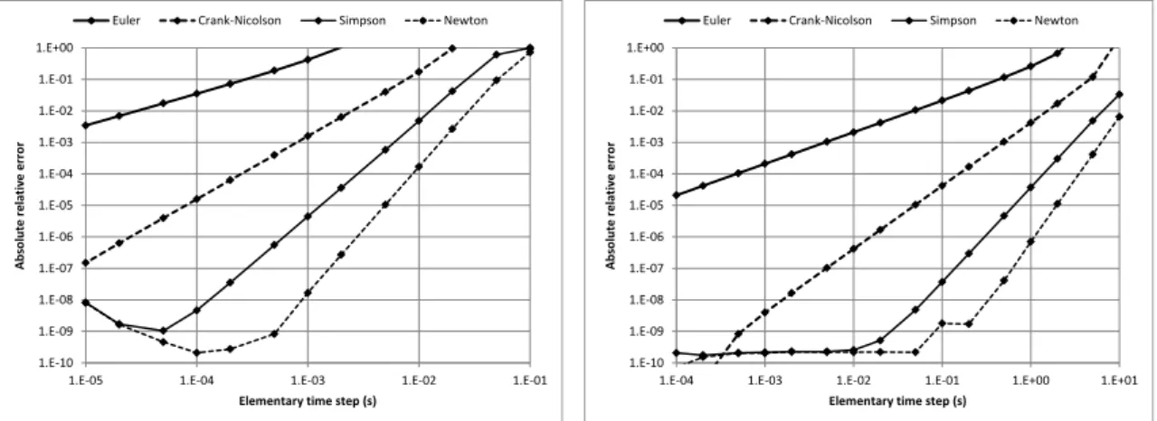
stable reference state, the control rod circled in Fig. 3 is instantaneously lifted by 35 cm, inserting a reactivity 𝜌 = 0.00301 < 𝛽. The transient is studied from 0 to 1 second. For this step insertion, the exact final value can be computed by matrix exponentiation. A PK step insertion of the same amount of reactivity is also simulated for comparison. The convergence behaviour of the 4 propagators used is given in Fig. 4 (absolute value of the relative error on the global amplitude with respect to the exact solution vs. elementary time step size). For this transient, the propagators of odd order (implicit Euler and Simpson) behave better than the even order ones (Crank-Nicolson and Newton).
Fig. 4. – 3-point MPK core test: step insertion. Kobayashi formulation (left), Avery formulation (right) 1.E-13 1.E-12 1.E-11 1.E-10 1.E-09 1.E-08 1.E-07 1.E-06 1.E-05 1.E-04 1.E-03 1.E-02 1.E-01 1.E+00
1.E-05 1.E-04 1.E-03 1.E-02 1.E-01 1.E+00
A b solut e r e lativ e e rr o r
Elementary time step (s)
Euler Crank-Nicolson Simpson Newton
1.E-13 1.E-12 1.E-11 1.E-10 1.E-09 1.E-08 1.E-07 1.E-06 1.E-05 1.E-04 1.E-03 1.E-02 1.E-01 1.E+00
1.E-05 1.E-04 1.E-03 1.E-02 1.E-01 1.E+00
A b solut e r e lativ e e rr o r
Elementary time step (s)
Page 23 sur 31
Computation times (Table 8) increase with the size of the problem, even if here, with 𝑁 = 3 and 𝐷 = 8, the sizes of the matrices involved remain modest: 9 × 9 (PK), 27 × 27 (MPK, Kobayashi) and 33 × 33 (MPK, Avery). Anyway, values exact to 5-8 places can be obtained using the Simpson propagator with a limited number of time steps, resulting in very short computation times (< 1s).
Table 8 – 3-point MPK core tests: computation times (µs per time step) for the finest time steps used
Approximate elementary propagator
Case Implicit Euler Nicolson Crank- Simpson Newton
Step PK 56 59 72 112 MPK (Kobayashi) 125 150 280 638 MPK (Avery) 167 196 355 954 Ramp PK 151 154 266 405 MPK (Kobayashi) 1470 1510 2997 4738 MPK (Avery) 4615 4632 9321 14550
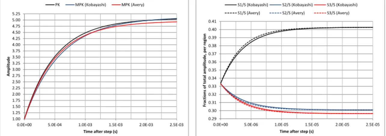
Starting from 1 at 𝑡 = 0, the amplitudes (= ∑𝑁𝑚=1𝑆𝑚) reached at 𝑡 = 1 s are very
similar; their 5-digit rounded values are 31.996 (PK), 33.483 (MPK, Kobayashi) and 31.317 (MPK, Avery). The time constant for the prompt jump in amplitude is (PK)
ℓ
𝜌−𝛽≈ −5.1 10−4 s for a jump by a factor
𝛽
𝛽−𝜌≈ 5.1; this is reflected by the plot given in
Fig. 5 (left). The relaxation time for the fission source distribution adjustment to the new asymmetric asymptotic distribution is expected to be of the order of a few generation times (ℓ ≈ 0.4 µs), the asymptotic shape being close to the static fission
source distribution (see 𝑆1 in Table 7). This is also confirmed by Fig. 5 (right).
Fig. 5. – 3-point MPK core test: step insertion. Prompt jump in amplitude (left) and shape adjustment (right) of the fission source distribution.
5.4. Application to a reactivity ramp test
1.00 1.25 1.50 1.75 2.00 2.25 2.50 2.75 3.00 3.25 3.50 3.75 4.00 4.25 4.50 4.75 5.00 5.25
0.0E+00 5.0E-04 1.0E-03 1.5E-03 2.0E-03 2.5E-03
A m p litu d e
Time after step (s)
PK MPK (Kobayashi) MPK (Avery) 0.29 0.30 0.31 0.32 0.33 0.34 0.35 0.36 0.37 0.38 0.39 0.40 0.41
0.0E+00 5.0E-06 1.0E-05 1.5E-05 2.0E-05 2.5E-05
Fr ac tion s o f to tal am p litu d e , p e r re gi o n
Time after step (s)
S1/S (Kobayashi) S2/S (Kobayashi) S3/S (Kobayashi) S1/S (Avery) S2/S (Avery) S3/S (Avery)
Page 24 sur 31
Here, starting from a stable reference state, the control rod circled in Fig. 3 is progressively lifted by 35 cm, inserting a reactivity 𝜌 = 0.00301 < 𝛽. The transient is studied from 0 to 1 second. In each of the three variants (PK, Kobayashi-MPK and Avery-MPK) all kinetic parameters and coupling coefficients are assumed to vary linearly with time between their initial and final values. This means that the transients do not represent the same physical scenario anymore, as for example the variations in time of the multiplication factor are no more the same. For the PK transient, the multiplication factor 𝑘 varies linearly in time; for the MPK transients it is the coupling matrix K that varies linearly in time, and no more the multiplication factor (the dominant eigenvalue of K). The variation laws of the multiplication factor are plotted in Fig. 6.
Fig. 6. – Variation law of the multiplication factor in the ramp tests (PK and 3-point MPK with Kobayashi’s and Avery’s models)
The global reactivity change from 𝑡 = 0 to 𝑡 = 1 s is given by the exact perturbation
formula Δ𝑘𝑒𝑥= <𝑆0
+,Δ𝐾 𝑆 1>
<𝑆0+,𝑆
1> ≈ 0.00302, whereas the first-order perturbation formula,
giving the slope of the 𝑘(𝑡) curve at 𝑡 = 0 is Δ𝑘1𝑜 =<𝑆0+,Δ𝐾 𝑆0>
<𝑆0+,𝑆0> ; this gives Δ𝑘1𝑜 ≈ 0.00247
with the Kobayashi K matrices, but only Δ𝑘1𝑜 ≈ 0.00057 with the Avery K matrices.
The convergence behaviour of the propagators used is given in Fig. 7. Having no external benchmark solution here, the reference used to compute the relative error is a Richardson extrapolated value for the Simpson propagator obtained for ∆𝑡 ∈
[10−4; 10−3], as in this elementary time step interval an asymptotic order 3 for the
Simpson propagator seems to be reached (see Fig. 7). For the Simpson and Newton propagators, the asymptotic order behaviour (order 3 or 4) is reached only for small elementary time steps and is at least partially masked by its subsequent degradation due to round-off error accumulation.
1.00000 1.00050 1.00100 1.00150 1.00200 1.00250 1.00300 0.0 0.1 0.2 0.3 0.4 0.5 0.6 0.7 0.8 0.9 1.0 M u ltipli cation fact o r Time (s) PK MPK (Kobayashi) MPK (Avery)
Page 25 sur 31
Fig. 7. – 3-point MPK core test: ramp insertion. Kobayashi formulation (left), Avery formulation (right)
Computation times per elementary time step are also given in Table 8. They increase noticeably with respect to the step reactivity insertion cases. However, the only difference between the step and the ramp cases is that in the step cases, the transition matrix step M is computed only once, whereas for the ramp cases M has to be computed 1 (Euler implicit and Crank-Nicolson), 2 (Simpson) or 3 (Newton) times per elementary time step. It is then supposed that the interpreted (slow) part of the code script, mainly devoted to fill in the matrix M at various time steps is the bottleneck with respect to computation time, as opposed to the compiled (fast) part devoted to matrix algebra, i.e. here mainly matrix products and inversions. Anyway, good accuracy (at least 5 digits on the final amplitude) can be obtained still with the Simpson or Newton propagators at limited time expense (< 1s).
Amplitudes and shapes are plotted in Fig. 8 and qualitatively match expectations: for final amplitudes, Avery MPK < Kobayashi MPK < PK due to the time law of reactivity insertion shown in Fig. 6; and there is a continuous shape adjustment to values close to the dominant eigenfunction of the current coupling matrix 𝐊(𝑡), due to very small generation times.
Fig. 8. – 3-point MPK core test: ramp insertion. Progressive adjustment in amplitude (left) and shape (right) of the fission source distribution.
6. Verification checks with SACRE
1.E-13 1.E-12 1.E-11 1.E-10 1.E-09 1.E-08 1.E-07 1.E-06 1.E-05 1.E-04 1.E-03 1.E-02 1.E-01 1.E+00
1.E-05 1.E-04 1.E-03 1.E-02 1.E-01 1.E+00
A b solut e r e lativ e e rr o r
Elementary time step (s)
Euler Crank-Nicolson Simpson Newton
1.E-13 1.E-12 1.E-11 1.E-10 1.E-09 1.E-08 1.E-07 1.E-06 1.E-05 1.E-04 1.E-03 1.E-02 1.E-01 1.E+00
1.E-05 1.E-04 1.E-03 1.E-02 1.E-01 1.E+00
A b solut e r e lativ e e rr o r
Elementary time step (s)
Euler Crank-Nicolson Simpson Newton
1.00 1.50 2.00 2.50 3.00 3.50 4.00 4.50 5.00 5.50 6.00 6.50 7.00 7.50 8.00 8.50 0.0 0.1 0.2 0.3 0.4 0.5 0.6 0.7 0.8 0.9 1.0 A m p litu d e
Time after step (s)
PK MPK (Kobayashi) MPK (Avery) 0.29 0.30 0.31 0.32 0.33 0.34 0.35 0.36 0.37 0.38 0.39 0.40 0.41 0.0 0.1 0.2 0.3 0.4 0.5 0.6 0.7 0.8 0.9 1.0 Fr ac tion s o f to tal am p litu d e , p e r re gi o n
Time after step (s)
S1/S (K) S2/S (K) S3/S (K) S1/S (A) S2/S (A) S3/S (A)