High dimentional neural fuzzy controller for nonlinear systems

UNIVERSITE DE

SHERBROOKE

Faculte de Genie

Departement de genie electrique et de genie informatique

HIGH DIMENSIONAL NEURAL FUZZY CONTROLLER

FOR NONLINEAR SYSTEMS

Memoire de maitrise es sciences appliquees

Speciality: genie electrique

Xiaodong Tan

1*1

Your file Votre reference ISBN: 978-0-494-49586-5 Our file Notre reference ISBN: 978-0-494-49586-5

NOTICE:

The author has granted a non-exclusive license allowing Library and Archives Canada to reproduce, publish, archive, preserve, conserve, communicate to the public by

telecommunication or on the Internet, loan, distribute and sell theses

worldwide, for commercial or non-commercial purposes, in microform, paper, electronic and/or any other formats.

AVIS:

L'auteur a accorde une licence non exclusive permettant a la Bibliotheque et Archives Canada de reproduire, publier, archiver,

sauvegarder, conserver, transmettre au public par telecommunication ou par I'lnternet, prefer, distribuer et vendre des theses partout dans le monde, a des fins commerciales ou autres, sur support microforme, papier, electronique et/ou autres formats.

The author retains copyright ownership and moral rights in this thesis. Neither the thesis nor substantial extracts from it may be printed or otherwise reproduced without the author's permission.

L'auteur conserve la propriete du droit d'auteur et des droits moraux qui protege cette these. Ni la these ni des extraits substantiels de celle-ci ne doivent etre imprimes ou autrement reproduits sans son autorisation.

In compliance with the Canadian Privacy Act some supporting forms may have been removed from this thesis.

While these forms may be included in the document page count,

their removal does not represent any loss of content from the thesis.

• * •

Conformement a la loi canadienne sur la protection de la vie privee, quelques formulaires secondaires ont ete enleves de cette these.

Bien que ces formulaires aient inclus dans la pagination, il n'y aura aucun contenu manquant.

RESUME

De nos jours, la theorie de controle joue un role significatif dans presque tous les domaine de la science et de l'ingenierie. Les controleurs lineaires PID sont les applications principales de la theorie de controle, et ils se basent sur les systemes de controle simples. Mais beaucoup de vrais systemes possedent des caracteristiques non-lineaires. Dans la pratique, il est necessaire de faire beaucoup de linearisations. Quand nous employons le controleur classique dans un systeme non-lineaire fortement complexe, les difficultes augmentent exponentiellement. Pour eviter les imperfections, on peut employer des controleurs flous. Le controleurs flous se basent sur le systeme de connaisance. Ce sont des outils importants dans le domaine de l'automatique. Ils possedent beaucoup plus d'avantages que les controleurs classiques "PID", mais ils ont besoin d'experts pour concevoir les regies de base. La limite principale des controleurs flous est la difficulte d'etablir les regies de base.

Maintenant, beaucoup de recherches sont consacrees a la fusion des reseaux de neurones et de systemes flous dans une nouvelle structure (les reseaux de neuro-floue). Cette approche combine les avantages de deux paradigmes puissants dans une capsule simple, et fournit un cadre puissant pour extraire des regies floues des donnees numeriques.

Cependant, cette technologie n'est pas parfaite. II reste quelques difficultes: beaucoup de regies floues sont necessaires, les algorithmes sont complexes et la fiabilite est basse (Par exemple, pour un meme modele ou fonction, les resultats dependent des ensembles d'apprentissage). Pour eviter les difficultes, ce memoire presente une nouvelle methode, appelee "inference neuro-floue de haute-dimension".

L'idee fondamentale de cette methode propose est de considerer chaque donne dans ce systeme comme point avec la haute dimension. Chaque dimension d'entree sera traitee en meme temps dans les memes sous-ensembles de haute dimension.

L'algorithme propose a ete examine sur differentes applications, et les resultats ont ete compares aux donnees editees sur trois problemes de repere.

Cet algorithme est simple a employer, et les resultats experimentaux prouvent que le nombre de faisceaux exiges est inferieur a ceux rapportes dans la litterature. L'exactitude de rendement est bonne dans beaucoup d'applications.

REMERCIEMENTS

Au terme de ce travail, je tiens tout d'abord a exprimer ma profonde gratitude a 1'endroit de mon directeur de recherche, le professeur et doyen au Faculte de genie du Universite de Sherbrooke Dr. Gerard Lachiver. Je le remercie aussi pour ses conseils et son support financier duree de ce projet.

Enfin, je remercie tout specialement ma femme wei He, pour leur soutien moral tout au long de ce travail, ainsi que mes parents et beaux-parents, wanhua tan, jiaping Lu, keyu He, et yufeng Xia, pour leur soutien et leur interet continus.

Encore une fois, Merci beaucoup, il n'y a aucun de mot qui peut exprimer ma gratitude.

TABLE OF CONTENTS

1. INTRODUCTION 3

2. ARTIFICIAL NEURAL NETWORKS 6

2.1 Artificial Neural Networks 6 2.1.1 Supervised learning 9 2.1.2 Unsupervised learning 13

2.1.3 Clustering 17

3 FUZZY LOGIC 18

3.1 Fuzzy sets and membership function 18 3.2 Linguistic variables and linguistic rules 20

3.3 Fuzzy system 21 3.4 Fuzzy control system 36

3.4.1 SISO AND MISO 37

3.4.2 MIMO 38

4 DESIGN OF A HIGH-DIMENSIONS NEURAL FUZZY CONTROLLERS

(HDFIN) FOR NONLINEAR SYSTEMS 40

4.1 High-dimensions fuzzy inference 41

4.2 Input space clustering 46 4.3 Membership function forming 47

4.4 Identification parameters matrix derivation for T-S fuzzy rules 48

4.5 Conclusion 49

5. RESULTS AND COMPARATIVE ANALYIS 50

5.1 Nonlinear function approximation 50 5.2 Mackey-Glass time series prediction 53 5.3 Nonlinear system control: the ball and beam example 57

7. APPENDIX A 68 8. APPENDIX B 71 9. BIBLIOGRAPHY 78

1. INTRODUCTION

Today, the control theory plays a significant role in almost every field of science and engineering. The classical theory of automatic control systems has been widely used in modern society and it ranges from simple application, such as in washing machine control systems, to highly sophisticated systems such as space shuttles, satellites and intelligent robots. Throughout the history of control, the goal has been to mimic the human worker interacting with machines and to process events without human interaction. In recent years, researchers work to design controllers that have the ability to "learn" and "think" like human expert [1] [2].

Fuzzy theory is a powerful problem-solving method with wide applications in industrial control and information processing [3] [4] [5]. It provides a simple way to draw definite conclusions from vague, ambiguous and imprecise information. Unlike classic approach which needs a deep understanding of system dynamics and the knowledge of exact equations and precise numerical values, fuzzy logic incorporates simple rule-based "IF X AND Y THEN Z" approach to solve control problem rather than trying to model it mathematically. Fuzzy modeling based on numerical data, which was first explored systematically by Takagi and Sugeno [6], has found many successful applications to complex system modeling. Fuzzy controllers are the most important application of the fuzzy theory. They work rather differently than conventional controllers by using expert knowledge (rules) instead of differential equations to describe a system. The knowledge could be expressed in a natural way with "linguistic variables", which are described by "fuzzy sets". Fuzzy logic has many advantages but also has some limitations. For example, fuzzy systems needs expert for rule discovery and they cannot learn the rules themselves.

Artificial Neural Network (ANN) is an important concept in artificial intelligence. These networks are based on the parallel architecture of human brain. The true power and advantage of neural networks lies in their ability to represent both linear and non-linear relationships and in their capacity to learn these relationships directly from training examples. The training examples must be selected carefully otherwise useful time is wasted or even worse the network might be functioning wrongly. ANN is made of many highly interconnected processing elements (neurons) working in unison to solve specific problems. It can create its own organisation or representation of the information it receives during learning time but the knowledge represented by the network is difficult to understand. Also, the mathematical theories used to guarantee the performance of an applied neural network are still under development.

Many researches are devoted to fusion of neural networks and fuzzy system into new structures called "Neuro Fuzzy Networks". These approaches combine the benefits of two powerful paradigms into a single capsule and provide a powerful framework to extract fuzzy rules from numerical data [7], [8], [9], [10], [11], [12]. Neuro fuzzy networks are widely used in many fields. In fact, a fuzzy system can be seen as a special neural network and represented as a three-layer feedforward network [13] [14]. However this technology is not perfect. Neuro fuzzy networks behave like "black boxes" whose internal rules of operation are unknown. Nodes and links in a neuro fuzzy network correspond to a specific component of a fuzzy system, some represent linguistic terms, some input or output variables and some are used for representing fuzzy rules. All nodes are not fully connected to the nodes in the neighboring layers. This arises several questions such as: how to optimize a neuro fuzzy network, how to set a large number of parameters, how to reduce convergence time and how to realize effective training and adaptation?

The aim of this work is to answer these questions by proposing a new clustering neuro fuzzy method. The objective is to improve the accuracy in modeling applications, and to reduce the number of fuzzy rules and to realize reliable adaptation in fuzzy control applications.

The method uses clustering techniques and Takagi-Sugeno modeling. The learning phase starts with a clustering algorithm which divides the input space into a series of clusters according to the input data distribution. These clusters are then used to construct a series of membership functions for the input space mapping. As a result, a collection of fuzzy sets represents all inputs. Finally an identification parameters matrix P is drawn by Takagi-Sugeno modeling and matrix operations. This matrix holds all identification parameters for the consequent part of the T-S fuzzy rules. In a certain extent, this matrix is equivalent to a rule base. After training, the matrix will be use to compute the system output. The main advantage of the proposed method is its simplicity, a fast convergence time and great accuracy.

This work is divided as follows: chapter 2 and chapter 3 introduce fuzzy logic and neural networks. They describe essential knowledge and information needed to design neuro fuzzy networks. In chapter 4, the proposed method is developed in details. Performances and results are evaluated and discussed for three different types of application in chapter 5: prediction, approximation, and control. Finally, conclusions are given in chapter 6.

2. ARTIFICIAL NEURAL NETWORKS

Neuro fuzzy systems have the structure of Artificial Neural Networks and the abilities of fuzzy inference. Therefore, a good understanding of ANN is important to design neuro fuzzy systems.

2.1 Artificial Neural Networks

ANN is an information processing paradigm inspired by our knowledge on biological nervous system. This idea was established before the arrival of computers. In 1943, a neurophysiologist Warren McCulloch and a young mathematician Walter Pitts wrote a paper on how neurons might work [15]. To do so, they modeled a simple neural network with electrical circuits. With computers, it is now possible to simulate more complex neural networks and to mimic human learning skill.

Neural networks try to reproduce the structure of neurons in the human brain. They are a powerful data-modeling tool. Knowledge in neural networks is stored within the synaptic weights like inter-neuron connection strengths. Neural networks have typically a multi-layer architecture where layers of nodes are connected [16].

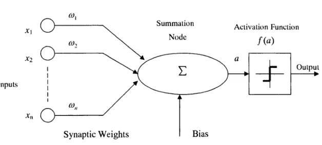
In a neural network, the basic element is the artificial neuron which is a device with several inputs and one output. Figure 2.1 shows the model of a single artificial neuron.

X\ X2 Inputs

Xn

O

Synaptic Weights Bias

Activation Function / ( « )

a

/ "

Output

Fig 2.1 Artificial Neuron Model

A single neuron, called a perceptron, is characterized by the parameters:

0 = (cot, o)2,...,con,b,f). (2-1)

Each connection link has a synaptic weight that multiplies the signal transmitted. Each neuron has an activation function being applied to the weighted sum of the inputs signal and the bias to produce an output signal y :

y = f

• n

yaw

The activation function can be a threshold function, a piecewise-linear function or a sigmoid function.

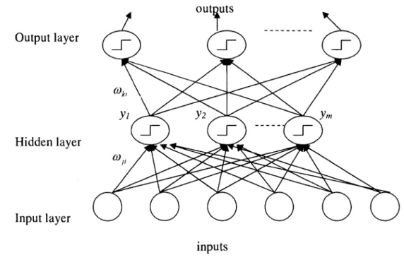
A multi-layer neural network is a neural network with more than one layer of neurons. In this case, the activation functions of the different neurons can be different. There are no connections between neurons of the same layer, only weighted connections with neurons in the next layer [16], [17]. Figure 2.2 shows a typical multi-layer neural network architecture.

By using proper input and output training samples, an ANN can learn to approximate complex relationships between inputs and outputs. Through the learning process, an ANN can be configured for a specific application, such as approximation, pattern recognition or data classification. However, the accuracy of the output is limited because the variables are effectively treated as analog variables, and the recursive least squares algorithm used during the learning process does not necessarily lead to a null error. Also, the needed time for proper training of a neural network can be long.

Output layer

Hidden layer

Input layer

inputs

Fig 2.2 Typical Neural Network Architecture

Neural networks need to be trained before they can be used. They improve their performances during the learning process. Learning occurs through an iterative process of adjustment applied to all weights and bias of the network. Learning methods used for neural networks can be classified into two main categories: supervised learning and unsupervised learning [18].

2.1.1 Supervised learning

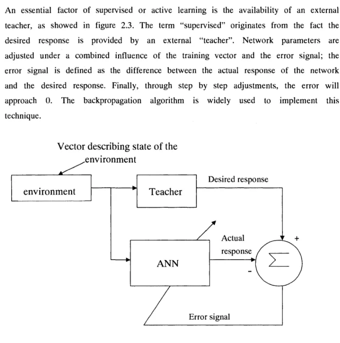
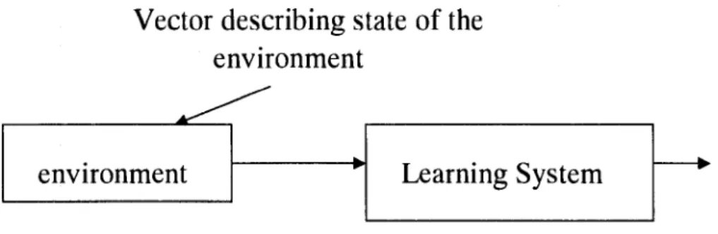
An essential factor of supervised or active learning is the availability of an external teacher, as showed in figure 2.3. The term "supervised" originates from the fact the desired response is provided by an external "teacher". Network parameters are adjusted under a combined influence of the training vector and the error signal; the error signal is defined as the difference between the actual response of the network and the desired response. Finally, through step by step adjustments, the error will approach 0. The backpropagation algorithm is widely used to implement this technique.

Vector describing state of the

..environment

environment

Desired response

Fig 2.3 Supervised Learning

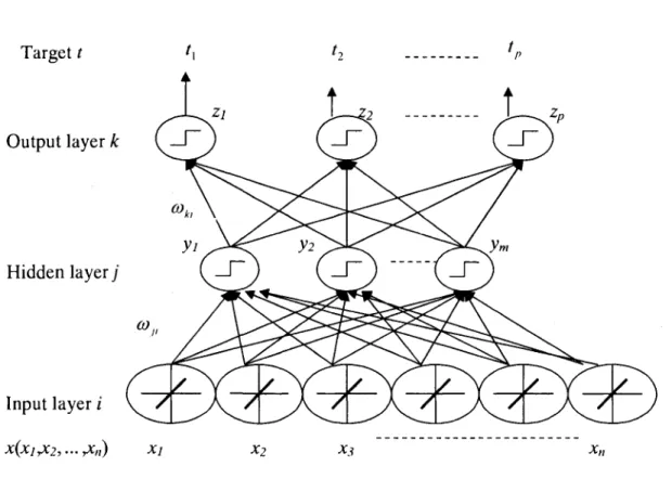
artificial neural networks. Standard backpropagation is a gradient descent algorithm, in which the network weights are moved along the negative of the gradient of a performance function. Properly trained backpropagation networks tend to give reasonable answers when presented with inputs that they have never seen before. In backpropagation, the output error on the training examples is used to adjust the network weights. Figure 2.4 shows a typical three layers network.

Target t Output layer k U Hidden layer; Input layer i X(XirX2, ••• yXn) Xl

Fig 2.4 Typical BackPropagation Network

Let tk be the £-th target (or desired) output, z* be the A:-th computed output with

k = 1,..., p and corepresents all the network weights andx the inputs. The training error is given by:

1 p

The backpropagation learning rule is based on gradient descent. The change in each weight vector component is proportional to the negative of its gradient:

Aa

=

-r

f (2-4)

Where rj is a constant called the learning rate chosen between 0 and 1.

a)(m +1) = co{m) + Aco(m) (2-5)

where in is the m-th pattern presented.

Backpropagation involves two passes. In the forward pass, the input signals propagate through the network to the output. In the reverse pass, the calculated error signals propagate backwards through the network where they are used to adjust all the weights. Calculating the output is carried out, layer by layer, in the forward direction. The output of one layer is the input to the next layer. In the reverse pass, using the delta rule, the error value of each output neuron guides the adjustment of the associated weights. Since the middle-layer neurons have no target values, the error must be propagated back through the network layer by layer [19].

Suppose netj is the inner product of the input layer signals with input weights for hidden unity:

n

net

=Y

°

v (

"

)

The hidden unit output is then computed:^ = /(netA, where / ( . ) is a nonlinear activation function. The error on the hidden-to-output weights is given by:

de de dnetk _ dnet,

~ ••• = Sk-T-jL (2-7)

where:

de _ de dzk

dnetk dzk dnetk

= (tk-zk)f'(ne(k) (2-8)

Suppose netk is the inner product of the input layer signals with input weights at the output unit k:

mtk=%y.,o>kj (2-9)

./ = !

On the output layer, the change in each weight vector component is:

A^ , = riSkyj = rj(tk -zk)f'(netk)yj (2-10) Equations for the hidden layer are the same as for the output layer except the error term must be generated without a target vector.

Error on the input-to-hidden units is given by:

de _ de dy t dnet, dcon dy} dnet] dm n (2-11) where: de "*y, d k = \ *yj p

= -E('*-

*)

(

'*H

t r

Jy, h

dnet

dy, (2-12)

* = i

According to (2-8) one can define:

<W'H>)I>*A

The learning rule for the input-to-hidden weights is:

A<y„ = i1xlSJ = r1{^jwkjdk)f'{net)xl (2-14)

Backpropagation technique summary [20]:

1. Randomize the weights to small random values (both positive and negative) to ensure the network is not saturated by large values of weights.

2. Select a training pair from the training set. 3. Apply the input vector to network input. 4. Calculate the network output.

5. Calculate the error, the difference between the network output and the desired output.

6. Adjust the weights of the network in a way that minimizes this error.

7. Repeat steps 2-8 for each pair of input-output vectors in the training set until the error for the entire system is acceptably low.

The training algorithm updates the parameters to match one input-output pair at a time. Others algorithms, such as recursive least squares, minimize the summation of the matching error for all the input-output pairs.

2.1.2 Unsupervised learning

In unsupervised or self-organized learning there is no external teacher or critic to oversee the learning process, as showed in figure 2.5. The word "unsupervised" means that no target values are needed. In fact, for most varieties of unsupervised learning, the targets are the same as the inputs. Unsupervised learning usually performs tasks like: classify data or compressing information from inputs. A typical unsupervised learning technique is competitive learning.

Vector describing state of the

environment

environment

Learning System

Fig 2.5: Unsupervised Learning

A basic competitive learning network has one layer of input neurons and one layer of output neurons (fig 2.6). An input pattern X is a sample point in the ^-dimensional real vector space (/?"). Competitive learning is an unsupervised learning paradigm, so it just extracts information from the input patterns alone without the need for a desired response. In a competitive-learning network, a neuron's synaptic weight vector typically represents a set of related data points, and is able to find the largest or smallest output. It associates those groups with one another and with a specific proper response. Normally, when competition for learning is in effect, only the weights belonging to the winning processing element will be updated. This element is called "winner" and is determined as the element with the largest weighted-sum Net?, where:

Net* = wjxk (2-15)

Where xk is the current input. Thus the iih element is the winning unit if:

w,rxk > w]xk for all j * i (2-16)

which may be written as:

The concept of choosing a winner is a fundamental issue in competitive learning. In general, the winner is the best output (depending on the criteria) and this system is called "winner-take-all" network. The simplest architecture is a single layer of units, each receiving the same input X^R" and producing an output Y. It is also assumed that only one unit is active at a given time see Figure 2.6.

y\

— •

yi

— •

" l r n

Fig 2.6: Single Layer Competitive Network

For a given input x* drawn from a random distribution p(x), the weights of the winning unit are updated (the weights of all other units are left unchanged) according to:

co,(t + l) = <y((t) + a(t)-(x(t) - a)j(O) if/is winner index (2-18)

o)l (t + 1) = <w,.(t) if / is not winner index (2-19)

Where a is a scalar called adaptation gain or step rate, 0 < « ( / ) < 1. The variable a controls how large the update's rate is at each step. If the step rate is close to 1, the network will converge quickly, but any new input can upset the cluster. On the other hand, if a is too small, the convergence will be too slow. A compromise is to use a variable step rate a(t) during learning. In general, there are three types of step

X\

*2

rate.

a. Constant learning rate

Suppose the learning rate is constant, so:

a(t) = a0 (2-20)

b. /C-means learning rate:

a{t) = - (2-21) m

Where the time parameter m stands for the number of input signals for which this particular unit has been winner so far.

c. Exponentially decaying learning rate

The exponential decay learning rate is given by:

a{t) = a,{—)'/,,m (2-22)

a,

Where al and af are the initial and final value of the learning rate, /11111X is

the total number of adaptation steps which is taken.

Every update strategy has its advantages and disadvantages: /C-means is simple, but " 1

the harmonic series lim V = oo diverges, so even after a large number of input signals and similarly low values of the learning rate arbitrarily large modifications of each input vector may occur. Constant learning rate has no convergence, but its practical effect is better than /C-means in many cases. Exponentially decaying learning rate has good effect than the two other strategies, but in many cases tmax is unknown.

2.1.3 Clustering

To fuzzify input signals in a fuzzy system, it is important to have a series of proper membership functions. Clustering technology is a good way to compose these membership functions. The key idea is to use clustering technology to class the input space into a series of subspaces, and then, to use cluster to construct membership function for each subspace.

Clustering is one of the most important unsupervised learning technologies. A loose definition of clustering is "the process of organizing objects into groups whose members are similar in some way". The goal of clustering is to reduce the amount of data by categorizing or grouping similar data items together. Such grouping is pervasive in the way humans process information, and one of the motivations for using clustering algorithms is to provide automated tools to help in forming categories or taxonomies [21] [22].

A cluster is a collection of objects which have similitudes between them and are "dissimilar" to the objects belonging to other clusters. Competitive rule allows a single-layer linear network to group and represent data samples that lie in a neighborhood of input space. Each neighborhood is represented by a single output neuron. From the view of the input space, clustering divides the space into local regions, each of which is associated with an output neuron. If the vectors are in the same cluster then they are similar. It usually means that they are "close" to one another in the input space. Clustering is a mechanism that changes a continuous space to a series of discrete vectors. If the number of clusters is enough, the error between a data sample in the neighborhood and its center is small, so the fidelity is high. However at present time there is no algorithm to find the optimal clusters for an input space.

3 FUZZY LOGIC

Lotfi Zadeh, professor at the University of California at Berkeley, first introduced fuzzy logic in the mid-1960's. Fuzzy logic is a powerful problem-solving theory with many applications in control engineering and information processing. Fuzzy logic provides a remarkably simple way to draw definite conclusions from vague, ambiguous or imprecise information. In a sense, fuzzy logic resembles human decision making with its ability to work from approximate data and find precise solutions. Fuzzy logic incorporates an alternative way of thinking which allows modeling complex systems using a higher level of abstraction originating from our knowledge and experience. Fuzzy Logic allows to expresse this knowledge with subjective concepts such as very well or bright red to be maped into exact numerical ranges [23] [24].

3.1 Fuzzy sets and membership function

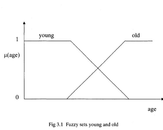
Fuzzy sets are extension sets of the classic sets. Fuzzy sets, unlike classic sets, have no crisp boundary, and they provide a gradual transition between "belonging to" and "not belonging to" a set. A fuzzy set in a universe of discourse X (which contains all the possible elements of concern in each particular context or application) is characterized by a membership function MA(X) that takes values in the interval [0, 1]. In other words, a fuzzy set is a generalization of a classical set by allowing the membership function to take any values in the interval [0, 1]. The fuzzy set theory makes it possible for an object or a case to belong to a set to a certain degree [25]. For instance, we might think that age 20 is "young" with membership value of 1. Age 30 has a membership value of 0.95. Age 60 has a membership value of 0.1, and so forth. That is to say, every people is "young" to a certain degree. Figure 3.1 describes a possible relationship between fuzzy sets "young" and "old".

1

H(age)

0

age

Curves in figure 3.1 are the membership function of the fuzzy set "young" and the fuzzy set "old". The membership value of each element is between 0 and 1. The values 0 and 1 describe "not belonging to" and "belonging to" a classic set respectively. Elements of a fuzzy set are taken from a universe of discourse, also called its universe. The universe contains all elements that can come into consideration. In general, fuzzy sets can either be discrete or continuous. For example, a fuzzy set A in universe X may be represented as a set of ordered pairs of a generic element x and its membership value, that is,

A = {(x,MA(x))\xeX} (3-1)

When X is a discrete set:

A

= y nM.

(3-3)

x X

Where the summation sign does not represent arithmetic addition; it denotes the collection of all points x e X with the associated membership function juA (x).

When X is a continuous and infinite set:

A

=

[A.

.

)

S x,

3.2 Linguistic variables and linguistic rules

Just like an algebraic variable takes numbers as values, linguistic variables take words or sentences as values. A linguistic variable is characterized by a quintuple

(X; T(X); U; G; M) in which X is the name of the variable, T(X) is the term set, U is a universe of discourse, G is a syntactic rule to create the elements of T(X) and M is a semantic rule for associating meaning with the linguistic values of X [6]. In figure 3.1, the "age" is a linguistic variable.

Fuzzy if-then rules (linguistic rules) or fuzzy conditional statements are expressions of the form if A then B, where A and B are labels of fuzzy sets characterized by appropriate membership functions. Inputs of a fuzzy system are associated with the premise, and outputs are associated with the consequence. Assume that a fuzzy system has m+k linguistic variables: m inputs xj, X2 ,x„, and k outputs yi, y2 , y* and that n linguistic rules defined by:

/?/.• ifxi is An andx2 is Kn and, ,andxm is Ajm

Then yi is Cu andy2 is C/2 and, ,andy^ is C;*

Then yi is C„i andyi is C,a and, ,andyk is C„*

3.3 Fuzzy system

Fuzzy systems have been applied to a wide variety of fields ranging from control, signal processing and communication. However, the most significant applications are in control problems. In general, a fuzzy system consists of four components: fuzzification, fuzzy inference, defuzzification and fuzzy rule base (Figure3.2). The function of fuzzification is to map a crisp input to a linguistic value. After fuzzification, the inference engine uses a fuzzy if-then rules base and linguistic values to form linguistic output. Once linguistic output is available, the defuzzification step produces a final crisp value from linguistic values.

crisp output

•

fuzzy rule base

Fig 3.2 Fuzzy System

3.3.1 Fuzzification

Fuzzification transforms crisp values x, into grades of membership for linguistic

crisp input

fuzzification

fuzzy

inference

i i

terms of fuzzy sets A,. The simplest form of fuzzification can be done using a fuzzifier function / that fixes the degree of fuzziness //(A,) in a set.

For example, suppose A, is the input space, xt is an input vector and xl e A,. The fuzzification performs to transform x, to every fuzzy set A, defined by function / :

/i(Af ) = / ( * , ) (3-3)

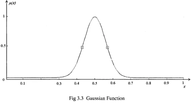
In general, Gaussian or triangular membership functions are used as fuzzifier.

A Gaussian function is defined by:

(x-a)2

ju(x) = exp(- — - y — )

2b (3-4)

Where a is the peak value and b is the width of the membership function (fig 3.3).

0.5

MM

o.i 0.3 0.4 0.5 0.6 0.7 0.8 0.9

Fig 3.3 Gaussian Function

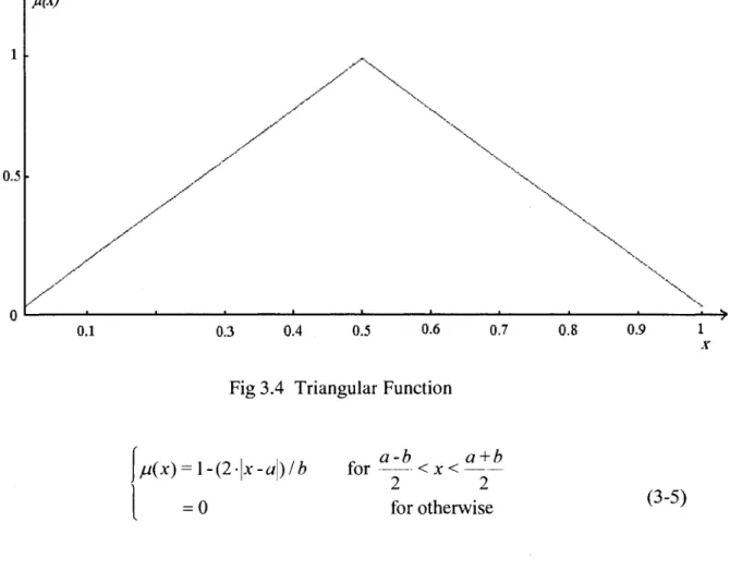
general form is (3-5): *M(x) IV y \ \ \ \ 0.5 / y / / v \ 0.1 0.3 0.4 0.5 0.6

Fig 3.4 Triangular Function

0.7 \ V 0.8 0.9 1 x ju(x) = l-(2-\x-a\) / b = 0 a-b a+b for < x < 2 2 for otherwise (3-5)

In triangular or Gaussian functions, there are two unknown parameters, center and width. In most case, the center points can be found by clustering technique, and the width factors can be determined by two ways.

a. Constant width

If the width is constant for all the membership functions, then the width can be defined by:

S = d i ^ (3-6) ,'2M

Where M is number of subsets, and d(max) is the maximum distance between those centers of subsets. This form would be close to the optimal solution if the data were uniformly distributed in the input space leading to a uniform distribution of the centers. Unfortunately, most real-life problems show non-uniform data distributions. The method is thus inadequate in practice and an identical width for all Gaussian kernels should be avoided since their widths should depend on the clusters position, which in turn depends on the data distribution in the input space.

b. Independent width

If the width of each Gaussian function is independent, the following form can be used to define the width of each function:

min{ ||V, - V,|j /, 1 = 1 , 2 , - , * i*L)

\ = (3-7) Where k is the number of subsets, V, and Vi are the center of subset, and i is not

equal L. In practice, another form, based on the r-nearest neighbor of the center is often used:

2 |

8L = - ^ (3-8)

Where the V,- are the r-nearest neighbors of center VL. A suggested value for r is 2k. The form (3-7) and (3-8) offer the advantage of taking the distribution variations of the data into account. In practice, they are able to perform much better as they offer a greater adaptability to the data than a fixed-width procedure.

3.3.2 Defuzzification

The outputs of a fuzzy system are fuzzy. They often need to be converted into a scalar. This process is called defuzzification. Defuzzification is especially necessary for hardware application because conventional systems work with crisp data exchange. However, selecting a single scalar value from a series of fuzzy outputs is a challenging task. There are many defuzzification methods: Centroid Average (CA), Maximum Center Average (MCA), Mean of Maximum (MOM), Smallest of Maximum (SOM) and Largest of Maximum (LOM) Centroid Average and Maximum Center Average methods belong to continuous methods and are frequently used in control engineering and process modeling. The rest represents discontinuous methods, which are mainly used in decision-making and pattern recognition applications. For convenience, we could divide all the defuzzification methods into two basic mechanisms: centroid and maxima. The centroid methods are based on finding a point within the total geometric figure such as the weight of each fuzzy set, the area of the largest fuzzy set, or the area of the highest intersection.

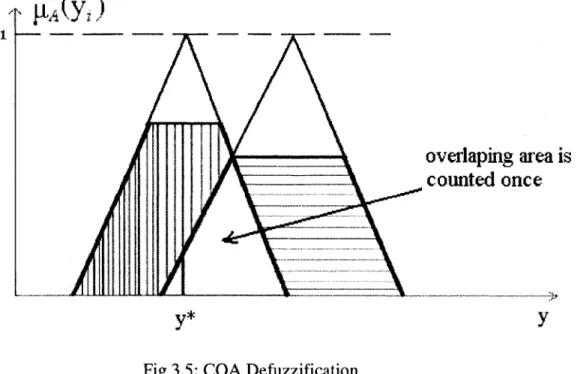
a. The Center of Area Defuzzification:

The Center of Area (COA) method is often referred to as the Center-of-Gravity because it calculates the centroid of the composite area representing the output fuzzy term (3-9). It specifies the crisp value y* as the center of the area covered by the membership function of fuzzy set A.

y* - - ^ — — - ( 3"9 )

L^M.Ay,)

The summation is carried overvalues of the universe of discourse y, sampled at N points. See figure 3.5.

t n*(y*)

overlaping area is

counted once

y* y

If we regard //,, (>»,•) as the probability density function of a random variable, then the center of area defuzzification gives the mean value of the random value. The advantage of COA lies in its intuitive likelihood. The disadvantage is the difficulty to calculate the summation in most real case since. COA favors "central" values in universe of discourse and that, because of its complexity, it may lead to rather slow inference cycles If the areas of two or more contributing rules overlap, the overlapping area is counted only once. This defuzzification method is often used [26] [27].

b. The center of sums defuzzification

The Center of Sums (COS) method builds the resulting membership function by taking the sum of output from each contributing rule. So, this sum is not just the union. The overlapping areas are counted more than once. This method can be carried out easily and leads to rather fast inference cycles and it is the most commonly used defuzzification method.

y * = (3-10)

Where ^ ( y , ) is the membership function which is at point y,- of the universe of discourse resulting from the firing of the kth rules (figure 3.6).

h

^ ( y

)

overlaping area is

counted twice

Fig 3.6 COS Defuzzification

c. The Mean of Maxima method:

The Mean of Maxima method (MOM) a simple method for doing the defuzzification. The output takes the crisp value of the highest degree of membership in ^ ( y , ) . If a system has more than one element in the universe of discourse having the same maximum value, a random selection can be used or a mean value is performed. Suppose, there are M such maxima in a discrete universe of discourse. The crisp output can be obtained by:

y * = (3-11)

Where ym is the mth element in the universe of discourse where the membership function of /^(y,) is at the maximum value, and M is the total number of such elements. MOM defuzzification is faster than COA. Furthermore, it allows the controller to reach values near the edges of the universe of discourse. This method does not consider the overall shape of the fuzzy output //^(y,) (fig 3.7).

t^>Y)

Fuzzy value with

maximum height

3.3.3 Fuzzy Inference

Fig 3.7 MOM Defuzzification

To draw conclusions from a rule base, a mechanism that can produce an output from a collection of If-then rules is necessary. This mechanism is called fuzzy inference. There are two major inference methods: T-S fuzzy inference and Mamdani fuzzy

inference. The Mamdani fuzzy inference method is the most common method.

a. Mamdani fuzzy inference:

The Mamdani method was proposed in 1975 [28], to control a steam engine and boiler combination. In this application, the set of fuzzy rules was supplied by experienced human operators.

The following example is a typical Mamdani fuzzy rule.

Rj.- ifxi is An and %2 is Ai2 and and xr is A,> then y is C, (3-12)

Where Rt is the /' fuzzy rule; x is an input and A is a fuzzy set. The following two examples explain the Mamdani fuzzy inference.

Single fuzzy rule

If A: is A then}' is C If x is A' then C is? C'=min{C, max(A,A')} M P fi M M y

c=?

MriiL

Multiple fuzzy rules Rulel: If x is A; theny is C; *" y Rule2: If x is A2 theny is C2 _M

jm&.

C"=miiUCi. maxfAi. A'H+ min/Ci. maxfA?. A'H

0

y

C

/ ^ .

y Fig 3.9 Multiple Fuzzy Rules of Mamdani Method

b. Takagi-Sugeno fuzzy inference

The Takagi-Sugeno fuzzy inference method was introduced in 1984 and it is similar to the Mamdani method. The first two parts of the fuzzy inference process, inputs fuzzification and fuzzy operators, are the same. The main difference between Mamdani and Sugeno is Takagi-Surgeon approximates a nonlinear system by a combination of several linear systems (see figure 3.10). It breaks down the input space into several subspaces and represents the input/output relation in each subspace by a linear equation. A typical model of Takagi-Sugeno fuzzy inference is:

If input x = Ai and input y =Bj, then output is z = ax + by + c.

Where a, b, c are numerical constants.

y A

;

s

->

x

Fig 3.10 Linear approximation by 3 fuzzy rules In general, Takagi-Sugeno rules have the following form:

If xj isAu, and ... andxr isAir then y' - fj(x,,x2,---,xr)= b' +a[xi + —t-a'mxm (3-14) Where fi is the linear function, a and b are parameters of this linear function, _y, is the inference consequence of this rule.

T-S method can be easily represented and evaluated by a three-layers' neural network. Let us suppose a multiinput system with n inputs D(x{, x2, x3, x4, ..., xn) and an output Y(_y,, y2, y3, y4, ..., yk) (figure3.11).

X\ Xi D = (x,,x2,...,*„)\J Layer 1 Fuzzification Layer 2 Product Operator Layer 3 Defuzzification

Fig 3.11 Takagi-Sugeno Fuzzy System

Layer 1:

The nodes of first layer receive input vector D(x,, x2, x,, x4, ..., xn) and act as fuzzy sets representing the terms of the matching input variable. Nodes in this layer are arranged into n groups; each group representing the (/"-part of fuzzy rule. Each node acts as a fuzzifier. Hence, the node outputs are in the range [0, 1] and are calculated by the following function:

Layer 2:

The number of nodes in this layer is equal to the number of fuzzy rules. A node in this layer represents a fuzzy rule. Each node in this layer is a product operator. The "min" operator is not used, because the function "min" is not differentiable in the set of real numbers iR. Outputs of this node are:

<0\ = Mu Oi) th, (*2)' •' Mm, (*».) 0 ^ ' ^ <l) (3-16)

= rW*<> (

3

-

17

)

7=1

co is called the firing strength. Layer 3:

Nodes in this layer represent the output variables of the system. Each node acts as a defuzzifier. Outputs of this node are:

y-^-.y'*^-y*-*^-y (3-18)

i<=\

•"I (3-19)

" II

The firing strengths a>, are normalised and outputs y are the crisp output sets weighted by the firing strengths.

A fuzzy rule (3-14) has four basic elements: input (JC, , x,, x,, JC4 ...,*„), input

space (All,A'2,---,A'm), output y and parameters of consequence (b',a\,---,a'm). In certain degree, the object of training is to draw the parameters of consequence, so

the following contents will introduce how to draw the parameters of consequence matrix P.

Suppose that we have n rules R' (/ = 1,2, •••,«) of the form:

R': IFx; isA/ and*2 i s ^ ' and...andx„, isA„', theny'=b'+ai'xi+a2lX2+ ... +a„,'xm If we apply the j"' sample to the i'h rule R', we obtain:

R/: IFxij isA\j andx2; isA2/ and...andx„y isAm/, Then yf=bl+a\'xij+ci2lX2j+... +am'xmj Where i=l,2,...,n andy=/,2,...,r.

So the weights of the rules are:

w) =xjj is Ajj and X2j is A2/ and... and xmj is Amf

= fl^K;) k=l,2,...,m (3-21)

According to (3-19), the output yy is given by:

y = ^1 Si n

i>;

= Z « (3-22)

i>;

yj=[A,02j-0„]

=[A,A,--A,]

So, the vector of output Y can be expressed by:

Y =

V

\Pu

Pa

A

-

A „ l

- P

_

••

l

i i "

We can rewrite in the form:

Where: Y = X P (3-26) Y = y\ yr (3-27) X = P l l ' * ' A i l ' X\\P\\ ' " X\\Pn\ '" Xm\P\\ '" Xm\Pn\ Pxr ••• A ,r> * 1 , A ••• XirPnr - *„„ A " • *r ar A . (3-28)

b"

p= (3-29)

X is a vector matrix with r x n(m +1) dimensions, Y is a vector with r dimensions,

P is a vector with nx(m + l) dimensions. Finally, vector P is expressed by:

P = [X^l'^Y

3.4 Fuzzy control system

Control systems are classified in two categories: open loop control systems, in which the control action is independent of physical system output, and closed loop system, also known as feedback control systems. The physical system under control is called a plant. In a closed loop system, a sensor measures the output signal and returns it to the input signal. To guarantee satisfactory responses and performance, it is necessary to use an additional system, known as a controller or a compensator into the loop. Currently, most controllers are based on proportional integral derivative (PID) technology. PID controllers work well in many control applications. But in practice, the system to control always contains uncertainty, is complex, poorly understood, or nonlinear. So it is difficult to build a precise mathematic model and is difficult to linearize. A fuzzy controller unlike a PID controller which needs a deep understanding of the system, exact equations and precise numerical values, uses a simple, rule-based if x AND v then z approach rather than trying to model a system mathematically. Fuzzy logic provides an alternative solution for nonlinear

applications. Fuzzy inference processes results in improved performance, simpler implementation, and reduced design costs. In many applications, fuzzy logic can lead to better control performances than linear, piecewise linear, or lookup table techniques. Most control applications have multiple inputs and require modeling and tuning of many parameters which makes implementation tedious and time-consuming. Fuzzy rules can help to simplify implementation by combining multiple inputs into single if-then statements while still handling nonlinearity.

In general, a fuzzy control system includes three major classes: single input single output (SISO), multi-input single output (MISO), and multi-input multi-output (MIMO).

3.4.1 SISO AND MISO

The "SISO" fuzzy controller is widely applied in practice. This class of controllers is simple (Fig 3.12).

Fig 3.12 Structure of a SISO

However, for dynamic systems, it is better to track also the trend of the error's change as shown in (Fig 3.13).

Fig 3.13 Structure of a MISO with differential input 3.4.2 MIMO

The design of controllers for MIMO systems has always been a hard problem even for the linear ones. Currently, there is no complete theory to design MIMO systems. Most of existed techniques are quite complicated. The main difficulties is the derivation of rules is not easy and the number of rules is too high, however it is possible to describe a "MIMO" system (figure 3.14) with several "MISO" systems (figure 3.15).

u(kt)

plant

yi(to)

y„(kt)

r(kt) / „ > «

AV

s~

--A^r

_{v ^}

4 DESIGN OF A HIGH-DIMENSIONS NEURAL FUZZY CONTROLLERS FOR NONLINEAR SYSTEMS

Fuzzy controller are widely applied and fuzzy systems have been proved to be able to approximate nonlinear functions with arbitrary accuracy [29] [30]. Generally speaking, fuzzy systems and neural networks have much equivalence [31] [32]. In fact, fuzzy control systems can be regard as special neural networks control systems and many neural networks learning algorithms can be used in fuzzy control systems. Neural fuzzy systems have good capacity for approximations; however, there are still some difficulties.

Many fuzzy rules are needed, which leads to excessive training time, particularly with multidimensional input.

* Algorithms are complex and problem adapted.

. The reliability is low. For example, for a same model or function, the learning results are dependent on the training sets.

To solve these problems, Jian-qin Chen and Yu-Geng Xi [33] developed a learning method. The basic idea is to use competitive learning for partition the input space to fix the decision boundaries for local regions in an input space, and then to learn the consequent part of the fuzzy rules by RLS (Recursive Least Square). In this method, the boundaries decision is an important step. The choice of decision boundaries is useful for dealing with the conflict between over fitting and generalization as well as reducing the number of local input regions in certain degree. The following section describes the decision boundaries algorithm:

Step 1. Freeze the cluster centers v, (i=l,2,... ,cluster_number). Step 2. Let r,=0 (i=l,2,..., clusterjiumber) at first

Step 3. For any input x(t) find out vc by

Step 4. Update rc

if |JC(/) —vt.| > rt., then rc(k + 1) = jpt(/)-v .;| (4-2) if ! j x ( 0 - v j < r . , then rc(k + l) = rc(k) (4-3) Where v, is the i'h cluster and r, is the radius of the local regions which center is v,.

The algorithm for determination of decision boundaries is efficient and simple. However in practice, this algorithm has some drawbacks. For example; two very closed points A and B, with similar characteristics, can belong to different clusters ("A" belongs to cluster N and M. "B" belongs to cluster M and P). This may lead to output errors (called boundary error). To decrease this type of errors and to improve the precision, it is necessary to increase the number of clusters and to lessen theirs radiuses. This method needs many clusters to guarantee a good accuracy.

X"

X / \ X '

X

x /

. / ^

X

X X

"

x

^i

x^ j*

X

x

>x

>' x

/x

A

<: x J ^ / x

\

x x

.-'''

x x

""""'

Fig 4.1 Boundary error during a clustering process

4.1 High-dimensions neural fuzzy inference (HDNFI)

To solve the problem mentioned above, in inference phase, a high-dimension neural fuzzy inference (HDNFI) which based on T-S model is proposed in this work (see figure 4.2)

,'X\ \ i X2

H

y

Fuzzification Inference and Defuzzification

Fig 4.2 High-dimension fuzzy inference

The basic idea of this method is to consider each data in this system as a point with high-dimension. Each dimension of input D will be processed at same time in same high-dimension subsets.

Layer 1:

The nodes of first layer receive input vector D(x,, x>, x3, x4, ..., jcn) and each node

acts as a fuzzifier. Therefore, the node outputs are in the range [0, 1] and are calculated by the following function:

//,(D) = exp-

™J^- (4-4)

2b-Where c, is the center and bt is the width of membership function (4-4), c, and D has same dimensions.

Layer 2:

This layer includes fuzzy inference and defuzzification. In this layer, the variable //, is the degree of fuzziness of input D in subset A, and suppose the firing strength cot equal to //,. The ouput is given by:

y=^- y+^-y+• • • + ^ r - y (

-

>

_i>y

=S'-,^

I" «,

Firing strengths a>l are normalised and outputs y are the crisp output sets weighted by the firing strengths.

Suppose that we have q rules R' (/ = 1,2,•••,#) of the form: R': If input D is in Aj then output is z' = a ' x D + 6' If we apply the /* sample to the i'h rule i?', we get:

R\: If input D, is in A, then output is z' = a / x D7 + V

Where i=l,2,...,q and j=1,2,...,r.

Where :

2»;

2>;

i«

The output y, can be expressed by:

yj=[AjAr~P

]

-[bj&j-PA

So, the vector of output Y can be expressed by:

Y =

V

\Pu

Pn

A

•

P*

}

V

"

U[

1

We can rewrite in the form

Where: yr (4-13)

x=

X is a matrix with r x q{n + 1) dimensions, Y is a matrix with r dimensions,

P is a matrix with q(n +1) dimensions. Finally, matrix P is expressed by:

'/i

P\r ••• Par, XUPU. ••• XlfB ••• Xmpu ••• XmPl

(4-14)

(4-15)

P = [XTX]"]XTY (4-16)

Obviously, in this method, the number of fuzzy rules is equal to the number of subsets (number of membership functions) and input D is processed by every membership function during the inference phase, that is to say input D is the member of all subsets, there is no step for choosing subsets. So, there is no boundary error. The points A and B in figure 4.1 will give similar output

if using the proposed method and this result is more reasonable than [33]. In this method, the characteristics of input data will be represented more accurately by those membership functions. The output accuracy will be improved. In other word, for a certain requirement of accuracy, this method can decrease the number of membership functions.

The following section presents the design process. Appendices A and B provide the detail flow chart and pseudo-code.

4.2 Input space clustering

A typical input space may contain a large number of inputs. But, it is not necessary to deal with each input. They can be grouped according to their common characteristics and then be represented by a point. This process is called clustering and this chosen point is called a cluster. Clusters can be multi-dimensional points, and competitive learning is often used to perform the clustering. The following algorithm is used for clustering.

Step 1. Fix the cluster number "clusterjiumber", initialize these clusters cluster (i) (/' = 1, 2, ••• , cluster number).

Step 2. By using a traditional learning algorithm to decide a winner, dead units (clusters which are never updated) may appear. To solve this problem, the following algorithm is used [33].

Pwmna-l XU)' duster (winner ID) \ = minpl( time_win(i)x.\ x(j)- cluste(i)\) (4-17)

w h e r e /,(= . _ 4 _ _ (4-18)

Where the cluster (winner_ID) (winner_ID=l,2,..., clusterjiumber) is the nearest cluster of x(j) and x(j) is the /h input of training sample, p, is roughly

equal to the probability of input data near the cluster (/), nt is the number of cluster(j') being chosen as a winner and m is the number of cluster [33]. The variable probability p is used to avoid dead units. So every cluster has a chance to competition.

Step 3. Update the cluster(win_ID) according to x(t) by:

tiuster(winlD) = cluster{winJD) + steprate x (x(j) - cluster{win_ID)) (4-19)

Where x(j) is the input vector ( j = \, 2, •••, numberJnput). The variable step_rate is used to avoid oscillation during the training time.

Step 4. Update step_rate (2-20)

a(t) = a,{aL)'""" (4-20)

«,

In general, it is difficult to know the exact value of each / v, but it can be

roughly set as the maximum number of iterations. 4.3 Membership function forming

At the end of the preceding section, the input space clustering is done. That is to say all the centers of the membership functions are fixed. However, just having centers is not enough to compose membership functions. It is necessary to find another parameter such as the width to describe each membership function. If the input space is uniformly distributed, then width can be inferred by equation (3-6). This method is simple and rapid. However if the input space is not uniformly distributed, then we need to use the independent width method (3-7) or (3-8) as following.

distance = m\n{\cluster{i)-cluster (b)\) (4-21)

Step 2. Calculate out widths by:

. , , distance .. . . .

width = (4-22)

4.4 Identification parameters matrix derivation for T-S fuzzy rules

In this proposed neural fuzzy system, the purpose of training process is to get an identification matrix P. This matrix contains all the identification parameters of consequent part of T-S fuzzy rules. It can be gained by the matrix operation (4-12) (4-13) (4-14) (4-15) (4-16). Matrix P is the core of the proposed controller. To get a desired output, a simple multiplication between fuzzy input and matrix P is performed.

Step 1. Fuzzification by Gaussian function or the triangular function (3-4) or (3-5)

dis = x(i)-cluster(j) (4-23) -ll/S

u{j,i) = e ^ ^ (4-24)

Step 2. Calculate P with equation (4-9)

Step 3. Use fi to construct input matrix X (4-14) Step 4. Calculate matrix P with equation (4-16)

Step 5. Calculate the final output with equation (4-12). If the final error is more than the expected error, then increase the number of clusters and retrains the controller.

dis is the distance between given input and a cluster. x(i) is the input vector (/ = 1, 2, • • • , m). "m" is the total number of inputs.

4.5 Conclusion

This method has three main parts. The first part is a competitive learning phase used to cluster the input space. Exponentially decaying learning rate is used in this phase, which can avoid oscillations during the training time. The second part forms membership functions. Independent widths are used to make membership functions more suitable for the input space. The third part is based on fuzzy inference and matrix operations to draw the identification parameters matrix P. This method has been validated on three different benchmarking problems and results are presented in the next chapter.

5. RESULTS AND COMPARATIVE ANALYIS

The validity of the proposed procedure has been validated by means of extensive computer simulations on three benchmark problems commonly used in the literature:

• Nonlinear function approximation. • Mackey-Glass time series prediction. • Nonlinear system control.

5.1 Nonlinear function approximation

Let us suppose a nonlinear system with a single output variable [34] [35] whose model is given by:

vfr 11)- MQyfr-i)yQ-2)"fr-iM-2)-i]+"(Q}

ll + yi(t-l)+yi(t-2)\

In this nonlinear function, the output value depends on its previous values y(t), y(t-1), y(t-2) and input values u(t), u{t-\). So, to approximate this function, a 5 dimension input vector x is defined where: x(t) = [u(t),u(t-\),y(t),y(t-\),y(t-2)] and an output y as a single dimension vector [_y(/ + l)]. This classic nonlinear function is often used to test the performances of fuzzy systems to approximate nonlinear functions.

Suppose u(t) = 0 and y(t) = 0 for ( s 0 . The learning procedure randomly generates input signal u(t) uniformly distributed in the range [-1, 1]. Using equation (5-1), the corresponding output y(t +1) is computed, thus composing the training samples

{x(t),y(t + \)}.

Then the training samples train the proposed neural fuzzy system using the following parameters:

Initial cluster number = 1; Initial update rate = 0.1;

Final update rate = 0.001. An exponential decay update strategy is used as given by equation (2-20);

Independent membership function widths (equation 3-7) are used;

If the final output error is more than 0.0001, increase cluster number by 1 and retrain the system.

Once the training is completed, the fuzzy inference system is tested with a new input given by:

«(0 = s i n - — for t<500 and M(0 = 0 . 8 s i n — + 0.2 s i n — - for t>500. (5-2) 250 250 25

The following figures show the resulting performances. Real output and expected output curves are shown in figure 5.1. As observed, these two curves almost completely overlap. The computed difference between the two outputs, called approximation error is illustrated in figure 5.2.

100 200 300 400 500 600 700 800

x 10

A

Ui

ft

A

w\/. \m

_u

u

Figure5.2: Approximation error.

Several authors have reported on the same experiment [33] [36]. To compare results with them, the same performance index as in [58] is used. Let's defined:

r'-itw-yQ]

i=i

In [33], the author used 50 clusters. The best case reported gives PI = 0.0012, the worst case PI = 0.0052 and the average case PI = 0.0029. In [36], the performance index is only 0.0052 when the author tests the generalization and he reported a PI = 0.00028 only when the training sets are chosen to be the same as the testing sets in which the generalization is ignored.

With the method described in this work, with 50 clusters used, the best performance index obtained is PI = 0.00008 and the worst case is PI = 0.0015. The average case is PI = 0.000308. This experiment shows that the proposed method is more accurate than those found in the literature and has good generalization properties.

5.2 Mackey-Glass time series prediction

The prediction of time-series is an important practical problem with applications found in economics, business planning, inventory and production control, weather forecasting, signal processing, and control. In this experiment, the proposed method is used to predict a Mackey-Glass chaotic time series [37]. This time series is created with the use of the Mackey-Glass time-delay differential equation defined here:

dx(t) = Olxit^

dt 1 + Jt'V-r) W V '

This time series, originally developed to model white blood cell production, is commonly used to test the performance of neural networks. This extremely chaotic series makes it an ideal representation of nonlinear oscillations found in many physiological processes. It has no obvious time period, is neither convergent nor divergent and its value at any time may depend on its entire previous history.

When JC(0) = 1.2, r = 17, this series is a non-periodic, non-convergent time series and is very sensitive to initial condition (x(t) = 0 for t<0). So in this experiment, JC(0) —1.2 and r = 17 has been used as initial conditions. The word prediction means that at time / the function value is known and the object is to predict the value at future time t + p. The standard method for this type of prediction is to create a mapping from D sample data points, sampled every A units in time, (x(t-(D-\)A,...,x(t-A),Jt(7)), to a predicted future value x(t + p). To compare with other articles [33] [38] [39] [40] [41], the conventional settings D = 4 and

A = p = 6 are used in this experiment.

A four dimensional input vector is defined in the following form:

A one dimensional prediction vector is defined in the following form:

output(t) = JC(/ + 6) (5-6)

A MATLAB demo called "Time-Series prediction" illustrates a Mackey-Glass series. This demo was used to generate training samples and test samples for the experiment. The samples was saved in a file mgdata.dat with (JC(0) = 1.2, r = 17). The following MATLAB program is used:

load mgdata.dat t = mgdata(:,l); x = mgdata(:,2); plot(t,x); for t=l 18:1117, Data(t-117,:) = [x(t-18) x(t-12) x(t-6) x(t) x(t+6)]; end

trnData = Data(l:500,:); % first 500 data pairs used to construct training samples. chkData = Data(501:end,:); % last 500 data pairs used to construct test samples.

In this program, the time range t is 118 to 1117 to be able to compare with results published by other authors. The trnData and chkData are 5-dimension arrays. The matrix trnData holds 500 training pairs, and matrix chkData holds 500 test pairs. The first four-dimension of trnData and chkData are used to construct training and test input vectors and the last dimensions of trnData and chkData are used to construct the training and test output vector.

The proposed neural fuzzy system was trained with the following parameters: Initial cluster number = 1;

Initial update rate = 0.1;

Final update rate = 0.001. An exponential decay update strategy is used as given by equation (2-20);

Independent membership function width (equation 3-7);

If the final output error is greater than 0.0001, increase cluster number by 1 and retrain the system.

Figure 5.3 gives the prediction error while figure 5.4 shows the computed output and the expected output in the same coordinate system. The difference is so small that it is almost impossible to distinguish the two curves.

618 668 718 768 818 868 918 968 1018 1068 1117

Fig 5.3 Prediction error.

8 668 718 768 818 868 918 968 1018 1068 1117