HAL Id: hal-02959434
https://hal.laas.fr/hal-02959434
Submitted on 6 Oct 2020
HAL is a multi-disciplinary open access
archive for the deposit and dissemination of
sci-entific research documents, whether they are
pub-lished or not. The documents may come from
teaching and research institutions in France or
abroad, or from public or private research centers.
L’archive ouverte pluridisciplinaire HAL, est
destinée au dépôt et à la diffusion de documents
scientifiques de niveau recherche, publiés ou non,
émanant des établissements d’enseignement et de
recherche français ou étrangers, des laboratoires
publics ou privés.
Saqib Amin, Usman Zabit, Olivier Bernal, Tassadaq Hussain
To cite this version:
Saqib Amin, Usman Zabit, Olivier Bernal, Tassadaq Hussain.
High Resolution Laser
Self-Mixing Displacement Sensor Under Large Variation in Optical Feedback and Speckle.
IEEE
Sensors Journal, Institute of Electrical and Electronics Engineers, 2020, 20 (16), pp.9140-9147.
�10.1109/JSEN.2020.2988851�. �hal-02959434�
redistribution to servers or lists, or reuse of any copyrighted components of this work in other works.
Abstract— Self-Mixing interferometry (SMI) signal characteristics are highly dependent on both the operating optical regime and
target surface. In this paper, a method is proposed to overcome some identified limitations of the even power scalable algorithm (EPSA) [1], such as the required operating regime to be weak feedback. In addition, by using the up-sampling techniques, the number of stages involved in the even-power scalable algorithm can be drastically increased without any data acquisition bandwidth modification. Here, 10 successive stages have been successfully implemented to achieve a theoretical resolution of λ0/213. It is further shown that the proposed method can handle and process weak, moderate and strong feedback regime as well as speckle affected SMI signals more efficiently. Lastly, FPGA based hardware emulation of EPSA is also done for later embedded implementation of this high-resolution algorithm. FPGA synthesis results show that the designed system can measure maximum target velocity up to 1.18 m/s while consuming total power of 1.4W.
Index Terms—Self-mixing, Signal processing, Speckle
I. INTRODUCTION
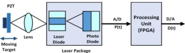
aser feedback based self-mixing interferometry (SMI) [2, 3] has been demonstrated for multiple sensing applications such as velocity [4], displacement [5, 6], distance [7], vibration [8], flow [9], tomography [10], 3D imaging [11], angle [6], and refractive index [12] etc. As opposed to conventional two-beam interferometry, SMI enables a compact, self-aligned and low-cost metric sensor (see Fig. 1).
In typical SMI setup, each interferometric fringe is assumed to correspond to remote target’s motion of λ0/2, where λ0 is the
laser’s wavelength. λ0/2 is thus considered basic resolution of
SMI sensors [2, 3]. However, many applications require much higher resolution than just λ0/2. E.g., in fabrication process of
lens surface element, measurements involving better than λ0/10
resolution are needed [13]. Similarly, nano-step height measurement in tomography [14] and surface imaging require nanometric resolution [15]. So, various methods are reported in literature to improve SMI resolution.
Using two reflectors, method capable of improving measurement resolution by 17 times was proposed [16]. However, the setup needed special arrangements to obtain partial reflection of signals from remote target, which is difficult to achieve during real-time measurements.
An external reflecting mirror was used to acquire λ0/6 fringe
precision [17]. However, due to use of external mirror, overall system becomes complex and costly. Furthermore, system requires angle measurements between target and external mirror, which is difficult to measure accurately, hence increasing chances of error in measurements. This system of [17] was improved by using the effect of orthogonal
polarization feedback to achieve resolution of λ0/58 [18].
Although measurement results for nanometer resolution were good, but performance of the system reduces when the reflection time goes up to 29 times.
A digital closed-loop vibrometer [19] using fringe-locking [20] was proposed for nanometric sensing. However, the achievable precision and dynamic range are limited by laser-to-target distance and λ0 tunability range respectively.
Similarly, a two lasers based equivalent wavelength method was also proposed to achieve fringe resolution of 125 nm or λ0/3.25. Use of two laser beams, however, renders the whole
setup complex [21].
All the above-mentioned methods require addition of optical components to the SMI setup. As a result, simplicity, compactness and cost of SMI setup are comprised.
So, to overcome limitations of previous methods, power spectrum analysis method involving multiple SMI signals was presented [22]. It does not require additional optical components and improves fringe resolution by a factor of 2, 3 or even 4 depending upon multiple reflections. However, it is valid only for simple harmonic motion and also requires careful adjustment of tilt angle of moving target.
Fig. 1. Typical SMI setup for target displacement measurement by using a laser diode (LD) package and a focusing lens. A piezoelectric transducer (PZT) is used as target under motion. Power variations P(t) are processed using a
Saqib Amin
1, Usman Zabit
2, Senior Member IEEE, Olivier D. Bernal
3, Member IEEE, and Tassadaq Hussain
11
Department of Electrical Engineering, Riphah International University, Islamabad, 44000, Pakistan
2Department of Electrical Engineering, Riphah International University, Islamabad, 44000, Pakistan 3Universite de Toulouse, CNRS, INPT, Toulouse, 31400, France
DOI: 10.1109/JSEN.2020.2988851
High Resolution Laser Self-Mixing
Displacement Sensor under Large Variation in
Optical Feedback and Speckle
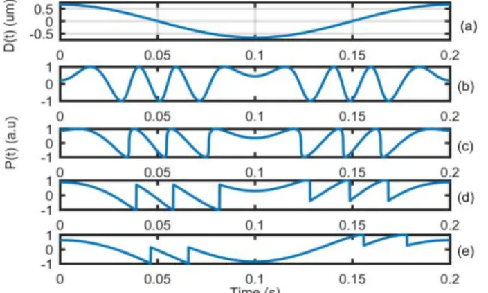
Fig. 2. Simulated SM Signals for different C values with target vibration 𝐴𝑝−𝑝
= 1.7 λ0 (λ0 = 785nm) (a) D(t), (b) C = 0.2, (c) C = 1, (d) C = 2.5, (e) C = 5.
In another SMI setup, for a determined amount of optical feedback, an internal sub-periodicity appeared in SMI signals due to mode hopping between the different longitudinal laser modes excited by the external cavity [23]. SMI sensor resolution could then be doubled or tripled due to multiple modes undergoing SMI [23].
Similarly, in the context of avoiding any external optical component, Zheng et al. proposed a simple and fast even-power scalable algorithm (EPSA) for improving fringe resolution in SMI [1]. This method is based on a signal processing technique, in which a weak optical feedback regime [1, 2] SMI signal is passed through multiple stages. At each stage, square of signal is subtracted from scaled version of original signal resulting in doubling of fringe resolution after each stage. Results showed that EPSA [1] provided up to λ0/32 fringe resolution for SMI
signals as long as optical feedback coupling factor C remained stable and very small, corresponding to so-called weak feedback regime (C <1) [1].
EPSA thus provided an elegant signal processing based method for improving the SMI resolution. However, certain limitations remain before it can be used for practical, real-world sensing applications in which optical feedback strength cannot be kept constant at all times. Practically, variations in optical feedback do occur during the course of continuous sensing (resulting in change from weak- to moderate- or strong-optical feedback regime or vice-versa). Furthermore, speckle phenomenon [24], causing fringe amplitude variation [25] and regime-change [26], can also occur in case of non-cooperative remote target surfaces. As the shape and amplitude of SMI signal is strongly dependent on 1) optical feedback strength and 2) speckle, so performance of EPSA significantly degrades due to variation in these two factors.
In addition to above-mentioned two limitations, EPSA [1] employed sampling frequency 𝑓𝑠 of 50 kHz even when remote
target’s velocity was low (maximum measurable target’s velocity is proportional to 𝑓𝑠), and could not process SM signals
acquired using lower 𝑓𝑠. Even when such a high 𝑓𝑠 (with respect
to actual target’s velocity) was chosen, the measurement resolution remained limited to λ0/32 (due to inherent bandwidth
Lastly, EPSA was discussed only in the context of off-line sensing/processing [1]. Thus, no hardware-implementation architecture was proposed to ascertain the performance of EPSA for later practical, real-time, embedded implementation. In this context, the aim of this work is to present solutions to each of above-mentioned 4 limitations of EPSA [1]. The proposed algorithm allows the use of EPSA even when large variation in optical feedback occurs such that SMI sensor enters the so-called moderate-, or even strong- optical feedback regime. Furthermore, it is also able to process such SMI signals exhibiting signal fading due to occurrence of speckle. Also, EPSA is modified to enable processing of SMI signals at lower sampling rates. Lastly, field programmable gate array (FPGA) based hardware emulation of EPSA is also performed for potential implementation enabling embedded sensing.
II. THEORY OF SMI
Theory of SMI is well-established [2, 3], and is summarized below. SMI occurs when emitted laser strikes a remote target under displacement 𝐷(𝑡) and a part of the backscattered light re-enters the active laser cavity. There, it interacts with emitting field causing change in optical output power (OOP) signal P(t) received at photo-diode (PD), given by :
𝑃(𝑡) = 𝑃0[1 + 𝑚 ∗ Cos(Φ𝐹(𝑡)] (1)
where m is modulation index, ΦF(t) is laser output phase with
optical feedback and P0 is OOP of free running laser emitting
wavelength λ0 [2].
In SMI, C is a fundamental parameter categorizes an SM signal into three main categories:
1) 0.1 < C < 1 characterizes weak optical feedback regime with SMI signal having sinusoidal or quasi-sinusoidal fringes without sharp discontinuities.
2) 1 < C < 4.6 characterizes moderate feedback regime with fringes having saw-tooth like shape and asymmetric hysteresis. 3) C > 4.6 results in strong feedback regime signal with chaotic shape and fringe-loss.
Note that when C increases, hysteresis in SMI signal increases, height of SMI fringes decreases, and fringes begin to disappear for strong feedback regime (see Fig. 2).
III. EPSALIMITATIONS AND PROPOSED SOLUTIONS EPSA is based on the approximation that for weak regime, feedback phase ΦF(t) does not change greatly and can be
approximated as Φ0(t). Then P(t) can be modulated directly by
cosine of the phase as any traditional interferometric system.
𝑃(𝑡) = 𝑐𝑜𝑠[Φ0(𝑡)] (2)
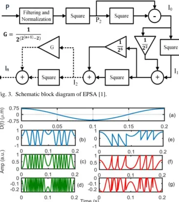
So, by raising the power to double, triple and quadruple, resolution doubles, triples and quadruples accordingly. Fig. 3 shows schematic block diagram of EPSA, where P2, I0, I1, I2
and In represents 1st, 2nd, 3rd, 4th and nth stage output
respectively. After each stage, fringe resolution was doubled, theoretically leading to 𝑛𝑡ℎ stage for which fringe resolution
can be given by 𝜆0⁄ 2𝑛+3. In the case of moderate and strong
regime, above EPSA approximation does not hold, resulting in inability to process moderate and strong regime signals. That is
redistribution to servers or lists, or reuse of any copyrighted components of this work in other works. why; the suggested approach is to replace the discontinuous
fringes by continuous one that looks like the weak feedback regime.
Fig. 3. Schematic block diagram of EPSA [1].
Fig. 4. Performance of EPSA for high- and low-C valued simulated SMI signals with 𝐴𝑝−𝑝 = 1.7 λ0 (λ0 = 785 nm) (a) D(t), (b) - (d) normalized P(t) for C=0.2,
1st stage output (P
2) and 2nd stage output (I0) for signal (b), (e) - (f) normalized
P(t) for C=3, 1st stage- (P
2) and 2nd stage-output (I0) for signal (e).
As previously mentioned, EPSA had following limitations, which need to be addressed:
1) EPSA cannot process SMI signals belonging to moderate-
and strong-optical feedback regime.
2) EPSA cannot process speckle affected SMI signals
exhibiting signal fading, and requires stable optical feedback.
3) EPSA does not address the aspect of bandwidth expansion
of SMI signal leading to limitation in resolution improvement.
4) EPSA is validated for off-line SMI signals only. I.e., no
hardware implementation/architecture is proposed for real-time, embedded sensing applications.
This section is further divided into 5 subsections addressing each of the above-mentioned limitations of EPSA culminating in the proposed improved EPSA, denoted as IEPSA.
A. Large Variation in Optical Feedback Strength
As previously discussed, EPSA [1] can only process weak-feedback regime signals (C<1), and cannot process high C value signals of moderate- and strong-feedback regimes.
Fig. 4 shows comparison of EPSA processing results for weak- and moderate-feedback regime SMI signal with C=0.2 and C=3 respectively for a target vibration of Ap-p = 1.7 λ0. It is
clearly seen that EPSA is able to process weak-feedback regime signal (see Fig. 4(b)-4(d)), but is unable to process moderate-feedback regime signal (see Fig. 4 (e-g)).
With the increase in C, the shape of SMI fringes changes from sinusoidal to saw-tooth like, and fringe-amplitude also
decreases (see Fig. (2)). The objective then is to reshape an SMI signal with high C value into an SMI signal pertaining to low C value resulting in a signal procesable through EPSA.
Fig. 5. Schematic block diagram of signal reshaping method enabling the processing of moderate- and strong-feedback regime SM signals.
Fig. 6. Signal reshaping method on simulated SM signal with C=1.8 for target vibration with 𝐴𝑝−𝑝 = 1 λ0 (λ0 = 785nm): (a) D(t), (b) normalized P(t) (blue),
and fringes (red) (c) reshaped signal.
The proposed SM signal reshaping method is schematically presented in Fig. 5 while Fig. 6 shows the results of signal reshaping applied on an SMI signal with C=1.8.
In Fig. 5, 𝑃[𝑛] denotes the digitized version of P(t). First, amplitude of signal is normalized within 1 and -1, then
normalized signal is passed through fringe
detection/localization block, which is based on derivative followed by thresh-holding for fringe detection. Then, localization for finding exact fringe location is performed by searching for max-min location around the detected fringe. Fringe location and fringe direction information is used in signal segmentation block to segment it into hump region and fringe region. After segmentation of signal, fringe regions are processed differently, while hump region is processed differently using reshaping techniques, as explained ahead.
It is known from [27], that the phase travel from the start of one fringe to the start of other fringe is 2π in the absence of fringe loss. Therefore, to reshape the fringe regions, a cosine wave generator is used to replace the signal between any two consecutive fringes with a cosine waveform starting from one fringe location and ending at other the other consecutive fringe while traveling 2π phase (see vertical green lines Fig. 6 (b-c)). Hump region is the region between two opposite direction fringes. Hump region is further sub-divided into two parts, i.e. upward going hump and downward going hump. Purple vertical lines between two green lines in Fig. 6(b-c) indicate the distribution of hump regions in to two parts. Left part of the
and ending before the start of next part (purple line fig. (6c)). Similarly, other half of hump is also replaced with cosine wave ending at the next fringe location (as indicated in Fig (6c)). Fig. 6 shows the successful processing of C=1.8 and 𝐴𝑝−𝑝= 1λ0
signal using proposed reshaping method.
B. Speckle Affected SMI Signals
After employing signal reshaping, SM signals with any C value (belonging to weak-, moderate- or strong-feedback regime (inclusive of fringe-loss [6] at the cost of lower resolution)) can now be processed. However, efforts need to be undertaken so that SMI signals with speckle can also be processed by the proposed method.
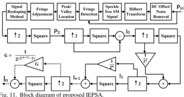
Speckle phenomenon happens due to constructive and destructive superposition between multiple light beams reflected from a rough target surface [24]. This causes rapid fringe amplitude fading at different points in received SM signal as highlighted in Fig. 7(a) [26]. As a result, again EPSA cannot correctly process such a signal due to sharp amplitude variations. In this regard, Hilbert Transform (HT) based SMI signal processing [28] has been proposed for speckle affected signals. So, HT is now used in conjunction with the method of
Section III-A to deal with speckle affected SMI signals. Block
diagram of HT based processing is shown in Fig. 8. Firstly, any DC offset of speckle affected SMI signal is removed by using a 64-tap moving average filter.
Secondly, HT is applied resulting in retrieval of an instantaneous phase (IP) signal which is devoid of amplitude variations caused by speckle (see Fig. 7(b)-(c)) [28].
This IP signal, however, contains fast switching at fringe locations (see Fig. 7 (c)) which necessitates reshaping of this IP signal. So, it is processed using the previously described signal reshaping method to obtain equivalent signal with cosine fringes (see Fig. 7 (d)).
Fig. 7. Signal processing of speckle affected SM Signal: (a) normalized P(t), (b) instantaneous phase (IP) retrieval after Hilbert transform, (c) zoomed version of signal shown in (b), and (d) signal reshaping method applied on (c).
Fig. 8. Signal reshaping of speckle-affected SMI signal using Hilbert transform (HT) based method.
Fig. 9. Block diagram of IEPSA for processing SMI signal at optimum sampling frequency. 1st stage, 2nd stage and nth stage represents 1st, 2nd and nth
output stage of EPSA respectively.
Fig. 10. Performance comparison of EPSA in case of low-rate sampled SM Signal with C=0.2 and 𝐴𝑝−𝑝 = 1 λ0 (λ0 = 785nm), sampled at fopt = 1.25 kHz (a)
𝐷(𝑡), (b) normalized P(t), (c) EPSA P2 stage output and (d) EPSA 3rd stage
output (e) zoomed version of EPSA 3rd stage output, (f) normalized 𝑃(𝑡), (g)
Interpolated EPSA P2 stage output, (h) interpolated EPSA 3rd stage output, and
(i) zoomed version of interpolated EPSA 3rd stage output.
Fig. 11. Block diagram of proposed IEPSA.
C. Bandwidth Expansion and Optimal Sampling Rate
As already mentioned, EPSA did not address SMI signal’s bandwidth expansion (at each multiplicative stage) and employed a high 𝑓𝑠 to mitigate its effect on limitation of
resolution improvement. Specifically, it [1] could only process SMI signals sampled at ≥ 50 kHz.
However, 𝑓𝑠 needs to be set according to the maximum target
velocity𝑣𝑚𝑎𝑥 and thus depends on maximum peak to peak
amplitude 𝐴𝑝−𝑝𝑚𝑎𝑥 and frequency 𝑓𝑡𝑚𝑎𝑥 of target motion
𝐷(𝑡) =𝐴𝑝−𝑝𝑚𝑎𝑥
2 sin(2𝜋𝑓𝑡𝑚𝑎𝑥𝑡). Thus,
𝑣𝑚𝑎𝑥 = 𝜋𝑓𝑡𝑚𝑎𝑥𝐴𝑝−𝑝𝑚𝑎𝑥 (3)
At the fringe level (Δ𝐷 = 𝜆0/2), minimum duration of fringe
Δt becomes:
Δ𝑡 = Δ𝐷
𝑣𝑚𝑎𝑥=
𝜆0
2𝜋𝑓𝑡𝑚𝑎𝑥𝐴𝑝−𝑝𝑚𝑎𝑥 (4)
If one sample per fringe is taken using𝑓𝑢𝑛𝑖𝑡 = 1/Δ𝑡, then
𝑓𝑢𝑛𝑖𝑡=
2𝜋𝑓𝑡𝑚𝑎𝑥𝐴𝑝−𝑝𝑚𝑎𝑥
𝜆0 (5)
Note that if 𝑓𝑠= 𝑓𝑢𝑛𝑖𝑡, sampled displacement resolution (in
terms of 𝐷[𝑛]– 𝐷[𝑛 − 1]) is only of 𝜆0
2. Nevertheless, such a
redistribution to servers or lists, or reuse of any copyrighted components of this work in other works. be at least twice of this frequency to fulfill Shannon principle.
Thus, to increase sampled displacement resolution, higher number of samples per fringe 𝑁𝑓𝑟is required. (Higher 𝑁𝑓𝑟
enables better resolution of peak- and valley-instants as well.) Thus, optimum sampling frequency fopt becomes:
𝑓𝑜𝑝𝑡 = 𝑁𝑓𝑟
2𝜋𝑓𝑡𝑚𝑎𝑥𝐴𝑝−𝑝𝑚𝑎𝑥
𝜆0 (6)
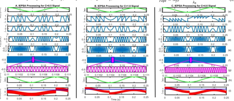
Fig. 12. IEPSA response for simulated SM signals for (A) weak feedback regime (C=0.5), (B) moderate feedback regime (C=1.8) and (C) strong feedback regime (C=4.6), (a) target displacement 𝐷(𝑡) (b) P (t), (c) fringe reshaping, (d) P2, (e) I0, (f) I9, (g) zoomed view of I9, (h) retrieved target displacementby fringe counting
and (i) peak-peak error (red line) and RMS error (blue line) between reference displacement and retrieved displacement.
Fig. 13. Block diagram of FPGA based hardware emulation of IEPS. Note that peak/valley locations are required for fringe adjustment (see Fig. 5), and are also used for accurate phase unwrapping in advanced SMI algorithms [27, 29]. Simulations indicate that if 𝑁𝑓𝑟≥ 40 then it is possible to accurately
localize peak- and valley-instants. Likewise, 𝑁𝑓𝑟≥ 40 can
theoretically ensure sample displacement resolution of ≥ 𝜆0
80.
After specifying 𝑓𝑜𝑝𝑡, let us discuss how the performance of
EPSA is affected by 𝑓𝑠. In EPSA, number of fringes in input
SMI signal are doubled after every stage due to multiplication of signal with itself, as given by [1]:
𝐼𝑛= (𝐼𝑛−1∗ 𝐼𝑛−1) + 1
2(2𝑛+1)𝐼𝑛−1 (7)
Where In and In-1 are the 𝑛𝑡ℎ and (𝑛 − 1)𝑡ℎstage outputs.
Signal multiplication with itself results in doubling of signal bandwidth (BW), as evident by the identity:
cos(𝜔0𝑡) ∗ cos(𝜔0𝑡) = 0.5 ∗ [1 + cos(2𝜔0𝑡)] (8)
Consequently, the BW of the input SMI signal doubles after every stage. EPSA catered to high BW of later stages by introducing a very high fs at the input ADC stage (where P(t) is
originally discretized). Thus, this very high fs was set well
beyond the optimum fs. Consequently, very high fs enabled to
cater to BW expansion up till 4 stages but it is not the right solution to the problem of BW expansion.
On the other hand, in the proposed work, fs of ADC is
adjusted to the optimum fs (which can now be set in proportion
to maximum measurable target velocity) while BW expansion (by factor of 2) of the signal within each stage is dealt with by using dyadic up-sampling and interpolation.
Fig. 9 presents the block diagram of our proposed solution of BW expansion problem while processing SMI signal at fopt.
1𝑠𝑡, 2𝑛𝑑,and𝑛𝑡ℎ stage block denote 1𝑠𝑡, 2𝑛𝑑,and𝑛𝑡ℎ output
stage of EPSA respectively. Fig. 10 shows the comparison of performance of EPSA with (Fig. 10 (f)-(i)) and without (Fig. 10(b)-(e)) interpolation for an SMI signal having C=0.2, f0=5
Hz and Ap-p = λ0 sampled at𝑓𝑜𝑝𝑡 of 1.25 kHz, as per (8). Without
dyadic up-sampling and interpolation, SMI signal shape is significantly distorted even after the 2nd stage of EPSA.
D. Improved EPSA (IEPSA) and Simulated Results
Finally, after these three improvements presented in III-A,
III-B and III-C, a new improved version of EPSA (denoted
IEPSA) is proposed (see complete block diagram in Fig. 11). IEPSA is tested on simulated SMI signals pertaining to different feedback regimes. Fig. 12 shows successful IEPSA processing of simulated SMI signals of three different optical feedback regimes, i.e. weak-, moderate- and strong-feedback regime, with 𝐶 value of 0.5, 1.8,and4.6 respectively.
All SMI signals are processed up to 10 stages. 10𝑡ℎ stage
output is also used to reconstruct the target motion by fringe-counting (or accumulation of all duplicated fringes). Note that this process introduces small errors in the reconstruction of the displacement thereby decreasing the precision of retrieved motion. Comparison with reference target motion is also done resulting in RMS error or displacement reconstruction precision of 0.4𝑛𝑚 (≅ 𝜆0 211), 0.8𝑛𝑚 (≅ 𝜆0 210)and0.9𝑛𝑚 (≅ 𝜆0 210) for
respectively. As the theoretical resolution for 𝑛 stage EPSA output is given by λ0
2𝑛+3 [1] so, for 10
𝑡ℎstage output, it is compares favorably with the theoretical resolution.
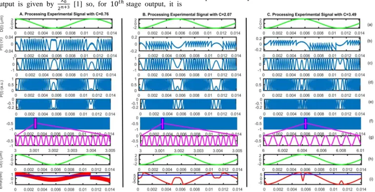
Fig.14 IEPSA results for experimental SMI signals for (A) C=0.76, (B) C=2.07 and (C) C=3.49, (a) acquired target displacement 𝐷(𝑡) from reference PZT sensor (b) P(t), (c) fringe reshaping, (d) P2, (e) I0, (f) I9, (g) zoomed view of I9, (h) retrieved Displacement by fringe counting and (i) peak-peak error (red line) and RMS
error (blue line) between PZT displacement and retrieved displacement TABLE I. RESOURCES CONSUMPTION DETAILS FOR EPSA ON VIRTEX-6
Resources Utilization % Utilization
Slice Registers 15,454 20 %
LUTs 13042 8.8 %
Slices 4,130 35 %
LUT Flip Flop pairs 13203 14 %
TABLE II. POWER CONSUMPTION DETAILS FOR EPSA ON VERTEX-6
On-Chip Power Consumption
(mW) Total Dynamic power 622
Quiescent Power 780
Total power (Dynamic + quiescent) 1402
However, with the increase in 𝐶, precision values decreases. This can be understood by realizing that when increasingly saw-tooth shaped fringes (for higher 𝐶) are replaced by cosine-shaped fringes, then more and more information from SMI signal’s original phase is lost in this transformation. Another source of imprecision is the uncertainty in exact fringe location detection. Furthermore, in case of fringe-loss, precision expectedly further decreases for strong feedback regime [7].
E. Hardware Emulation
FPGA based hardware emulation of IEPSA is done using Vertex-6 XC6VLX75T as target device. VHSIC (Very High Speed Integrated Circuit) Hardware Description Language (VHDL) is used for this purpose using Xilinx ISE tool. 32-bit fixed-point precision is used for IEPSA emulation by taking 16-k samples of normalized SMI signal in Q1.31 format.
Currently, IEPSA design is emulated on FPGA up to five output stages (design can easily be scaled to 𝑛 output stages). In addition to EPSA [1], HT based speckle affected SMI signal processing is also implemented. The hardware design can thus be divided into four sub-blocks i.e. DC removal, Hilbert transform, IP retrieval, and five-stage EPSA (Fig. 13).
DC removal block (consisting of moving average filter of 64 taps) is designed using VHDL language in Xilinx ISE tool.For Hilbert transform block implementation, 16-k points FFT/IFFT cores available in Xilinx ISE tool are used.
Similarly, for IP block, Cordic core is used to find arctan followed by arctan to arctan2 block in order to recover Hilbert phase signal for complete 3600 plane.
The FPGA based IEPSA system can operate at maximum clock frequency of 255 MHz with latency of 261k clock cycles. Table I presents the resource utilization and Table II presents power consumption detail of our design.
As per (6), maximum measurable velocity is given by: 𝑣𝑚𝑎𝑥 = 𝑓𝑜𝑝𝑡
𝜆0
2𝑁𝑓𝑟 (9)
For a laser with 𝜆0= 785𝑛𝑚, an ADC operating at 120
MHz, and 𝑁𝑓𝑟≥ 40, 𝑣𝑚𝑎𝑥= 1.18𝑚/𝑠. This means that our
system could be used for sensing applications with high bandwidth requirement such as measurement of ultrasonic vibrations. For example, for target vibration occurring at 50 kHz, proposed FPGA based emulation of IEPSA can recover such vibration having 𝐴𝑝−𝑝 up to 7.5𝜇𝑚.
redistribution to servers or lists, or reuse of any copyrighted components of this work in other works. IV. EXPERIMENTAL RESULTS
The proposed IEPSA is tested by using a variety of experimental SMI signals under different optical feedback regime-, speckle-, and target motion-conditions. A commercial PZT (Piezo-electric Transducer) from Physik Instrumente® is
used as the remote target. The PZT is equipped with a built-in capacitive sensor of 2𝑛𝑚 measurement precision, used as a reference to quantify the measurement performance of IEPSA.
Fig. 15. IEPSA response for an experimental speckle affected SM signal. (a) normalized 𝑃(𝑡), (b) phase retrieval after Hilbert transform (HT), (c) zoomed version of signal (b), (d) signal reshaping applied on (c), (e) P2, (f) I0, (g) I9, and
(h) zoomed view of I9.
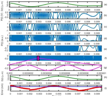
Fig. 16. IEPSA performance for an experimental SMI signal corresponding to arbitrary target motion. (a) reference displacement from PZT (b) P(t), (c) fringe reshaping, (d) P2, (e) I0, (f) I9, (g) zoomed view of I9, (h) retrieved displacement,
and (i) error (red line) and RMS error (blue line).
The SMI sensor is based on LD package from Sanyo®
(DL7140) with 𝜆0= 785𝑛𝑚, emitting power of 60𝑚𝑊, and
a threshold current of 50𝑚𝐴. The built-in monitor photo-diode of DL7140 was used to acquire the SMI signals. Sand paper was pasted on the normally polished metallic surface of PZT to acquire speckle affected signal. Optical feedback strength was varied by changing the focus of the lens (having 6.24𝑚𝑚 focal length) mounted inside the collimation tube (model LT110P-B by ThorLabs®) which housed the LD.
IEPSA is tested on experimental SMI signals pertaining to weak-, moderate- and strong-optical feedback regime. 10th
stage output of IEPSA is also used to reconstruct the target motion. Comparison with reference PZT sensor’s motion is also carried out to obtain measurement accuracy results. Fig. 14 presents successful processing of experimental SMI signals with estimated values of 𝐶 = 0.76, 𝐶 = 2.07and𝐶 = 3.49 having precision of 0.8𝑛𝑚 (≅ 𝜆0
210) , 4.8𝑛𝑚 (≅
𝜆0
28)and5𝑛𝑚
(≅𝜆0
27) respectively. (Note that phase unwrapping based method
[28] was used to estimate 𝐶 values.). More simulation are conducted for C>4.6, and precision of 35 nm, 54 nm and 70 nm was observed for C= 5.13, 6.8 and 7.3 respectively, with fringe loss of 1, 2 and 2. Low IEPSA precision for strong feedback-regime expectedly occurred due to disappearance of one SMI fringe [7]). Importantly, IEPSA performance for experimental weak-, and moderate-feedback SMI signals approaches that of PZT sensor which itself has a precision of 2𝑛𝑚 (≅ 𝜆0
29).
IEPSA is capable of processing speckle-affected experimental SM signals as well (see Fig. 15). Similarly, IEPSA is also able to process SMI signals corresponding to arbitrary motion of PZT target. Fig. 16 shows successful processing of such an SMI signal using IEPSA, resulting in RMS error of 5 nm (≅𝜆0
28).
V. CONCLUSION
In SMI, many algorithms have been proposed to improve basic fringe resolution beyond λ0/2. One of those algorithms is
EPSA [1]. In this work, EPSA is analyzed, its limitations are found and a new improved version of EPSA (IEPSA) overcoming all the identified limitations of previous work is proposed. It is now able to process SMI signals belonging to all major optical feedback regimes encountered in SMI as well as speckle affected signals. The upper limit of scaling for practical sensing is also now removed. Testing and verification of our system is done with both simulated- and variety of experimental-SMI signals. Furthermore, FPGA based hardware emulation of IEPSA is also done, indicating that our designed system can operate at a clock frequency of 255 MHz while consuming total power of 1.4 W with maximum measurable velocity of1.18𝑚/𝑠. The successful implementation of this high resolution method leads towards a complete autonomous SMI setup for real-world sensing.
REFERENCES
[1] Z. Wei, W. Huang, J. Zhang, X. Wang, H. Zhu, T. An, et al., "Obtaining Scalable Fringe Precision in Self-Mixing Interference Using an Even-Power Fast Algorithm," IEEE Photonics Journal, vol. 9, pp. 1-11, 2017.
[2] T. Taimre, M. Nikolić, K. Bertling, Y. L. Lim, T. Bosch, and A. D. Rakić, "Laser feedback interferometry: A tutorial on the self-mixing
[3] S. Donati, "Developing self‐mixing interferometry for instrumentation and measurements," Laser & Photonics Reviews, vol. 6, pp. 393-417, 2012.
[4] Y. Zhao, S. Wu, R. Xiang, Z. Cao, Y. Liu, H. Gui, et al., "Self-mixing fiber ring laser velocimeter with orthogonal-beam incident system," IEEE Photonics Journal, vol. 6, pp. 1-11, 2014. [5] A. Ehtesham, U. Zabit, O. Bernal, G. Raja, and T. Bosch, "Analysis
and Implementation of a Direct Phase Unwrapping Method for Displacement Measurement using Self-Mixing Interferometry,"
IEEE Sensors Journal, vol. 17, pp. 7425-7432, 2017.
[6] S. Donati, D. Rossi, and M. Norgia, "Single Channel Self-Mixing Interferometer Measures Simultaneously Displacement and Tilt and Yaw Angles of a Reflective Target," IEEE Journal of Quantum
Electronics, vol. 51, pp. 1-8, 2015.
[7] M. Veng, J. Perchoux, and F. Bony, "Fringe Disappearance in Self-Mixing Interferometry Laser Sensors: Model and Application to the Absolute Distance Measurement Scheme," IEEE Sensors Journal, 2019.
[8] Z. A. Khan, U. Zabit, O. D. Bernal, M. O. Ullah, and T. Bosch, "Adaptive Cancellation of Parasitic Vibrations Affecting a Self-Mixing Interferometric Laser Sensor," IEEE Transactions on
Instrumentation and Measurement, vol. 66, pp. 332-339, 2017.
[9] M. Norgia, A. Pesatori, and L. Rovati, "Self-mixing laser Doppler spectra of extracorporeal blood flow: a theoretical and experimental study," IEEE Sensors Journal, vol. 12, pp. 552-557, 2012. [10] Y. Tan, W. Wang, C. Xu, and S. Zhang, "Laser confocal feedback
tomography and nano-step height measurement," Scientific reports, vol. 3, p. 2971, 2013.
[11] P. Dean, A. Valavanis, J. Keeley, K. Bertling, Y. Leng Lim, R. Alhathlool, et al., "Coherent three-dimensional terahertz imaging through self-mixing in a quantum cascade laser," Applied Physics
Letters, vol. 103, p. 181112, 2013.
[12] C. Chen, Y. Zhang, X. Wang, X. Wang, and W. Huang, "Refractive index measurement with high precision by a laser diode self-mixing interferometer," IEEE Photonics Journal, vol. 7, pp. 1-6, 2015. [13] T. Hou, C. Zheng, S. Bai, Q. Ma, D. Bridges, A. Hu, et al.,
"Fabrication, characterization, and applications of microlenses,"
Applied optics, vol. 54, pp. 7366-7376, 2015.
[14] J. Wu, G. Ding, X. Chen, T. Han, X. Cai, L. Lei, et al., "Nano step height measurement using an optical method," Sensors and
Actuators A: Physical, vol. 257, pp. 92-97, 2017.
[15] C. Nwafor, W. Mo, D. King, A. Shringarpure, and K. Plant, "Importance of Illumination in a Non-Contact Photoplethysmography Imaging System for Burn Wound Assessment," Int J Opt Photonic Eng, vol. 4, p. 016, 2019. [16] X. Cheng and S. Zhang, "Intensity modulation of VCSELs under
feedback with two reflectors and self-mixing interferometer,"
Optics communications, vol. 272, pp. 420-424, 2007.
[17] L. Wang, X. Luo, X. Wang, and W. Huang, "Obtaining high fringe precision in self-mixing interference using a simple external reflecting mirror," IEEE Photonics Journal, vol. 5, pp. 6500207-6500207, 2013.
[18] Z. Zeng, X. Qu, Y. Tan, R. Tan, and S. Zhang, "High-accuracy self-mixing interferometer based on single high-order orthogonally polarized feedback effects," Optics express, vol. 23, pp. 16977-16983, 2015.
[19] D. Melchionni, A. Magnani, A. Pesatori, and M. Norgia, "Development of a design tool for closed-loop digital vibrometer,"
Applied optics, vol. 54, pp. 9637-9643, 2015.
[20] G. Giuliani, S. Bozzi-Pietra, and S. Donati, "Self-mixing laser diode vibrometer," Measurement Science and Technology, vol. 14, p. 24, 2002.
[21] Z. Huang, C. Li, S. Li, and D. Li, "Equivalent wavelength self-mixing interferometry for displacement measurement," Applied
optics, vol. 55, pp. 7120-7125, 2016.
[22] C. Jiang, Z. Zhang, and C. Li, "Vibration measurement based on multiple self-mixing interferometry," Optics Communications, vol. 367, pp. 227-233, 2016.
[23] M. Ruiz-Llata and H. Lamela, "Self-mixing technique for vibration measurements in a laser diode with multiple modes created by optical feedback," Applied optics, vol. 48, pp. 2915-2923, 2009.
vol. 49, pp. 798-806, 2013.
[25] O. Bernal, H. C. Seat, U. Zabit, F. Surre, and T. Bosch, "Robust Detection of Non Regular Interferometric Fringes from a Self-Mixing Displacement Sensor using Bi-Wavelet Transform," IEEE
Sensors Journal, vol. 16, p. 7903, 2016.
[26] A. A. Siddiqui, U. Zabit, O. D. Bernal, G. Raja, and T. Bosch, "All Analog Processing of Speckle Affected Self-Mixing Interferometric Signals," IEEE Sensors Journal, vol. 17, pp. 5892-5899, 2017. [27] O. D. Bernal, U. Zabit, and T. Bosch, "Study of laser feedback phase
under self-mixing leading to improved phase unwrapping for vibration sensing," IEEE Sensors Journal, vol. 13, pp. 4962-4971, 2013.
[28] A. L. Arriaga, F. Bony, and T. Bosch, "Real-time algorithm for versatile displacement sensors based on self-mixing interferometry," IEEE Sensors Journal, vol. 16, pp. 195-202, 2016. [29] Y. Fan, Y. Yu, J. Xi, and J. F. Chicharo, "Improving the measurement performance for a self-mixing interferometry-based displacement sensing system," Applied Optics, vol. 50, pp. 5064-5072, 2011.
Saqib Amin received the M.S. degree in electrical engineering from Riphah International University, Islamabad, Pakistan, in 2016. He is currently a Lecturer at Riphah International University.His research interests include digital design and signal processing for sensingapplications.
Usman Zabit (M’12–SM’19) received the Ph.D. degree from the Institut National Polytechnique Toulouse (INPT), France, in 2010. He is currently an Associate Professor with the National University of Sciences and Technology, Islamabad, Pakistan. Dr Zabit was a recipient of the Prix Leopold Escande 2010 and the European Mechatronics Award from INPT and the European Mechatronics Meeting 2010, respectively.
Olivier D. Bernal (M’03) received the M.Sc. degree in electrical engineering and the Ph.D. degree from the Institut National Polytechnique Toulouse(INPT), Toulouse, France, in 2003 and 2006, respectively. He joined the Laboratory of Optoelectonics and Embedded Systems,LAAS-CNRS, and INPT in 2009, where he is currently an Assistant Professor. His main research interests are in analog circuit design for optoelectronics andspace applications.
Tassadaq Hussain received Ph.D. degree in computer architectures at the Universitat Politécnica de Catalunya (UPC), Spain. He obtained MSc (Electronics) degree in 2009 from the Institut Supérieur d’Electronique de Paris France. He is currently Associate Professor at Riphah International University, Pakistan. His research interests include digital design and supercomputing for artificial Intelligence applications.