HAL Id: inria-00422970
https://hal.inria.fr/inria-00422970
Submitted on 8 Oct 2009
HAL is a multi-disciplinary open access
archive for the deposit and dissemination of
sci-entific research documents, whether they are
pub-lished or not. The documents may come from
L’archive ouverte pluridisciplinaire HAL, est
destinée au dépôt et à la diffusion de documents
scientifiques de niveau recherche, publiés ou non,
émanant des établissements d’enseignement et de
Dynamic Compartments in the Imperative Pi Calculus
Mathias John, Cédric Lhoussaine, Joachim Niehren
To cite this version:
Mathias John, Cédric Lhoussaine, Joachim Niehren. Dynamic Compartments in the Imperative Pi
Cal-culus. Computational Methods in Systems Biology, 7th International Conference, Aug 2009, Bologna,
Italy. pp.235-250, �10.1007/978-3-642-03845-7�. �inria-00422970�
Dynamic Compartments in the
Imperative π-Calculus
Mathias John1, C´edric Lhoussaine24, and
Joachim Niehren34
1 University of Rostock, Computer Science, Modeling and Simulation Group 2 University of Lille 1
3 INRIA, Lille, Mostrare
4 BioComputing, LIFL (CNRS UMR8022) & IRI (CNRS USR3078)
Abstract. Dynamic compartments with mutable configurations and variable volumes are of basic interest for the stochastic modeling of biochemistry in cells. We propose a new language to express dynamic compartments that we call the imperative π-calculus. It is obtained from the attributed π-calculus by adding imperative assignment operations to a global store. Previous approaches to dynamic compartments are im-proved in flexibility or efficiency. This is illustrated by an appropriate model of osmosis and a correct encoding of BioAmbients.
1
Introduction
Concurrent control is crucial for the stochastic modeling of biochemical processes in living cells [19, 2, 13]. The regulation of such systems depends on all kinds of physical or chemical aspects, such as volume, surface, temperature, pressure, pH value, spatial coordinates and structures. Most of these aspects are of global nature, so they require modeling languages in which global concurrent control can be expressed [20]. In this paper, we present a new modeling language, that permits to express many aspects with global control in a uniform manner, and illustrate its usefulness by modeling dynamic compartments with mutable vol-umes and surfaces.
Dynamic compartments may change their nesting structure dynamically, by applying operations for compartment creation, removal and merging. These op-erations may influence the speed of diverse reactions within compartments, in particular when compartment volumes change (global to local interactions). Vice versa, local reactions within a single compartment may effect global numeric attributes such as volume and surface (local to global interaction). Various lan-guages for modeling systems with dynamic compartments were proposed for sys-tems biology [18, 14, 21], but none of them can express physical, chemical, and compartimental aspects in a uniform manner, while providing efficient stochastic simulation. Spatial languages such as the Brane Calculi [2] or BioAmbients [18] fix a particular set of operators on compartments, and provide a special pur-pose solution for these operations. The π-calculus with polyadic synchronization
inria-00422970, version 1 - 8 Oct 2009
and global priorities π@ is more flexible, in that it permits to encode all kinds of compartment structures, including those of Brane Calculi and BioAmbients [20]. Unfortunately, such priority-based encodings are complex, low level, and in-efficient. Consider e.g. the dissolving of a compartment with n equal molecules. Informing all of them requires O(n) interactions rather than O(1) by updating all at once. Furthermore, π@ lacks general support for stochastic rates and numeric attributes such as volumes and pH-values. The only solution to compartments with variable volumes so far [21] was expressed in the special purpose dialect called Sπ@. Numerical attributes of compartments are equally lacking in
Bi-graphs [14, 12], a modeling language for spatial dynamics based on a particular
form of hypergraph rewriting. Thus, the question is whether there exists a better general purpose language for expressing dynamic compartments.
In this paper, we start from the attributed π-calculus [11], and enrich it by an imperative store for global control. The attributed π-calculus is parametrized by a sequential higher-order language L for describing all kinds of values (symbolic and numeric) and constraints. It features “attributed” processes A(e1, . . . , en)
with values defined by expressions e1, . . . , en of L. For instance, cells with
vari-able volumes vol can be modeled by using a single attribute:
Cell(vol)! enter[λr. if r<0.1 then (val enter)]?(v).Cell(vol + v)
The input prefix contains a function in square brackets, that tests for ev-ery matching output prefix, whether the reaction is permitted and returns its stochastic rate in this case. Cells as above can be entered by elements Ele(r, v) of radius r and volume v, if r is smaller than 0.1:
Ele(r, v)! enter[r]!(v).0
Under this condition, the stochastic rate of the enter reaction is obtained by evaluating the expression (val enter), i.e., by accessing the value of channel enter from the environment. As a result of the reaction, the cell volume is increased by v. The entered elements disappear, since we chose to not represent elements in cells explicitly here.
We obtain the imperative π-calculus πimp(L), by allowing imperative
pro-gramming languages L as attribute language. Thereby, we enrich the π-calculus by a global imperative store. More precisely, we add assignment expressions to
L by which to change the values of channels dynamically, such as for instance enter := val enter + 1.5, whose evaluation increases the value of channel enter
by 1.5. The expressions of L are evaluated as transactions, so that the evaluator cannot be interrupted by any other process. We present a stochastic semantics for πimp(L) that properly accounts for transactions with imperative assignments.
We show how to compile processes of πimp(L) to stochastic simulators,
indepen-dently of the choice of parameter L. We have implemented the compiler and can report on first experimental results. To this purpose, we model a simple exam-ple of osmosis in πimp(L) where variable volumes and surfaces matter. Practical
simulation experiments confirm higher accuracy compared to [21] due to variable surfaces (not only volumes) and good efficiency.
In order to provide a more systematic treatment of dynamic compartments, we present a compositional encoding of BioAmbients in πimp(L) and prove its
correctness. The constraints of πimp(L) permit us to express the application
conditions of BioAmbients operators on compartment level. This way, we obtain a stochastic simulator for BioAmbients, without special purpose implementation as in [15]. We finally discuss how to extend our encoding to a stochastic version of BioAmbients that accounts for variable volumes.
Omitted details and proofs can be found in the appendices.
Related work. Existing stochastic semantics of BioAmbients as in [1, 15] consider
only local stochastic aspects ignoring variable volumes or surfaces. The rates of compartment operations simply are assigned to the interaction channel, rather than depending on the compartements volume as one might expect.
Bigraphs [14] are able to express compartment merging as in BioAmbients [18] but no variable volumes. Kappa [6] is a graph rewrite language (without hypergraphs), which seems to be too limited for expressing compartment merg-ing. Modeling languages with model checking facilities, such as BIOCHAM [3] and BioPEPA [4] are less expressive by design. BioPEPA allows for the repre-sentation of variable compartment volumes but not dynamic structures, see [5]. BlenX (or Beta binders) [7] supports compartments with some global dynamics but no variable volumes or surfaces. Stochastic simulators are available for all these languages.
2
Imperative π-Calculus
We introduce the imperative π-calculus πimp(L) by extending the attributed
π-calculus with imperative assignments. As vocabulary, we fix an infinite set Chans whose elements x, y, z are called channels. They will name communication
channels in the π-calculus (and thus chemical reactions) and serve as variables in L.
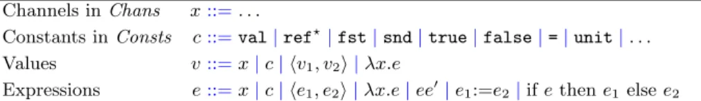
Values and Expressions. An attribute language over Chans is a triple L = (Consts, Succ, ⇓). It defines a call-by-value lambda calculus, whose values v ∈
Vals and expressions e ∈ Exprs are given in Fig. 1. Besides the usual concept of
variables x ∈ Chans, abstractions λx.e, and applications, there are expressions
e1:=e2 for imperative assignments. Additionally, we assume function constants
val, ref! ∈ Consts in order to access values of variables in the environment.
Furthermore, we include pairs #e1, e2$ with selectors fst, snd and conditionals
if e then e1else e2 with Boolean constants true, false ∈ Consts. Equality tests
on constants are provided by a constant = of type Consts × Consts → B. There may be many further constants in Consts such as for arithmetics. As usual, we write fn(e) and bn(e) for the sets of free and bound variables in e. We use infix syntax without extra notice, for instance, writing e1=e2instead of = #e1, en$. The
shortcuts in Fig. 2 provide let expressions, sequential composition, conditionals without else, and simple pattern matching functions.
An environment for an expression e ∈ Exprs is a total function ρ : fn(e) →
Vals that maps free variables of e to values. We write dom(ρ) = fn(e) for the
Channels in Chans x::=. . .
Constants in Consts c::=val|ref!|fst|snd|true|false|=|unit|. . .
Values v::=x|c|!v1, v2"|λx.e
Expressions e::=x|c|!e1, e2"|λx.e|ee!|e1:=e2|if e then e1 else e2 Fig. 1. Values and expressions of the imperative call-by-value lambda calculus. let x = e1 in e2 =df (λx.e2)e1 if e then e1 =df if e then e1 else false
e1; e2 =df let = e1 in e2 if not e then e1 =df if e then false else e1
λ!c, x".e =df λp. if (fst p)=c then (λx.e)(snd p)
Fig. 2. Shortcuts for expressions
domain of ρ and let Env be the set of all environments for arbitrary expressions. We write ρ[x1'→ v1, . . . , xn → vn] for the environment that maps distinct
vari-able xi to vi for all 1 ≤ i ≤ n and all other variables y in the domain of ρ to
ρ(y). Environments such as [x'→ #x, y$, y '→ #x, x$] can store any type of data
structure, including graphs and hypergraphs. In a stochastic setting, they are useful to assign rates to reactions.
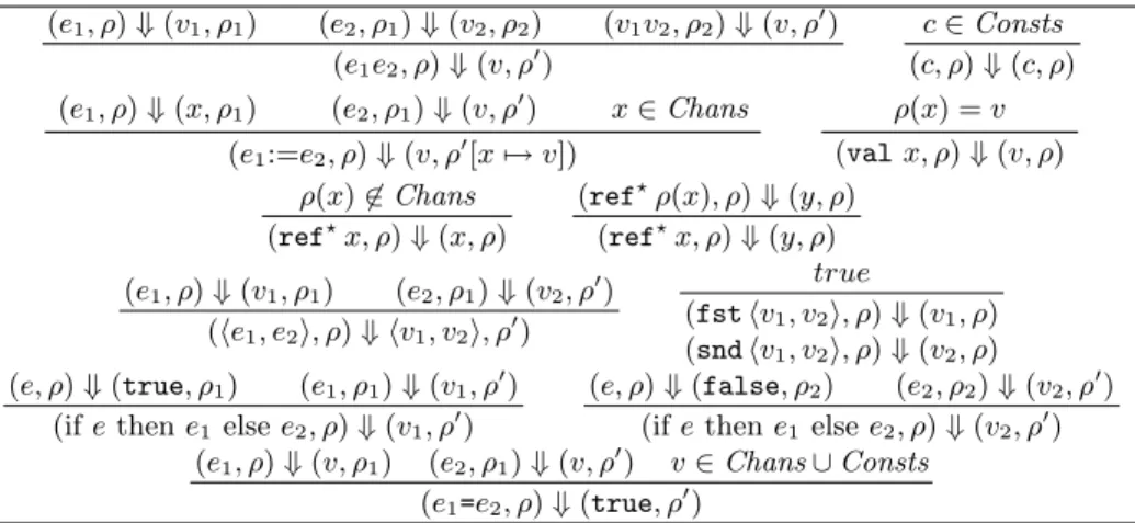
The third component of L, the big-step evaluator ⇓, is a binary relation of type (Exprs × Env) × (Vals × Env). It fixes the semantics of all expressions. A relationship (e, ρ) ⇓ (v, ρ!) states that expression e in environment ρ evaluates to
value v with new environment ρ!. The big-step evaluator must satisfy the rules in
Fig. 3. Assignments x:=v change the value of x in the current environment to v. Function val returns the value of a channel in the current environment. Function ref!serves for dereferentiation, i.e. it returns the last channel of acyclic reference
chains. In the environment [x1 '→ x2, . . . , xn−1 '→ xn, xn '→ v], (ref!xi) e.g.
evaluates to xn for all 1 ≤ i ≤ n if v )∈ Chans, while evaluation does not
terminate if v = xn.
The second component of L is a subset Succ ⊆ Vals. We call the elements of Succ successful values. Their role in πimp(L) is to describe the rate constants
of communication actions. Considering a stochastic semantics, Succ equals R+.
Otherwise, it typically contains true but not false.
Processes. The syntax of πimp(L), as given in Fig. 4, is equal to that of the
attributed π-calculus [11], except that we now permit imperative assignments in L. It extends on the usual syntax of the stochastic π-calculus [17, 16, 13], by permitting expressions to describe channel values, adding conditions to receivers and senders, and generalizing stochastic rate constants of channels to arbitrary values.
We assume a set of process names ranged over by A, each with a fixed arity
ar(A)≥ 0. Furthermore, we freely use sequence notion, writing ˜e for a sequence
of expressions, ˜x and ˜y for a sequence of channels, and ˜v for a sequence of values. Their lengths are denoted by |˜e|, |˜v|, and |˜x|, respectively.
A program consists of an initial process P0 and a set of process definitions
{D1, . . . , Dn}, exactly one per process name in P0. A definition D of A has the
(e1, ρ)⇓ (v1, ρ1) (e2, ρ1)⇓ (v2, ρ2) (v1v2, ρ2)⇓ (v, ρ!) (e1e2, ρ)⇓ (v, ρ!) c∈ Consts (c, ρ)⇓ (c, ρ) (e1, ρ)⇓ (x, ρ1) (e2, ρ1)⇓ (v, ρ!) x∈ Chans (e1:=e2, ρ)⇓ (v, ρ![x%→ v]) ρ(x) = v (val x, ρ)⇓ (v, ρ) ρ(x)'∈ Chans (ref!x, ρ)⇓ (x, ρ) (ref!ρ(x), ρ) ⇓ (y, ρ) (ref!x, ρ)⇓ (y, ρ) (e1, ρ)⇓ (v1, ρ1) (e2, ρ1)⇓ (v2, ρ!) (!e1, e2", ρ) ⇓ !v1, v2", ρ!) true (fst!v1, v2", ρ) ⇓ (v1, ρ) (snd!v1, v2", ρ) ⇓ (v2, ρ) (e, ρ)⇓ (true, ρ1) (e1, ρ1)⇓ (v1, ρ!)
(if e then e1 else e2, ρ)⇓ (v1, ρ!)
(e, ρ)⇓ (false, ρ2) (e2, ρ2)⇓ (v2, ρ!) (if e then e1else e2, ρ)⇓ (v2, ρ!) (e1, ρ)⇓ (v, ρ1) (e2, ρ1)⇓ (v, ρ!) v∈ Chans ∪ Consts
(e1=e2, ρ)⇓ (true, ρ!)
Fig. 3. Big-step evaluator for call-by-value lambda calculus.
form A(˜x) ! P, where P is a process and |˜x| = ar(A). Process P is a parallel composition of sums, channel creators, and defined processes. A channel creator (νx:v) P asks for the creation of a new channel x with scope P that is mapped to
v by the global environment. A sender v[e]!˜v, which conveys a sequence of values
˜v on channel v, is constrained by expression e. A receiver v[e]?˜y of a sequence of values for parameters ˜y on channel v is conditioned by expression e. A call of a defined process A(˜e) consists of a process name A and a sequence ˜e ∈ Exprs where |˜e| = ar(A). A sum Σ offers a choice π1.P1+ . . . + πn.Pn between senders
or receivers πi.Pi, i.e., where πiit either a sender or receiver prefix.
Nondeterministic Operational Semantics. We start with a nondetermin-istic operational semantics for πimp(L) with an arbitrary attribute language L.
The sets of free and bound names of processes fn(P ) and bn(P ) are defined as usual, except that free and bound names in expressions are to be considered too. The usual structural congruence on π-calculus processes P ≡ P!is the least
con-gruence containing alpha conversion P =αP!, where summation + and parallel
composition | are associative and commutative, the latter with neutral element
Processes P, Q::=A(˜e) defined process
| P1| P2 parallel composition
| (νx:v) P channel creation
| Σ sums
| 0 empty solution
Sums Σ::=π.P prefixed process
| Σ + Σ! summation
Prefixes π::=v[e]?˜y receiver
| v[e]!˜v sender
Definitions D::=A(˜x)! P parametric process definition
Fig. 4. Syntax of πimp(
L): e, ˜e are expressions and v, ˜v values of L, and x, ˜x ∈ Chans.
0, and satisfy the usual scoping rules of ν-binders: (νx:v) (P1| P2) ≡ (νx:v) P1| P2 if x )∈ fn(P2)
(νx:v) (νy:v!) P ≡ (νy:v!) (νx:v) P if x )∈ fn(v!) and y )∈ fn(v)
An environment for a process P is a function ρ : fn(P ) → Vals.
The nondeterministic operational semantics in Fig. 5 defines judgements (P1, ρ1) → (P2, ρ2) meaning that a process P1 in environment ρ1 reduces in
one step to process P2 while changing the environment to ρ2. The structural
congruence may silently be applied at any point (Context). A step may either be a communication or an application of a defined process. A communication step (Com) applies to a sender and a receiver on the same channel x. Let e1
and e2 be the conditions of sender and receiver, respectively, and ρ the current
environment. The communication step is enabled if (e1e2, ρ) reduces to (v, ρ!)
for some successful value v ∈ Succ. In this case, the resulting process contin-ues in environment ρ!, which may have been altered by assignment operations
in e1e2. In practice, a big step evaluator for e1e2 may first have to change the
environment and then run into an irreducible expression (a program error) or an unsuccessful value (where the communication constraint fails). In these cases, all changes done to the environment are to be backtracked. Furthermore, it may happen that the big step evaluator does not terminate (another kind of program error). An application step (Rec) of a defined process A(˜e) evaluates all expres-sion in ˜e from the left to the right while threading the environment changes, and if successful, applies the definition of A to the resulting values ˜v. Parallel com-positions (Par) may be evaluated in arbitrary order even though the changes of the environment may depend on it. Rule (Res) for channel creation (νx:v) P in environment ρ first adds [x '→ v] to the environment, then reduces (P, ρ[x '→ v]) to some (P!, ρ![x '→ v!]), and continues with ((νx:v!) P!, ρ!) where the new value
v! of x is put back into a ν binder.
Stochastic Operational Semantics. In the stochastic operational semantics all redexes must be computed before reducing one of them. The computation of redexes requires to evaluate L expressions, which may fail with program errors or nontermination. If the computation of a single redex fails, the whole process
(e1e2, ρ)⇓ (v, ρ!) v∈ Succ (Com)
(x[e1]?˜y.P + Σ1| x[e2]!˜v.Q + Σ2, ρ)→ (P [˜v/˜y] | Q, ρ!) (˜e, ρ)⇓ (˜v, ρ!) A(˜x)! P (Rec) (A(˜e), ρ)→ (P [˜v/˜x], ρ!) (P, ρ)→ (P!, ρ!) (Par) (P | Q, ρ) → (P!| Q, ρ!) (P, ρ[x%→ v]) → (P!, ρ![x%→ v!]) x'∈ dom(ρ) ∪ dom(ρ!) (Res) ((νx:v) P, ρ)→ ((νx:v!) P!, ρ!) P ≡ P! (P!, ρ)→ (Q!, ρ!) Q!≡ Q (Context) (P, ρ)→ (Q, ρ!)
Fig. 5. Nondeterministic operational semantics.
Redexes (1≤ j ≤ m, i1, j1, i2, j2∈ N) (choose) (˜e, ρ)⇓ (˜v, ρ
!) A(˜x)! N(π
1.S1+ . . . + πm.Sm)
choosej(A(˜e), ρ) = (N (πj.Sj)[˜v/˜x], ρ!)
(redex)
choosej1(Ai1(˜ei1), ρ) =α(S1!, ρ1) S1! = (νy!1:v1) (x[e!1]?˜y.S1)
choosej2(Ai2(˜ei2), ρ1) =α(S2!, ρ!) S2! = (νy!2:v2) (x[e!2]!˜v.S2) i1'= i2 (S!1, S!2, ρ!)∈ redex(i1,j1,i2,j2)(Qni=1Ai(˜ei), ρ)
where x∈ Chans, x '∈ { ˜y1} ∪ { ˜y2} and { ˜y1} ∩ { ˜y2} = ∅. Labeled reduction (r∈ R+ and & = (i
1, j1, i2, j2)∈ N4)
(com)
(N1(x[e!1]?˜y.S1), N2(x[e!2]!˜v.S2), ρ1)∈redex#(Qni=1Ai(˜ei), ρ)
(e!1e!2, ρ1)⇓ (r, ρ!) r∈ Succ (Qni=1Ai(˜ei), ρ) r − → # ( Qn
i=1,i"=i1,i2Ai(˜ei)| N1N2(S1[˜v/˜y] | S2), ρ
!) (new) (S, ρ[v/x]) r −→ # (S !, ρ![v!/x]) x'∈ dom(ρ) ∪ dom(ρ!) ((νx:v) S, ρ)−→r # ((νx:v !) S!, ρ!) Markov chain (r, r!∈ R+) (conv) ∀&∈N4
∀(N1(x[e!1]?˜y.S1), N2(x[e!2]!˜v.S2))∈ redex#(S, ρ) ∃v∈Vals∃ρ!: (e! 1e!2, ρ)⇓ (v, ρ!) (S, ρ)⇓ (sum) (S, ρ)⇓ S≡ S1 r =P {#|(S1,ρ)−→r! ! (S2,ρ!) and S2≡S!} r! r'= 0 (S, ρ)−→ (Sr !, ρ!)
Fig. 6. Stochastic operational semantics.
is considered erroneous. In any case, all state changes during redex computation need to be backtracked before verifying the next redex candidate. Only the finally selected redex is permitted to definitely commit its changes to the environment. The stochastic semantics in Fig. 6 applies to programs in biochemical form and preserves these forms by reduction. A solution S is a process in biochemical
form NΠm
i=1Ai(˜ei), where N is a quantifier prefix (νx1:v1) . . . (νxn:vn) and
Πm
i=1Ai(˜ei) = A1(˜e1) | . . . | An(˜em) a parallel composition of so called molecules.
Molecules Ai(˜ei) must have definitions in biochemical form Ai(˜xi)! NiΣiwhere
Σi is a sum of prefixed processes in biochemical form. See Appendix B for a
formal definition of processes in biochemical form. As usual, all process can be brought into biochemical form by flattening out nested sums into intermediate definitions.
The stochastic semantics of a program in biochemical normal form is a Markov chain, whose states are pairs ([S]≡, ρ), where [S]≡ is a class of a
so-lution S wrt. structural congruence ≡, and ρ is an environment for S. In order to compute a transition for such pairs, we need to compute all potential re-ductions of (S, ρ) and sum up their stochastic rates (sum). The computation of all redexes must converge (conv) before applying any reduction step. A label
' = (i1, j1, i2, j2) ∈ N4 fixes the j1’th alternative of molecules Ai1(˜ei1) of S and
the j2’th alternative of molecule Ai2(˜ei2). Label ' distinguishes a redex candidate
if these molecules have distinct indexes i1 )= i2, and if the selected alternatives
consist of a sender and a receiver on the same channel (redex). Label ' defines a
redex, if the sequences of expressions ˜e1and ˜e2can be evaluated successfully from
left to right (choose), while starting with environment ρ, threading changes, and ending in some environment ρ!. In this case, we can apply the definitions
of Ai1 and Ai2 to the resulting values, and instantiate the alternatives with
in-dex j1 and j2 to S1! and S2! . Note that the triple (S1!, S2!, ρ!) ∈ redex#(S, ρ) is
unique up to alpha renaming. Rule (com) performs the actual communication step for a redex with label ' under the condition that the constraint of the redex is successful. Rule (new) is as for the nondeterministic case.
Consider e.g. a solution A(x:=1) | B(x:=2). The evaluation order for the two assignments may vary with the redex candidate. For candidates where A(x:=1) provides the receiver and B(x:=2) the sender, we have to evaluate x:=1 before
x:=2, so that we have to test the communication constraint with store [x'→ 2].
In the symmetric case, we will have to evaluate in the opposite order and to test the constraint with store [x '→ 1].
Stochastic Simulation.A stochastic simulator for πimp(L) can be derived from
the stochastic operational semantics independently of L. The main difference to the attributed π-calculus [11] is the treatment of imperative expressions, which can either occur in constraints or in applications. Assignments in constraints in-crease computational complexity, since they force us to not only compare values but also environments for grouping senders and receivers. Furthermore, senders and receivers can not be evaluated separately anymore, but only in combina-tion. However, computational complexity can be reduced by storing differences between environments before and after evaluation, i.e. the set of executed assign-ments, since then only the latter need to be compared. Assignments in applica-tions make the extraction of multisets from soluapplica-tions less effective and therefore negatively affect simulation efficiency. More details are given in Appendix C.
3
A Model of Osmosis: Variable Volumes and Surfaces
Osmosis is a simple example for concurrent systems with compartments of vari-able volumes. It was modeled already in [21] based on a special purpose dialect
Sπ@ of π@ with variable volumes. Here we show how to simulate osmosis in the
imperative π-calculus with an attribute language that provides arithmetics. Our solution is more flexible and accurate, in that it accounts for dynamic changes of compartment surfaces, which cannot be expressed in Sπ@.
We consider a very simple system which consists of a sphere filled with water (H2O), sodium (Na+), and chlorine (Cl−). The system contains a membrane
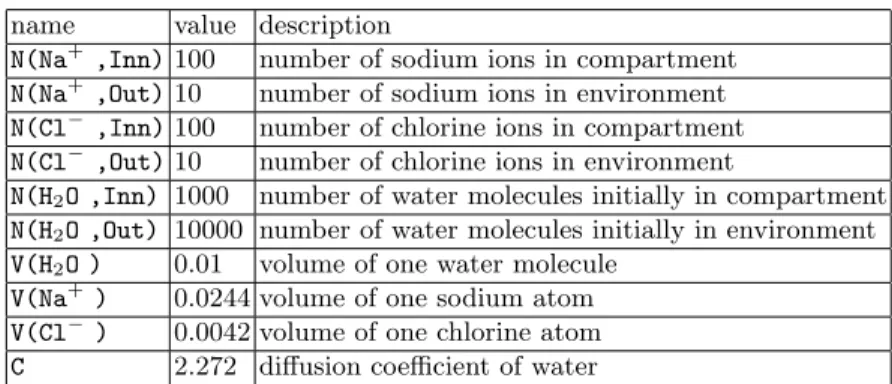
through which water may diffuse. This membrane separates an inner compart-ment Inn of spherical shape, from an outer compartcompart-ment Out, which has the form of a sphere shell (a ring in 2D). The center point equals for both compartments. The precise values of all parameters are given in Table 1.
Parameters
N : {H20 , Na+, C l−}×{ Inn , Out} → N // copy numbers o f m o l e c u l e s Constants V : {H20 , Na+, C l−} → R+ // m o l e c u l e v o l u m e s C ∈ R // d i f f u s i o n c o e f f i c i e n t o f w a t e r E x p r e s s i o n s rad =df λv . ( ( 3∗ v ) /(4∗π ) ) 1 3 // volume t o r a d i u s surf =df λ r . 4∗ π∗ r2 // r a d i u s t o s u r f a c e dist =df λ r1λ r2. r1 + ( ( r2−r1) / 2 ) // d i f f u s i o n d i s t a n c e r =df rad (Pc∈{Inn,Out} P m∈{H20,Na+,CL−}V(m)∗N(m, c ) ) // o u t e r r a d i u s o f // s p h e r e s h e l l P u b l i c c h a n n e l s // i n i t i a l i z e v o l u m e s o f compartments i n n : Pm∈{H20,Na+,CL−} V(m)∗N(m, I n n ) // i n n e r s p h e r e o u t : Pm∈{H20,Na+,CL−} V(m)∗N(m, Out ) // o u t e r s p h e r e s h e l l d i f f u s e : u n i t // d i f f u s i o n c h a n n e l P r o c e s s d e f i n i t i o n s H2O( o r i , d e s ) ! d i f f u s e [ λ . let // d i f f u s i o n from o r i g i n t o d e s t i n a t i o n r = rad ( v a l i n n ) // r a d i u s o f i n n e r s p h e r e a = ( surf r ) /10 // d i f f u s i o n a r e a s = dist r r // d i f f u s i o n d i s t a n c e d i f f = a∗C/( s ∗( v a l o r i ) ) // d i f f u s i o n r a t e in o r i := v a l o r i − V(H2O) ; // u p d a t e volume o f o r i g i n d e s := v a l d e s + V(H2O) ; // u p d a t e volume o f d e s t i n a t i o n d i f f // r e t u r n d i f f u s i o n r a t e ] ? ( ) . H2O( des , o r i )
Membrane ( ) ! d i f f u s e [ unit ] ! ( ) . Membrane ( ) S o l u t i o n
QN(H2O,Inn)
i=1 H2O( i n n , o u t ) |
QN(H2O,Out)
i=1 H2O( out , i n n ) | Membrane ( )
Fig. 7. Modeling osmosis
For simplicity, we adopt the assumption of [21], that the volume of a com-partment is determined by summing up the volumes of the contained molecules. However, in general, L allows for the definition of complex functions to obtain compartment volumes that e.g. consider atomic forces between particles. The volumes of Inn and Out change with water moving through the membrane. The radius of Inn may thus vary with diffusion, while the outer radius r of Out always remains fixed. Fig. 7 shows our model of the system in πimp(L(R, V, C)).
Its attribute language provides real number arithmetics with function constants for division /, multiplication *, and subtraction -, and numeric constants such as 2, 10, or π. Furthermore, there are three problem specific constants, the dif-fusion coefficient C of H2O, the constant V for the function that maps molecules
to their volumes, and the constant N for the function assigning copy numbers to
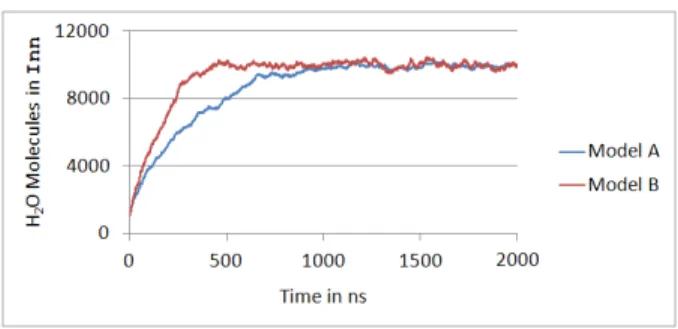
Fig. 8. Experiment results without (Model A) and with (Model B) variable surfaces.
molecules in compartments. The big-step evaluator for L(R, V, C) is defined as usual. Nonzero positive real numbers are successful, Succ = R+.
The diffusion rate of H2O is determined by a∗Cd∗v, where a is the diffusion area,
d the diffusion distance, and v the volume of the compartment that the molecule
leaves, see [8]. We assume that 1/10 of Inn’s surface serves as diffusion area. The radius and surface of Inn are computed from its volume by functions rad and surf, see Fig. 7. The diffusion distance represents the average way a molecule travels from one compartment to the other. Following the approach in [8], we assume the diffusion distance to be the distance between the two compartment centers. In the model, it is determined by function dist applied to the constant outer radius of Out and the variable radius of Inn.
In our model, we represent the compartments Inn and Out as public chan-nels inn and out, respectively, each referring to the variable volume of the corre-sponding compartment. The public channel diffuse with the dummy value unit represents diffusion reactions. Three processes are defined: H2O(inn,out), which
describes a water molecule in Inn that may diffuse to Out, H2O (out,inn), its
symmetric variant, and Membrane(), which enables diffusion on channel diffuse at all times.
The parametric processes H2O (ori,des) may perform diffusion by
commu-nication on channel diffuse and then continue with H2O(des,ori). The speed
of this reaction is given by the diffusion rate, which varies with volumes and surfaces and is therefore consecutively recomputed. This is done by applying the function in the brackets diffuse[...]?. Every application of this function per-forms volume changes by assignments ori := val ori - V(H2O ) and des :=
val ori + V(H2O ). Since the simulator needs to compute the diffusion rates for
all possible interactions in the system (there are at most two, water moving in or out), it has to reset the environment every time. Only once some interaction is chosen by the Stochastic Simulation Algorithm [9], it can commit to the changes required by this interaction.
By adapting the diffusion area and distance at each diffusion event, we extend the model presented in [21], where only volume changes are considered. In order to compare both versions of the model, we implemented and simulated them in our tool, which is part of the modeling and simulation framework JamesII [10].
The results can be seen in Fig. 3. Model B, being the one that considers updates of the diffusion area and distance, features a steeper slope. This is due to the fact that with the increasing volume of Inn, the diffusion area grows faster than the distance, which raises the resulting diffusion rates.
4
Programming BioAmbients
We encode BioAmbients [18] in the imperative π-calculus, in order to show how to express concurrent systems with compartments and dynamic rearrangement systematically. In a first step, we ignore local stochastic aspects as in [1, 15] which would not impose any particular problem, since these do not account for volume changes. See below for a discussion of extensions.
The syntax of BioAmbients is recalled in Fig. 9. It has the same syntac-tic categories as the π-calculus. Processes P can be enclosed by ambients [P ] whose nesting structure restricts interaction capacities similarly to compart-ments. There are prefixes for two kinds of interactions: communication and re-arrangement. Communication prefixes ”d x?(˜y)” and ”d x!(˜y)” are prefixes of senders or receivers annotated by a communication direction d, which is either local, s2s, c2p, or p2c. They enable message sending either locally in an ambi-ent, between sibling ambients, from a parent to a child, or vice versa. Similarly, there are rearrangement prefixes, prefixes of senders ”c x!” and receivers ”c x?” without arguments and annotated by rearrangement capacity c, either merge, in, or out. Rearrangement operations with these prefixes serve for ambient merging, entering into siblings, or exiting the current ambient. The reduction rules of the (nondeterministic) operational semantics of BioAmbients are given in Fig. 10. We refer the reader to [18] for the full operational semantics.
In order to encode BioAmbients, we identify every ambient using a channel
r that gives reference to the characteristic values (cv) of the ambient. The cv #n, r!$ consists of a unique name n naming the ambient and the reference r!of its
parent (which is unit at the top-level). The ambient is encoded by a store binding
r to the cv possibly via a reference chain: [r'→ r1, . . . , rn−1'→ rn, rn'→ #n, r!$].
The elements in ambient r will be encoded by defined processes A(r).
Characteristic values can be changed by assignments r:=v. When assign-ments are executed, the simulation algorithm automatically updates the com-munication potential of all elements in the compartment. For instance, for a compartment that contains n copies of the same element A(r), all updates can
Processes P, Q::=[P ]|A(˜x)|P|Q|(νx:v) P|Σ|0
Sums Σ, Σ!::=π.P | Σ + Σ!
Prefixes π::=d x!˜z|d x?˜z|c x!|c x?
Communication directions d::=local|s2s|c2p|p2c
Rearrangment capacities c::=merge|in|out
Definitions D::=A(˜x)! P
Fig. 9. Syntax of BioAmbients
Communication : local x!˜z.P + Σ| local x?˜y.Q + Σ! → P | Q{˜z/˜y} ˆ Q| c2p x!˜z.P + Σ˜| c2p x?˜y.P!+ Σ! → [Q | P ] | P!{˜z/˜y} ˆ Q| p2c x?˜y.P + Σ˜| p2c x!˜z.P!+ Σ! → ˆQ| P {˜z/˜y}˜| P! ˆ Q| s2s x!˜z.P + Σ˜|ˆQ!| s2s x?˜y.P!+ Σ!˜ → [P | Q] |ˆQ!| P!{˜z/˜y}˜ Rearrangement : [Q| merge x!P + Σ] | [Q!| merge x?P!+ Σ!] → [Q | P | Q!| P!]
[Q| in x!P + Σ] | [Q!| in x?P!+ Σ!] → ˆ[Q| P ] | Q!| P!˜
ˆ
[Q| out x!P + Σ] | Q!| out x?P!+ Σ!˜ → [Q | P ] | [Q!| P!]
Fig. 10. Reduction rules of BioAmbients
be done by a single inspection of the definition of A(r), not n-times in contrast to priority-based encodings. Since dereferentiation might be required, this might still cost time O(n) in the rare worst case, but will often be more efficient.
We encode BioAmbients into πimp(L(cap, dir)), which provides constants for
all directions and capacities of BioAmbients. The encoding is given in Fig. 12.
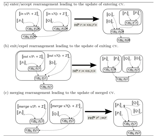
(a) enter/accept rearrangement leading to the update of entering cv.
(b) exit/expel rearrangement leading to the update of exiting cv.
(c) merging rearrangement leading to the update of merged cv.
Fig. 11. Simplified diagrams illustrating enter, exit and merge rearrangements.
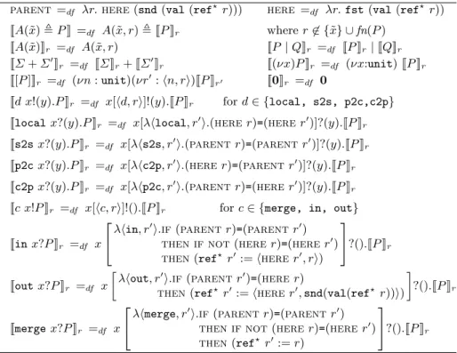
parent =df λr. here (snd (val (ref!r))) here =df λr. fst (val (ref!r))
!A(˜x) ! P " =df A(˜x, r)! !P "r where r'∈ {˜x} ∪ fn(P )
!A(˜x)"r =df A(˜x, r) !P | Q"r =df !P "r| !Q"r
!Σ + Σ!"r =df !Σ"r+!Σ!"r !(νx)P "r =df (νx:unit)!P "r
![P ]"r =df (νn : unit)(νr!:!n, r")!P "r! !0"r =df 0
!d x!(y).P "r =df x[!d, r"]!(y).!P "r for d∈ {local, s2s, p2c,c2p}
!local x?(y).P "r =df x[λ!local, r!".(here r)=(here r!)]?(y).!P "r
!s2s x?(y).P "r =df x[λ!s2s, r!".(parent r)=(parent r!)]?(y).!P "r
!p2c x?(y).P "r =df x[λ!c2p, r!".(here r)=(parent r!)]?(y).!P "r
!c2p x?(y).P "r =df x[λ!p2c, r!".(parent r)=(here r!)]?(y).!P "r
!c x!P "r =df x[!c, r"]!().!P "r for c∈ {merge, in, out}
!in x?P "r =df x
2 4λ!in, r
!".if (parent r)=(parent r!)
then if not (here r)=(here r!) then (ref!r!:=!here r!, r")
3 5?().!P "r
!out x?P "r =df x
»
λ!out, r!".if (parent r!)=(here r)
then (ref!r!:=!here r!, snd(val(ref! r)) ") – ?().!P "r !merge x?P "r =df x 2 4λ!merge, r
!".if (parent r)=(parent r!)
then if not (here r)=(here r!) then (ref!r!:= r)
3 5?().!P "r
Fig. 12. Encoding BioAmbients
We first define two lambda expressions here and parent which map ambients r to their name here r = n and to the name of their parent parent r = here r!.
For every BioAmbients process P in ambient r, the encoding defines a unique process !P "r in πimp(cap, dir). Encoding an ambient [P ] with parent r consists
in creating a new ambient name n and a reference r!to the cv #n, r$, and proceed
with the encoding !P "r!. In general, this is how one can dynamically create new ambients. Encodings of rearrangement prefixes are illustrated by the diagrams in Fig. 11. Dashed arrows link references to their cv’s. The graphical boxes represent ambients [P ] and are annotated by the cv of the ambient.
In Diagram (a), ambient r with cv #n1, r1$ enters ambient r!with cv #n2, r2$.
The translation has to specify that the first ambient becomes a child of the second. Therefore, we update the cv of r to #n1, r!$, such that its parent is now
r!. Note that the rearrangement is allowed only if the ambients are siblings. We
thus have to perform the sibling test and the cv update in an atomic manner by a communication constraint on x in !in x?P "r:
λ#in, r!$.if (parent r)=(parent r!) then
if not (here r)=(here r!) then (ref! r!) := #here r!, r$
This function matches its argument against the pair #in, r!$, checks that the
parent of receiver r coincides with the parent of its communication partner r!,
checks that both processes are not located within the same ambient and finally updates the cv of the sender accordingly. Note that an encoding of BioAmbients with stochastic aspects, as considered in [1, 15], would simply make this function return the rate of x (that is val x assuming communication channels refer to their stochastic rate) in the sequence with the reference assignment. Diagram (b) describes the exiting ambients and Diagram (c) ambient merging. These used similar concepts as ambient entering in Diagram (a).
We define the top-level encoding !P "νrby (νr:#unit, unit$) !P "rand call an
environment ρ for P ground if ρ(x) = unit for all x ∈ fn(P ). We define - as the least congruence such that ≡⊆- and (νr!:v) (νr:r!) P - (νr!:v) P {r!/r
}. This
equivalence is preserved by reduction of BioAmbients encodings, that is for any BioAmbients term P and πimp(L(cap, dir)) processes Q
1= !P "νr and Q2, such
that Q1- Q2, then (Q1, ρ)→ (Q!1, ρ) iff (Q2, ρ)→ (Q!2, ρ) with Q!1- Q!2.
Theorem 1 (Soundness and completeness of BioAmbients encoding).
1. For all BioAmbients processes P, P!, if P → P! then there exists a process
Q! - !P!"
νr of πimp(L(cap, dir)) such that (!P "νr, ρ) → (Q!, ρ) for every
ground environment ρ of !P "νr.
2. For all BioAmbients processes P , ground environment ρ of !P "νr, and
πimp(L(cap, dir)) process Q!, if (!P "νr, ρ) → (Q!, ρ) then there exists a
BioAmbients process P! of such that P → P! and !P!"
νr - Q!.
BioAmbients with Variable Volumes. Stochastic rates of reactions in com-partmented systems depend on concentrations of reactants and thus on volumes of compartments. This was already illustrated by the osmosis example in Section 3. In this section, we discuss notions of volumes for ambients, and how to model them in the imperative π-calculus. Which logics for volumes to choose depends on the concrete geometry that is assumed.
When considering spatial systems where compartment nesting corresponds to geometrical nesting, we have to distinguish two notions of volumes: the molecular
volume of a compartment, which sums up the volumes of all molecules that it
contains, and the geometric volume, which adds the geometric volumes of all child compartments to the molecular volume. In the osmosis example, the geometric volume of the outer sphere shell (of which is outer radius R depends) does indeed include the volumes of all molecules of the inner sphere.
In order to model BioAmbients with molecular and geometric volumes in the imperative π-calculus, we can enrich the cv’s of compartments by these volumes, and define lambda expressions mvol r and avol r to access them when know-ing the ambient’s reference r. Furthermore, we have to update these volumes for all operations of the calculus, which can be expressed by using assignment operations and real arithmetics. These details need elaboration beyond 15 pages.
5
Conclusion & Outlook
We have shown that imperative assignments for the π-calculus yield global ef-fects, that offer an alternative to priorities. These permit to express operations
of compartment dissolution and merging in an efficient, simpler and stochastic manner. The imperative π-calculus thus answers the question for a better mod-eling language for dynamic compartments. In work, we would like to further investigate on the relation to Bigraphs.
References
1. L Brodo, P Degano, and C Priami. A stochastic semantics for bioambients. In
Parallel Computing Technologies, 4671 of LNCS, 22–34. 2007.
2. L Cardelli. Brane calculi. In CMSB’04, 3082 of LNCS, 257–278 2005.
3. N Chabrier-Rivier, F Fages, and S Soliman. The Biochemical Abstract Machine BIOCHAM. In CMSB’04, 3082 of LNCS, 172–191, 2004.
4. F Ciocchetta and J Hillston. Bio-PEPA: An Extension of the Process Algebra PEPA for Biochemical Networks. ENTCS, 194(3):103–117, 2008.
5. F Ciocchetta and M L Guerriero. Modelling Biological Compartments in Bio-PEPA. In ENTCS, 227:77–95, 2009.
6. V Danos and C Laneve. Formal molecular biology. TCS, 325(1):69–110, 2004. 7. L Dematt´e, C Priami, and A Romanel. Modelling and Simulation of Biological
Processes in BlenX. SIGMETRICS Perf. Evaluation Review, 35(4):32–39, 2008. 8. J Elf and M Ehrenberg. Spontaneous Separation of Bi-Stable Biochemical Systems
into Spatial Domains of Opposite Phases. Systems Biology, IEEE Proceedings, 1(2):230–236, 2004.
9. DT Gillespie. Exact Stochastic Simulation of Coupled Chemical Reactions. Journal
of Physical Chemistry, 81:2340–2361, 1977.
10. J Himmelspach and AM Uhrmacher. Plug’n Simulate. ANSS’07, IEEE
Proceed-ings, 0:137–143, 2007.
11. M John, C Lhoussaine, J Niehren, and A Uhrmacher. The Attributed Pi Calculus. In CMSB’08, 5307 of LNCS, 83–102, 2008.
12. J Krivine, R Milner, and A Troina. Stochastic bigraphs. ENTCS, 218:73–96, 2008. 13. C Kuttler, C Lhoussaine, and J Niehren. A Stochastic Pi-Calculus for Concurrent
Objects. In Algebraic Biology, 4545 of LNCS, 232–246. 2007.
14. R Milner. Pure bigraphs: Structure and dynamics. Information and Computation, 204(1):60–122, 2006.
15. A Phillips. An Abstract Machine for the Stochastic Bioambient Calculus. ENTCS, 227:143–159, 2009.
16. A Phillips and L Cardelli. Efficient, Correct Simulation of Biological Processes in the Stochastic Pi-Calculus. In CMSB’07, 4695 of LNCS, 184–199, 2007.
17. C Priami, A Regev, E Shapiro, and W Silverman. Application of a Stochastic Name-Passing Calculus to Representation and Simulation of Molecular Processes.
Information Processing Letters, 80:25–31, 2001.
18. A Regev, EM Panina, W Silverman, L Cardelli, and E Shapiro. BioAmbients: An Abstraction for Biological Compartments. TCS, 325(1):141–167, 2004.
19. A Regev and E Shapiro. Cells as Computation. Nature, 419:343, 2002.
20. C Versari. A Core Calculus for a Comparative Analysis of Bio-Inspired Calculi. In
ESOP’07, 4421 of LNCS, 411–425, 2007.
21. C Versari and N Busi. Stochastic Biological Modelling in Presence of Multiple Compartments. TCS, to appear.
A
Parameters and Constants for Osmosis Model
name value description
N(Na+ ,Inn)100 number of sodium ions in compartment
N(Na+ ,Out)10 number of sodium ions in environment
N(Cl−,Inn)100 number of chlorine ions in compartment
N(Cl−,Out)10 number of chlorine ions in environment
N(H2O ,Inn) 1000 number of water molecules initially in compartment N(H2O ,Out) 10000 number of water molecules initially in environment
V(H2O ) 0.01 volume of one water molecule
V(Na+ ) 0.0244 volume of one sodium atom
V(Cl−) 0.0042 volume of one chlorine atom
C 2.272 diffusion coefficient of water
Table 1. Parameters and constants used in osmosis experiments
B
Completion of Standard Definitions for π
imp(
L)
Free names
fn(π1.P1+ . . . + πn.Pn) = !i∈{1,...,n}fn(πi.Pi) fn(0) = ∅
fn(v[e]?˜y.P ) = fn(v) ∪ fn(e) ∪ (fn(P ) \ {˜y}) fn(P1| P2) = fn(P1) ∪ fn(P2)
fn(v[e]!˜v.P ) = fn(v) ∪ fn(˜v) ∪ fn(e) ∪ fn(P ) fn(A(˜e)) = fn(e)
fn((νx:v) P ) = (fn(P ) ∪ fn(v)) \ {x} fn(A(˜x)! P) = fn(P) \ {x}
Biochemical normal form The stochastic semantics in Section 2 applies to processes in biochemical form which have the following abstract syntax.
Solutions S::=A(˜e) defined molecule
| S1| S2 parallel composition
| (νx:v) S channel creation
| 0 empty solution
Molecules M ::=π1.S1+ . . . + πn.Sn sum of alternative choices
| (νx:v) M channel creation
Prefixes π::=v[e]?˜y receiver
| v[e]!˜v sender
Definitions D::=A(˜x)! M molecule definition
All processes can be brought into this form, by unnesting sums into new defini-tions of parametric processes.
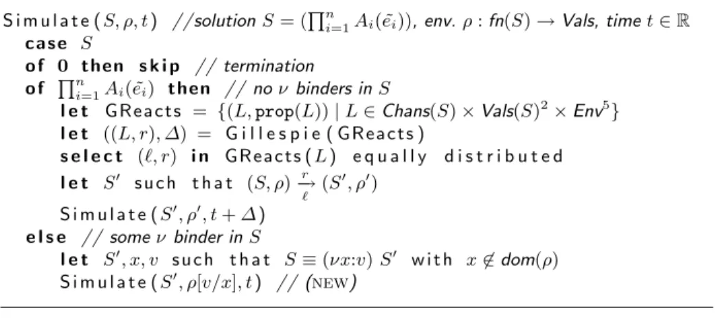
S i m u l a t e ( S, ρ, t ) //solution S = (Qni=1Ai( ˜ei)), env. ρ : fn(S)→ Vals, time t ∈ R
c a s e S
o f 0 then s k i p // termination
o f Qni=1Ai( ˜ei) then // no ν binders in S
l e t GReacts = {(L, prop(L)) | L ∈ Chans(S) × Vals(S)2
× Env5 } l e t ((L, r), ∆) = G i l l e s p i e ( GReacts ) s e l e c t (&, r) i n GReacts ( L ) e q u a l l y d i s t r i b u t e d l e t S! s u c h t h a t (S, ρ) r − → # (S !, ρ!) S i m u l a t e ( S!, ρ!, t + ∆ ) e l s e // some ν binder in S l e t S!, x, v s u c h t h a t S≡ (νx:v) S! w i t h x'∈ dom(ρ) S i m u l a t e ( S!, ρ[v/x], t ) // (new)
Fig. 13. Stochastic simulator for πimp( L)
C
Stochastic Simulator
The stochastic simulator for πimp(L) can be derived from the stochastic
semantics of πimp(L), as presented in Section 2, and defined independently of
the choice of L, see Figure 13. The input of the simulator is a pair (S, ρ, t), where S is a solution N "n
i=1Ai( ˜ei) in some environment ρ ∈ Env at time
t ∈ R. In contrast to the stochastic semantics, the simulator does not keep
possible ν binders in N, but only adds new channels with their values to the environment, which simplifies the implementation. If required, information about free names can be conserved by including an additional store. If no ν binder exists, the next reduction step is chosen in a memoryless stochastic manner and the sojourn time ∆ ≥ 0 in S is inferred. This enables the simu-lator to proceed with the resulting solution and environment at time point t+∆. In order to choose the next reduction step, Gillespie’s Stochastic Simulation Algorithm (SSA) [9] is applied to the set of labeled reactions as usual in the stochastic π-calculus, see e.e. [11]. Computing the set of labeled reactions, how-ever, is the crucial step in the simulator. A naive approach would evaluate all combinations of possible sender and receivers, which yields quadratic computa-tional complexity. A more efficient solution is to group reactions by their chan-nels, rates and environments. Therefore, we define a label for a grouped reaction in a solution S as a tuple L ∈ Chans(S)×Vals(S)2
×Env5. Thereby, L represents
the following set of reactions with respect to the solution S = ("n
i=1Ai( ˜ei), ρ): Reacts(L) = {(', r) ∈ Reacts | L = (x, v1, v2, ρ1, ρ2, ρ3, ρ4), ' = (i1, j1, i2, j2), choosej1(Ai1( ˜ei1), ρ) = (x[e]? . . . , ρ1), (ρ2, e)⇓ (v1, ρ3), choosej2(Ai2( ˜ei2), ρ1) = (x[e!]! . . . , ρ2), (ρ3, e!) ⇓ (v2, ρ4), i1)= i2, (ρ4, v1v2) ⇓ (r, ρ!)}
With ρ!, we account for the backtracking in the stochastic semantics, since it is
only applied, if one of the grouped reactions in Reacts(L) is performed. Notice, that, instead of considering them separately, senders and receivers need to be evaluated in combination in order to compute Reacts(L), which increases com-putation time. Furthermore, it is necessary to check equality of environments. In practice, however, efficiency can be radically increased, by storing the differences between the environments before and after evaluation, i.e. the set of executed assignments. By this, senders and receivers only need to be reevaluated, when different assignments are considered. Furthermore, the costs of checking equality of environments is reduced, since only sets of assignments need to be compared. For each grouped reaction label, its propensity prop(L) ∈ R+, i.e. its stochastic
rate, needs to be computed, which equals the sum of rates of grouped reactions.
prop(L) = #
(#,r)∈Reacts(L)
r
With this we can define the set of grouped reactions in S with respect to ρ, that forms the input for the SSA:
GReacts= {(L, prop(L)) | L ∈ Chans(S) × Vals(S)2
× Env5}
The propensities of all labels of grouped reactions of a solution S be derived from the values below, where S = "n
i=1Ai( ˜ei): in(x, v, ρ1, ρ2, ρ3, ρ4) = #{(i, j) | choosej(Ai( ˜ei), ρ1) = (x[ej]? . . . , ρ2), (ρ3, ej) ⇓ (v, ρ4)} out(x, v, ρ1, ρ2, ρ3, ρ4) = #{(i, j) | choosej(Ai( ˜ei), ρ1) = (x[ej]! . . . , ρ2), (ρ3, ej) ⇓ (v, ρ4)} mixin(x, v1, v2, ρ1, ρ2, ρ3, ρ4, ρ5) = #{(i, j1, j2) | choosej1(Ai( ˜ei), ρ1) = (x[ej1]? . . . , ρ2), (ρ3, ej1) ⇓ (v1, ρ4), choosej2(Ai( ˜ei), ρ2) = (x[ej2]! . . . , ρ3), (ρ4, ej2) ⇓ (v2, ρ5)},
Lemma 1. The propensity of solution S = ("n
i=1Ai( ˜ei)) in environment ρ is
given by prop(x, v1, v2, ρ1, ρ2, ρ3, ρ4) = (in(x, v1, ρ, ρ1, ρ2, ρ3) ∗
out(x, v2, ρ1, ρ2, ρ3, ρ4) − mixin(x, v1, v2, ρ, ρ1, ρ2, ρ3, ρ4)) ∗ r
if the solution does not contain infinite rates and (v1v2, ρ4) ⇓ (r, ρ!).
Proof. We need to show that $(#,r)∈Reacts(L)r = (in(x, v1, ρ, ρ1, ρ2, ρ3) ∗
out(x, v2, ρ1, ρ2, ρ3, ρ4) −mixin(x, v1, v2, ρ, ρ1, ρ2, ρ3, ρ4)) ∗r. Since r is constant,
this is true iff, $(#,r)∈Reacts(L)1 = in(x, v1, ρ, ρ1, ρ2, ρ3)∗out(x, v2, ρ1, ρ2, ρ3, ρ4)−
mixin(x, v1, v2, ρ, ρ1, ρ2, ρ3, ρ4). Let O(Reacts(L)) and I(Reacts(L)) be the
set of senders and receivers in Reacts(L). Then, $(#,r,ρ!)∈Reacts(L)1 =
|I(Reacts(L))| ∗ |O(Reacts(L))|. Senders and receivers in in(x, v1, ρ, ρ1, ρ2, ρ3)
and out(x, v2, ρ1, ρ2, ρ3, ρ4) are chosen as for Reacts(L), except the
ad-ditional condition i1 )= i2, which excludes communications of senders
and receivers of the same summation. These communications are con-sidered by mixin(x, v1, v2, ρ, ρ1, ρ2, ρ3, ρ4), such that in(x, v1, ρ, ρ1, ρ2, ρ3) ∗
out(x, v2, ρ1, ρ2, ρ3, ρ4) − mixin(x, v1, v2, ρ, ρ1, ρ2, ρ3, ρ4) = |I(Reacts(L))| ∗
|O(Reacts(L))| =$(#,r)∈Reacts(L)1.
Including the optimizations, which were discussed for computing the labels of grouped reactions, the difference in computational complexity between the sim-ulator of πimp(L) and the one of π(L), as presented in [11], basically depends on
the number of assignments in the model. In fact, considering a model not includ-ing any assignments, the computational complexity is the same, since senders and receivers can be evaluated separately. However, a further desirable opti-mization, where propensities are computed incrementally and not from scratch in every simulation step, causes problems. Such an implementation should ex-tract multi-sets from solutions S = "n
i=1Ai( ˜ei). This is less effective in πimp(L)
than in π(L), where solutions are given by S = "n
i=1Ai( ˜vi), which negatively
affects efficiency. A simple solution for this problem, which we chose for our cur-rent implementation, is to disallow assignments in A(e), such that expressions in
S ="ni=1Ai( ˜ei) can be evaluated instantaneously. This is reasonable, as it does
not influence our results on encoding BioAmbients. However, more sophisticated approaches are preferable and need to be investigated in future work.
D
Proof Sketch for Theorem 1
We need two aux statements where y/x stands for the substitution of y for x and P, Q are BioAmbients processes.
!P "r{y/x} =α!P {y/x}"r
P ≡ Q ⇒ ∀r ∈ Chans !P "r≡ !Q"r (†)
The proofs of these claims are straightforward. We now consider part 1. of The-orem 1:
1. If P → P! then, ∃Q! such that Q! - !P!"
νr and (!P "νr, ρ) → (Q!, ρ) for
every ground environment ρ of !P "νr.
The proof is by structural induction on derivations of P → P!. We will permit
us two more letters R, S to range over BioAmbients processes in addition to
P, Q. As an example, we consider the BioAmbients rule enter/exit in which
case Q! = !P!"
νr. We have P = [in x!P1+ Σ | Q] | [in x?R + Σ!|S], and
P!= [R | S | [P
1| Q]]. Let
ρ!= ρ[r0'→ #unit, unit$, n1'→ unit, n2'→ unit, r1'→ #n1, r0$, r2'→ #n2, r0$]
and let
e = λ#in, r1$.if (parent r1)=(parent r2) then (ref! r1:= #here r1, r2$)
One can check that
(e #in, r1$, ρ!) ⇓ (#n1, r2$, ρ![r1'→ #n1, r2$])
Thus, by rule (com), we have
(x[#in, r1$]!().!P1"r1+ !Σ"r1 | x[e]?().!R"r2+ !Σ!"r2, ρ!) → (!P1"r1 | !R"r2, ρ![r1'→ #n1, r2$])
Then, by rules (context) and (Par), we have
(x[#in, r1$]!().!P1"r1+ !Σ"r1| !Q"r1 | x[e]?().!R"r2+ !Σ!"r2 | !S"r2, ρ!) → (!P1"r1 | !Q"r1 | !R"r2 | !S"r2, ρ![r1'→ #n1, r2$])
Let N = (νr0 : #unit, unit$, n1: unit, n2 : unit, r2 : #n2, r0$, r1 : #n1, r0$) and
N! = (νr
0: #unit, unit$, n1: unit, n2: unit, r2: #n2, r0$, r1: #n1, r2$), by rule
(Res) we deduce
(N(x[#in, r1$]!().!P1"r1+ !Σ"r1 | !Q"r1 | x[e]?().!R"r2+ !Σ!"r2| !S"r2), ρ) → (N!(!P
1"r1| !Q"r1 | !R"r2 | !S"r2), ρ)
Moreover, by (†) we have (νn1: unit, r1: #n1, r2$)(!P1"r1 | !Q"r1) ≡ ![P1|Q]"r2,
thus
N!(!P
1"r1 | !Q"r1 | !R"r2 | !S"r2)
≡ (νr0: #unit, unit$, n2: unit, r2: #n2, r0$)(!R"r2 | !S"r2 | ![P1|Q]"r2) ≡ (νr0: #unit, unit$)![R | S | [P1| Q]]"r0 = ![R | S | [P1| Q]]"νr0 Finally, since by (†) N (x[#in, r1$]!().!P1"r1+ !Σ"r1 | !Q"r1 | x[e]?().!R"r2+ !Σ!"r2 | !S"r2) ≡ ![in x!P1+ Σ | Q] | [in x?R + Σ!|S]"νr0 we conclude that !P "νr0 → !P!"νro.
We illustrate the proof of part 2. of Theorem 1:
2. if (!P "νr, ρ)→ (Q!, ρ) then, ∃P! of such that P → P! and !P!"νr- Q!,
through a simple example of merging which introduces assignments indirec-tions and justifies the use of the congruence relation -. Suppose that P = [merge x!.P1] | [merge x?.P2] and let
N = (νr :#unit, unit$, n1: unit, n2: unit, r1: #n1, r$, r2: #n2, r$)
then,
!P "νr ≡ N(x[#merge, r1$]!().!P1"r1| x[e]?().!P2"r2)
with e defined as for merge accepting encoding. Then, let
N!= (νr : #unit, unit$, n1: unit, n2: unit, r2: #n2, r$)
one can easily check that !P "νr → N!(νr1: r2)(!P1"r1 | !P2"r2) and N!(νr1: r2)(!P1"r1| !P2"r2) - N!(!P1"r2 | !P2"r2) ≡ ![P1| P2]"νr
Therefore, finally,
![merge x!.P1] | [merge x?.P2]"νr →- ![P1| P2]"νr