Impact of precession on the climate, vegetation and fire activity in southern Africa during MIS4

HAL Id: hal-01312984

https://hal.sorbonne-universite.fr/hal-01312984

Submitted on 9 May 2016

HAL is a multi-disciplinary open access

archive for the deposit and dissemination of

sci-entific research documents, whether they are

pub-lished or not. The documents may come from

teaching and research institutions in France or

abroad, or from public or private research centers.

L’archive ouverte pluridisciplinaire HAL, est

destinée au dépôt et à la diffusion de documents

scientifiques de niveau recherche, publiés ou non,

émanant des établissements d’enseignement et de

recherche français ou étrangers, des laboratoires

publics ou privés.

activity in southern Africa during MIS4

M.-N Woillez, G Levavasseur, A.-L Daniau, M Kageyama, D.H. Urrego, M.-F

Sánchez-Goñi, V Hanquiez

To cite this version:

M.-N Woillez, G Levavasseur, A.-L Daniau, M Kageyama, D.H. Urrego, et al.. Impact of precession on

the climate, vegetation and fire activity in southern Africa during MIS4. Climate of the Past, European

Geosciences Union (EGU), 2014, 10 (3), pp.1165-1182. �10.5194/cp-10-1165-2014�. �hal-01312984�

www.clim-past.net/10/1165/2014/ doi:10.5194/cp-10-1165-2014

© Author(s) 2014. CC Attribution 3.0 License.

Impact of precession on the climate, vegetation and fire activity in

southern Africa during MIS4

M.-N. Woillez1,2,3, G. Levavasseur4, A.-L. Daniau1, M. Kageyama5, D. H. Urrego1,2,3, M.-F. Sánchez-Goñi2, and V. Hanquiez1

1_{Centre National de la Recherche Scientifique (CNRS), Environnements et Paléocenvironements}

Océaniques et Continentaux (EPOC), Unité Mixte de Recherche, UMR5805, CNRS – Université Bordeaux 1, 33400 Talence, France

2_{Ecole Pratique des Hautes Etudes (EPHE), EPOC, UMR 5805, 33400 Talence, France}

3_{CNRS, de la Préhistoire à l’Actuel: Culture, Environnement et Anthropologie (PACEA), UMR 5199, 33400 Talence, France}

4_{Institut Pierre Simon Laplace, Pôle de Modélisation du Climat, Université Pierre et Marie Curie, 4 Place Jussieu,}

Paris, France

5_{LSCE/IPSL INSU, UMR 8212, CE Saclay, l’Orme des Merisiers, 91191 Gif-sur-Yvette Cedex, France}

Correspondence to: M.-N. Woillez (marienoelle.woillez@gmail.com)

Received: 20 July 2013 – Published in Clim. Past Discuss.: 17 September 2013 Revised: 28 April 2014 – Accepted: 29 April 2014 – Published: 18 June 2014

Abstract. The relationships between climate, vegetation and fires are a major subject of investigation in the context of cli-mate change. In southern Africa, fire is known to play a cru-cial role in the existence of grasslands and Mediterranean-type biomes. Microcharcoal-based reconstructions of past fire activity in that region have shown a tight correlation between grass-fueled fires and the precessional cycle, with maximum fire activity during maxima of the climatic preces-sion index. These changes have been interpreted as the result of changes in fuel load in response to precipitation changes in eastern southern Africa. Here we use the general circulation model IPSL_CM5A (Institut Pierre Simon Laplace Climate Model version 5A) and the dynamic vegetation model LPJ-LMfire to investigate the response of climate, vegetation and fire activity to precession changes in southern Africa during marine isotopic stage 4 (74–59 kyr BP). We perform two cli-matic simulations, for a maximum and minimum of the pre-cession index, and use a statistical downscaling method to in-crease the spatial resolution of the IPSL_CM5A outputs over southern Africa and perform high-resolution simulations of the vegetation and fire activity. Our results show an anticorre-lation between the northern and southern African monsoons in response to precession changes. A decrease of the preces-sion climatic index leads to a precipitation decrease in the

summer rainfall area of southern Africa. The drying of cli-mate leads to a decrease of vegetation cover and fire activ-ity. Our results are in qualitative agreement with data and confirm that fire activity in southern Africa during MIS4 is mainly driven by vegetation cover.

1 Introduction

The relationships between climate, ecosystems and fire are currently a major concern in the context of future climate change, as fire risk is expected to increase in several regions worldwide in response to both the rise in temperature and precipitation decrease (Liu et al., 2010). However the studies on this issue are usually based on predicted temperature and precipitation changes only (Liu et al., 2010). They do not take into account possible shifts in the ecosystems, which would change the amount of fuel available or its composi-tion, such as the ratio from coarse fuels to fine fuels and the flammability of fuel components, which in turn will affect fire intensity and frequency (e.g., Daniau et al., 2007). This is particularly true for southern Africa, a land of contrasted climates and ecosystems. The western part receives less than

semi-desert biomes (Cowling et al., 1997). The eastern part is under the remote influence of the Intertropical Convergence Zone (ITCZ) and precipitation occurs during austral summer (November–March), when the ITCZ is at its southernmost position. In that region, annual precipitation amounts range

from 500 to more than 1250 mm yr−1 and allow the

devel-opment of forests and savanna along the coast and grass-lands in the more central regions (Cowling et al., 1997). The Cape region receives precipitation during the austral winter and the landscape is dominated by fynbos, a Mediterranean-type biome composed of evergreen shrubs. No fires occur in the desert and semi-desert regions due to the scarcity of fuel load, but the eastern grasslands and the southwestern fynbos are under the influence of an important fire activity, occur-ring mainly duoccur-ring the dry season, i.e., duoccur-ring austral winter and austral summer respectively (Archibald et al., 2010). Fire exclusion experiments performed in southern Africa suggest that fires play a crucial role in the existence of the grasslands and fynbos and that without fires climatic conditions would allow the development of forests in these regions (Westfall et al., 1983; Titshall et al., 2000). Simulations performed by Bond et al. (2003a, b) with a dynamic vegetation model in-cluding a fire module are consistent with these field experi-ments. In their simulations, forests cover the eastern part of southern Africa if fire disturbance is not taken into account.

Daniau et al. (2013) have analyzed microcharcoal concen-trations in a marine sediment core off southwestern Africa and interpreted this marker as a record of past fire activity. The record, which covers the period from 170 to 30 kyr BP (before present), exhibits a tight correlation between grass-fueled fires and the precessional cycle, with maximum fire activity occurring during maxima of the climatic precession index (e sin ω, with e the eccentricity and ω the longitude of the perihelion), when the boreal winter solstice occurs near the perihelion. Daniau et al. (2013) hypothesized that the variations in fire activity reflect precipitation changes in the grassy regions of eastern southern Africa, i.e., in the summer rainfall area. The decrease in solar radiation dur-ing austral summer associated with a low precession index would weaken the ITCZ convection and bring less rainfall over southern Africa. A drier austral summer would lead to a decrease in the biomass of grassy vegetation, less fuel would be available during the dry season and fire activity would decrease. This study presents two interesting results: first, it suggests that in southern Africa a drier summer climate leads to a decrease rather than an increase in fire activity. Secondly it supports the link between precession and pre-cipitation changes in southern Africa suggested by Partridge et al. (1997) and Kristen et al. (2007), based on lacustrine sediment analyses from northeastern southern Africa.

Similarly, different paleoclimatic records (e.g., Gasse, 2000; Wang et al., 2005) have shown the dominant role of precession in variations of the northern African and Indian monsoons during the Pleistocene, with increasing precipita-tion amounts for low values of the precession index (boreal

winter solstice near the aphelion). The main forcing is the increase of summer insolation in the Northern Hemisphere during precession index minima, leading to warmer temper-atures and lower pressures over the land masses and driving a more intense monsoonal flow. This interpretation has been confirmed by many numerical models for the Holocene (e.g., Braconnot et al., 2000; Braconnot and Marti, 2003; Ohgaito and Abe-Ouchi, 2007; Marzin and Braconnot, 2009b, a) and appears to remain a valid hypothesis even under glacial con-ditions (Masson et al., 2000). By contrast, only few empirical data on past environmental changes from the Southern Hemi-sphere are available and paleoclimatic records from southern Africa are particularly rare. Data from Partridge et al. (1997), Kristen et al. (2007), and Daniau et al. (2013) suggest an an-ticorrelation between the southern African monsoon and the northern African monsoon. To our knowledge no modeling study has yet been undertaken to investigate this hypothesis, neither has the link between precipitation, biomass burning and precession in southern Africa, in particular during glacial times, when the presence of Northern Hemisphere ice sheets and lower levels of greenhouse gases might have changed the sensitivity of the monsoons to precession changes.

Southern Africa is also a place of special interest regard-ing human evolution: the oldest symbolic designs, indicat-ing the emergence of modern human behavior, date to ma-rine isotope stage 4 (MIS4, ∼ 74–59 kyr BP) (Jacobs et al., 2008; Henshilwood et al., 2002, 2009; d’Errico and Hen-shilwood, 2007). Reconstructing climate, vegetation and fire activity evolution in southern Africa, through the study of marine and terrestrial archives or paleoclimatic simulations, is therefore an important task to address the aforementioned climatic, ecological and archeological questions.

Here we investigate the role of precession changes on the southern African climate, vegetation and fire activity during MIS4 through numerical modeling. We use the Atmosphere-Ocean General Circulation Model (AOGCM) IPSL_CM5A (Institut Pierre Simon Laplace Climate Model version 5A) (Dufresne et al., 2013) to perform simulations at the begin-ning and end of MIS4, which correspond to a maximum and minimum of the precession index respectively. Vegeta-tion and fire changes during these two periods are investi-gated with the dynamic vegetation model LPJ-LMfire (Pfeif-fer et al., 2013). Fire occurrence depends on environmental conditions at a local scale (moisture, vegetation type, fuel amount and type). Using the relatively coarse outputs from the GCM to force LPJ-LMfire would lead to unrealistic sim-ulations of burnt areas. Therefore we use a statistical down-scaling method to increase the spatial resolution of the GCM outputs. The high-resolution climatic fields we obtain are used to force LPJ-LMfire and simulate fire activity at a local scale.

2 Methods

2.1 Climate model and boundary conditions

We use the IPSL AOGCM in its version IPSL_CM5A (Dufresne et al., 2013). The atmosphere is simulated with the LMDZ model (Hourdin et al., 2006), coupled to the ocean model OPA8/NEMO (Madec et al., 1998), through the OASIS coupler (Valcke, 2006). The atmosphere is sim-ulated on a regular grid with 96 pixels × 95 pixels in lon-gitude × latitude at the global scale (i.e., a spatial

resolu-tion of about 3.75◦×1.9◦) and 39 altitude levels, which

allows the simulation of the stratosphere dynamics. The global ocean is simulated on an irregular horizontal grid of 182 points ×142 points and 31 depth levels. Sea-ice is dynamically simulated with the LIM2 model (Fichefet and Morales-Maqueda, 1997, 1999). The land-surface types and resulting atmosphere–surface exchanges are described by the ORCHIDEE model (Krinner et al., 2005), at the same spatial resolution as for the atmosphere. In this version of IPSL_CM5A the vegetation is fixed according to its present-day distribution, including agriculture, but phenology is in-teractively computed, depending on the climatic conditions. The performances of this new version of the IPSL model for past climates (mid-Holocene and last glacial maximum) have been described in Kageyama et al. (2013a, b).

We perform two simulations of the MIS4 climate, at 72 kyr and 60 kyr BP, corresponding to a maximum and min-imum of the precession index respectively and hereafter la-beled MIS4_max and MIS4_min. The boundary conditions are set as follows: for both simulations we use the ICE-6G_Interim ice-sheet reconstructions (Argus and Peltier, 2010) for 16 kyr BP (unpublished data) as an analogue for the MIS4 ice sheets, as both periods exhibit approximately the same sea-level change (about 70 m lower than present day, Waelbroeck et al., 2002). The land–sea distribution and topography are modified accordingly to this lower sea level. The greenhouse gas concentrations are fixed according to the ice-core records (Petit et al., 1999; Spahni et al., 2005) for 72 kyr and 60 kyr BP (see Table 1) and the orbital parameters are taken from Laskar et al. (2004) (Table 1 and Fig. S1 in the Supplement).

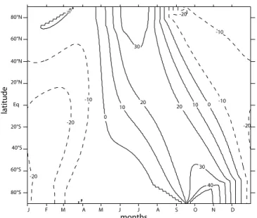
The orbital configuration for MIS4_max is relatively close to present day, with the boreal winter solstice near the peri-helion. The configuration is opposite in MIS4_min, with the boreal winter solstice occurring when the Earth is close to the aphelion (Fig. S1 in the Supplement). In the Northern Hemisphere, the precession decrease between the beginning (MIS4_max) and end (MIS4_min) of MIS4 correspond to an increase in solar radiation during boreal summer, with a max-imum in July (Fig. 1) and to a decrease during boreal winter. In the Southern Hemisphere a positive anomaly occurs dur-ing late austral winter and sprdur-ing (from July to November),

with a maximum anomaly in October south of 60◦S (Fig. 1).

-20 -20 -20 -20 -10 -10 -10 ₀ 0 0 10 10 20 20 30 30 40 va ria bl e_1 6S W dn cl ear sk y a t T OA W /m 2 19 79/ 12/ 31 0:0 :0. 0 M ea n 1 .06 89 5 M ax 56 .59 09 Mi n -41. 83 91 Eq 80 N 60 S 40 N 60 N 20 S 80 S 20 N 40 S 97 9-6 97 9-5 97 9-4 97 9-3 97 9-2 97 9-1 79 -12 79 -11 79 -10 97 9-9 97 9-8 97 9-7 J F M A M J J A S O N D -20 -20 -10 0 10 20 20 10 0 -10 30 -20 -10 30 40 80°N 60°N 40°N 20°N Eq 20°S 40°S 60°S 80°S -20 months la titude

Figure 1. Anomalies (MIS4_min-MIS4_max) in incoming solar

ra-diation at the top of the atmosphere (W m−2) averaged over the

longitude and plotted as a function of months. The figure has been plotted based on the daily insolation values.

Both simulations are run about 600 yr, until the surface cli-matic variables are at equilibrium, and we analyze averages over the last 60 yr of each simulation.

2.2 The vegetation and fire model LPJ-LMfire

2.2.1 Model description

To simulate the vegetation and fire activity in southern Africa, we use the process-based dynamic global vegeta-tion model (DGVM) LPJ-LMfire (Pfeiffer et al., 2013), a new version of the Lund-Potsdam-Jena DGVM (LPJ, Sitch et al., 2003) that includes an improved version of the SPIT-FIRE (SPread and InTensity of SPIT-FIRE) fire module (Thonicke et al., 2010). The model dynamically simulates nine differ-ent plant functional types (PFTs) (seven woody PFTs, C3 and C4 grasses), as well as the productivity and the terres-trial carbon cycle, in response to the climatic forcings,

inso-lation, atmospheric CO2level and competition between the

PFTs. The vegetation cover is described in fractions of grid cells covered by the different PFTs, which can coexist on the same grid cell. The fractional coverage of a given PFT depends on both the productivity and the individual density, which vary independently. The spatial resolution is the same

as the climatic forcings chosen by user, 0.16◦ _{in our case}

(see Sect. 2.2.2), and agricultural land use is not taken into account.

The vegetation simulated by the DGVM provides infor-mation about the fuel type and fuel load to the fire module. The fire module in turn computes fire occurrence, spread and impact on vegetation, depending on fuel information, mete-orological conditions and ignition sources. Lightning strikes

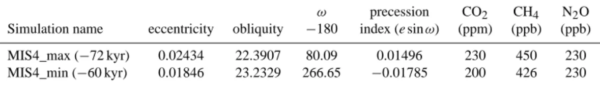
Table 1. Earth’s orbital parameters and greenhouse concentration values for the two MIS4 IPSL_CM5A simulations. ω stands for the

longitude of the perihelion and e for the eccentricity.

ω precession CO₂ CH₄ N₂O

Simulation name eccentricity obliquity −180 index (e sin ω) (ppm) (ppb) (ppb)

MIS4_max (−72 kyr) 0.02434 22.3907 80.09 0.01496 230 450 230

MIS4_min (−60 kyr) 0.01846 23.2329 266.65 −0.01785 200 426 230

are the only source of ignition taken into account in our sim-ulations.

We run LPJ-LMfire off-line, i.e., there is no vegetation feedback on climate. To drive the model we need

infor-mation on climate, soils, topography and atmospheric CO2

concentrations. The required climatic variables are monthly means of air temperature, the range of the diurnal cycle, pre-cipitation, the number of wet days, cloudiness, wind speed and lightning strike frequency, with interannual variability. A weather generator implemented in the model produces daily values from the monthly data.

2.2.2 Forcing fields

To perform vegetation and fire simulations at high resolution, we use the IPSL_CM5A outputs downscaled (see Sect. 2.3)

or interpolated to a spatial resolution of 0.16◦ as climatic

forcings. This resolution corresponds to the spatial resolution of the Climate Research Unit data (New et al., 2002) used in the downscaling method (Sect. 2.3). As mentioned previ-ously LPJ-LMfire requires forcings with interannual variabil-ity. Since the downscaling procedure provides only a mean climatology we use an anomaly procedure to build the forc-ing fields:

– We average the detrended version of a 20th century reanalysis climatology constructed by Pfeiffer et al. (2013), and increase its initial spatial resolution (0.5◦) to 0.16◦through a bilinear interpolation. We thus obtain a high-resolution mean present-day climate.

– We compute the anomaly between this mean present-day climate and the high-resolution climatology from the IPSL_CM5A simulation.

– We add the anomaly to the detrended version of the 20th century reanalysis climatology. We therefore make the assumption that there has been no change in interannual variability, which is the best approach we could follow here given the available data. It would be interesting to test this hypothesis with high-resolution regional cli-mate models in future work.

Lightning strike frequency is not simulated in IPSL_CM5A. For this variable we keep the time series constructed by Pfeiffer et al. (2013) based on a modern data set (Christian et al., 2003) and on the convective available potential energy

anomalies from the 20th century reanalysis project (Compo et al., 2011) to account for interannual variability. Similarly, soil types are taken from the standard driver data set of Pfeif-fer et al. (2013). Lightning and soil variables are simply bi-linearly interpolated to 0.16◦.

We perform three simulations of the southern African vegetation: a control simulation using the outputs of a present-day simulation of IPSL_CM5A and two MIS4 sim-ulations, using the outputs of the MIS4_max and MIS4_min

IPSL_CM5A simulations. The atmospheric CO2 level is

fixed at 310, 230 and 200 ppm (parts per million) respec-tively. For MIS4 simulations, new land points appear along the coastal edges, due to the glacial sea-level reduction. For all variables, the standard input data of Pfeiffer et al. (2013) are extrapolated on these new points using the nearest conti-nental neighbor.

Several forcing parameters change between the MIS4_min and MIS4_max LPJ-LMfire simulations: climate, insolation

and atmospheric CO2, which is known to impact vegetation

through its impact on photosynthesis and respiration rates as well as on the plant’s water-use efficiency (e.g., Jolly and Haxeltine, 1997; Cowling and Sykes, 1999; Harrison and Prentice, 2003; Prentice and Harrison, 2009; Woillez et al., 2011). To investigate the relative impact of these forc-ing factors we perform four sensitivity experiments, here-after labeled TEST_PRECIP, TEST_TEMP, TEST_CO2 and TEST_INSOL.

In TEST_PRECIP (resp. TEST_TEMP), we force LPJ-LMfire with the MIS4_max conditions, except for precipi-tation and the number of wet days (resp. the air temperature and the amplitude of the diurnal cycle) for which we take the values from MIS4_min. Thus, we isolate the impact of the change in precipitation (resp. temperature) alone when pre-cession decreases. In TEST_CO2, LPJ-LMfire is forced with

the MIS4_max climate, but with a CO2value of 200 ppm to

isolate the impact of the CO2 decrease between the

begin-ning and end of MIS4. And finally, in TEST_insol we force LPJ-LMfire with the climate of MIS4_max but impose the orbital parameters of MIS4_min: this run tests the impact of solar insolation change alone on photosynthesis and thus on vegetation productivity.

For all simulations, the model is spun up for 1080 yr, to make sure that the vegetation is at equilibrium with the cli-matic forcings. The analysis of the outputs are performed on averages over the last 60 yr of simulation.

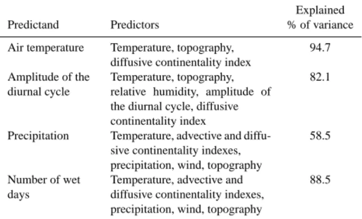
Table 2. List of the predictors selected to perform the

downscal-ing of monthly temperature and precipitation variables over south-ern Africa. The predictors “temperature”, “relative humidity”, “am-plitude of the diurnal cycle”, “precipitation” and “wind” are taken

from the IPSL_CM5A simulation and interpolated to 0.16◦. The

diffusive continentality index corresponds to the shortest distance to the ocean; the advective continentality index depends on both the wind simulated in the GCM and the distance to the ocean. See Lev-avasseur et al. (2011) for a complete description of the construction of these two predictors.

Explained

Predictand Predictors % of variance

Air temperature Temperature, topography, diffusive continentality index

94.7 Amplitude of the

diurnal cycle

Temperature, topography, relative humidity, amplitude of the diurnal cycle, diffusive continentality index

82.1

Precipitation Temperature, advective and diffu-sive continentality indexes, precipitation, wind, topography

58.5

Number of wet days

Temperature, advective and diffusive continentality indexes, precipitation, wind, topography

88.5

2.3 Statistical downscaling

To increase the spatial resolution of the AOGCM outputs re-quired to drive LPJ-LMfire at high resolution over southern Africa, we chose to apply a downscaling method and use a generalized additive model (GAM). The advantages of a GAM compared to other downscaling procedures has been shown by Wilby et al. (1998). Here we follow the approach developed by Vrac et al. (2007) for western Europe.

The downscaling procedure has been performed using the statistical programming environment R (R Development Core Team, 2009) and its "mgcv" package (Wood, 2006). The method has been developed and evaluated for the down-scaling of air temperature and precipitation (Vrac et al., 2007; Martin et al., 2011; Levavasseur et al., 2011). Here we also apply it for the downscaling of the diurnal-cycle ampli-tude and number of wet days, which by nature are expected to behave similar to temperature and precipitation respectively. The downscaling method has not been tested for cloudiness and wind speed, so these two variables were simply bilin-early interpolated to the desired 0.16◦spatial resolution.

The GAM builds statistical relationships between local-scale observations (called predictand) and large-local-scale vari-ables (called predictors, generally from fields of climate models). The expectation of the explained variable Y (the predictand) is computed by a sum of nonlinear functions, de-fined as cubic splines in our case, conditionally on the pre-dictors X (Hastie and Tibshirani, 1990):

E(Yi|Xn,n=1...k) = β0+ k X n=1 fn(Xi,n), (1) a) IPSL_CM5A Outputs bilinear interpolation statistical downscaling b) d) c) e) 8 10 12 14 16 18 20 22 24 26

mean annual temperature (°C)

-3 -2 -1 0 1 2 3 4

mean annual temperature anomaly (°C)

Figure 2. (a) Mean Annual temperature for present day simulated

by IPSL_CM5A over southern Africa (average over the years 1960– 1990 from a 20th century simulation). Mean annual temperature simulated by IPSL_CM5A for present day with a spatial

resolu-tion increased to 0.16◦through a bilinear interpolation (b) and

dif-ference with the CRU data (IPSL_CM5A – CRU) (c). Mean An-nual temperature simulated by IPSL_CM5A for present day with a

spatial resolution increased to 0.16◦through statistical downscaling

(d) and difference with the CRU data (IPSL_CM5A – CRU) (e).

where β0is the intercept, k the number of predictors and i

the grid cell.

Spline functions are piecewise third-order polynomial functions, evaluated at 4 kn. Each function has at most 12 pa-rameters. Such a model has both a great flexibility and a (rel-atively) limited number of parameters to compute (see Vrac et al., 2007 for more details).

To calibrate the GAM (i.e., to build the splines) we use the high-resolution gridded climatologies from the Cli-mate Research Unit (CRU) database (New et al., 2002) as

a) IPSL_CM5A Outputs

bilinear

interpolation statistical downscaling

b) _d)

0 200 400 600 800 1000

Annual precipitation (mm/year)

c) e)

-600 -400 -200 0 200 400 600

Annual precipitation anomaly (mm/year)

Figure 3. (a) Annual precipitation (mm yr−1) for present day simu-lated by IPSL_CM5A over southern Africa (average over the years 1960–1990 from a 20th century simulation). Annual precipitation simulated by IPSL_CM5A for present day with a spatial resolution

increased to 0.16◦through a bilinear interpolation (b) and

differ-ence with the CRU data (IPSL_CM5A – CRU) (c). Annual precipi-tation simulated by IPSL_CM5A for present day with a spatial

res-olution increased to 0.16◦through statistical downscaling (d) and

difference with the CRU data (IPSL_CM5A – CRU) (e).

predictands. For each grid-point, each data set consists of 12 monthly means (average over the period 1961–1990) at a reg-ular spatial resolution of 0.16◦in latitude and longitude, cor-responding to our downscaling resolution. To use the GAM as in Eq. (1), the distribution family of the explained variable is assumed to be Gaussian. Although temperature data classi-cally satisfy this normality assumption, precipitation values have to be log-transformed before the calibration step (Cheng and Qi, 2002).

The predictors may be divided into two groups: the “phys-ical” predictors and the “geograph“phys-ical” ones. The “physi-cal” predictors are directly extracted from a 20th century IPSL_CM5A simulation (years 1961–1990) and depend on climate dynamics. The “geographical” predictors include ge-ographical information such as topography and distance to the ocean. All the predictors must have the same spatial res-olution as the predictands. Therefore, the IPSL_CM5A out-puts used as predictors are bilinearly interpolated to 0.16◦.

The statistical relationships are established only for a given region and cannot be applied to another. Therefore, we have performed different tests to select the appropriate com-binations of predictors for southern Africa, which differ from the selection of Vrac et al. (2007) for Europe. The “optimal” predictors set is selected according to the Bayesian informa-tion criterion (BIC, Schwartz, 1978) as described by Vrac et al. (2007). The BIC allows selecting a statistical model (and the associated predictors) by balancing the risk of over-fitting.

To be evaluated in fair conditions, the GAM requires in-dependent samples between the calibration and projection steps. This condition is not satisfied for the present day since we use the same IPSL_CM5A simulation for both steps. Therefore, following Levavasseur et al. (2011), we use a “cross-validation” procedure and do the calibration on 11 months and the projection on the remaining month. With a rotation of this month we are thus able to perform the projec-tion step for any month based on an independent calibraprojec-tion data set.

To perform the downscaling for MIS4, we use the splines built for present day and project with the MIS4 predictors (for both MIS4_max and MIS4_min experiments). If the pre-dictors values for the MIS4 simulation are outside the cal-ibration range, the spline is simply linearly extrapolated to cover the whole range of the new values.

3 Results and discussion

3.1 Downscaling results for present-day southern African climate

Our best predictors’ combinations to downscale indepen-dently air temperature, diurnal-cycle amplitude, precipitation and number of wet days are listed in Table 2 with their re-spective percentage of explained variance (i.e., the percent-age of observed variance explained by a given set of explana-tory variables, Saporta, 1990):

% of variance explained = P i(y ∗ i − ¯y)2 P i(yi− ¯y)2 ×100, (2)

where y_i∗is the GAM-predicted value, yi the observed value,

and ¯ythe observed mean.

As “physical” predictors we use air temperature at the sur-face, precipitation, relative humidity, diurnal-cycle amplitude

26S 28S 30S 32S 34S

16E 20E 24E 28E 32E 16E 20E 24E 28E 32E 16E 20E 24E 28E 32E 0 0.1 0.2 0.3 0.4 0.5 0.6 0.7 0.8 0.9 1 0 0.1 0.2 0.3 0.4 0.5 0.6 0.7 0.8 0.9 1

Bare soil Trees Grasses

a) Observed modern biomes

fraction of grid-cell fraction of grid-cell

b) Observed tree cover

c) LPJ-LMfire outputs 0 0.2 0.4 0.6 0.8 1

Figure 4. (a) Modern biomes of southern Africa (Scholes, 1997; Mucina et al., 2007). (b) Observed tree cover from remote sensing data,

average over years 2001–2010 (MODIS database, Townsend et al., 2011). Grid cells with fractions < 1 % are in white. (c) Vegetation cover (bare soil, trees and grass fractions) simulated with LPJ-LMfire forced off-line by the outputs of a present-day IPSL_CM5A simulation

downscaled to 0.16◦.

and wind speed at 10 m. The “geographical” predictors are the topography and two continentality indexes. To account for the effect of local elevation on climate we use the high-resolution gridded topography ETOPO2 from the Na-tional Geophysical Data Center (NGDC, Amante and Eakins, 2008). For MIS4 we have added +70 m to this topography, to account for the reduced sea level compared to present day. The first continentality index is the “diffusive” continentality (DCO), which represents the shortest distance to the ocean (e.g., 0 % at the ocean’s edge and 100 % very remote from any ocean, corresponding to a purely continental air parcel; for southern Africa DCO reaches 100 % about 300 km from the ocean). The second continentality index is the “advec-tive” continentality (ACO). ACO is similar to DCO albeit being modulated by the large-scale wind intensities and di-rections simulated with IPSL_CM5A and represents an in-dex of the continentalization of air masses. For more details about ACO and DCO the reader is referred to Levavasseur et al. (2011).

Figures 2 and 3 illustrate the improvement of the present-day IPSL_CM5A temperature and precipitation outputs through the downscaling. When the mean annual temperature simulated with IPSL_CM5A for present day is simply

inter-polated to 0.16◦(Fig. 2b) the values are systematically lower

than the CRU data (Fig. 2c), except in the eastern mountains, where the orographic effect is not correctly captured and

the temperature is overestimated by 3–4◦C. The

downscal-ing method (Fig. 2c) corrects this cool bias and better cap-tures the temperature pattern on elevated regions (Fig. 2d). We obtain a very high percentage of variance explained for this variable (about 95 %, see Table 2). We also obtain sat-isfactory results for the amplitude of the diurnal cycle, with about 82 % of the variance explained (Table 2).

The comparison between the interpolated annual pre-cipitation simulated by IPSL_CM5A and the CRU data (Fig. 3b, c) show that the AOGCM strongly overestimates precipitation in the summer rainfall area (positive anomaly

above 600 mm yr−1) and fails to simulate the austral

win-ter precipitation in the southwest. The precipitation patwin-tern obtained after downscaling (Fig. 3d, e) reduces both biases. The percentage of variance explained is however only 58.5 % (Table 2). This relatively low percentage is in the range of the explained variance values obtained by Martin et al. (2011) for Europe. Capturing the precipitation pattern at a small spatial scale remains a challenge, given the spatially variable nature

fr

ac

tion of g

rid-cell

annual precipitation (mm/year)

bare soil

trees

grass 0 200 400 600 800 1000 1200 1400 1600

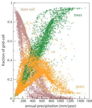
Figure 5. Vegetation cover simulated for present day with

LPJ-LMfire over southern Africa: fraction of a grid cell occupied by bare soil (brown), trees (green) and grass (yellow) vs. the total an-nual precipitation on the same grid cell.

of precipitation, thus we did not expect to reach a higher per-centage of explained variance.

The downscaling procedure assumes that the statistical re-lationships established for present-day climate are station-ary in time and remain valid for different periods. This as-sumption may be questionable in a paleoclimatic context (Vrac et al., 2007), particularly if the values of the predic-tors are outside the calibration range. In our case, most of the predictors’ values for MIS4_max and MIS4_min are still within the range of calibration, thus bringing confidence to the validity of the statistical relationships for that period. Some of the MIS4 monthly temperature values simulated by IPSL_CM5A are lower than the calibration values by a few degrees Celsius, corresponding to the austral winter temper-atures in the center of southern Africa, but the splines con-structed by the GAM for this predictor are roughly linear and a linear extrapolation should not lead to unrealistic pro-jections (see Fig. S2 in the Supplement). We are therefore confident that the method can reasonably be applied for the downscaling of the MIS4 climate over southern Africa.

3.2 Simulation of present-day vegetation and fire activity over southern Africa

3.2.1 Vegetation

The different biomes currently present in southern Africa have been initially described and classified by White (1983). This first classification has been revisited by Rutherford

(1997), Scholes (1997), and Mucina et al. (2007). Urrego et al. (2014) combine the classification of Scholes (1997) and Mucina et al. (2007) and distinguish eight different biomes: desert, Nama Karoo and Succulent Karoo (semi-desert) in the western and central regions, fynbos (Mediterranean hard-leaf scrubs) in the southern coastal regions, grasslands in the east, broad-leaved savanna in the north, fine-leaved savanna in the north and central west, and forest in the eastern coastal regions (Fig. 4a). Remote sensing data (MODIS database, Fig. 4b), (Townsend et al., 2011) show that tree fractions are above 20 % only along the coastal regions of the Indian Ocean, corresponding to the biome coastal forest and to parts of the broad-leaved savanna and fynbos. These forested re-gions appear rather fragmented, which is probably partly due to anthropogenic impacts: most tree fractions values range between 20 and 30 % and values above 50 % are limited to small patches. In regions of fine-leaved savanna, grasslands and parts of the karoo, tree fractions are below 10 %. Trees are absent in the most desertic regions in the west.

In order to evaluate the performance of LPJ-LMfire for present day, we compare qualitatively the vegetation simu-lated in the control present-day run, given as fractions of a grid cell occupied by bare soil, trees and grass (Fig. 4c) to the modern biome distribution (Fig. 4a) and to the observed tree fractions (Fig. 4b).

LPJ-LMfire simulates high bare-ground fractions in the

northwest, above 50 % west of 24◦E and north of 32◦S

(Fig. 4c), corresponding roughly to the desert and karoo re-gions (Fig. 4a). The center of the sub-continent is occupied by a mixture of bare soil, grass and trees. High grass frac-tions are simulated in the south and southwest. On the east-ern side and southeast-ern coast, including the Cape region, the model simulates forest fractions above 50 % (Fig. 4c), com-posed mainly of temperate woody PFTs.

The distribution of the simulated vegetation strongly de-pends on the annual precipitation (Fig. 5). The fraction of bare soil (trees) decreases (increases) somewhat linearly when annual precipitation increases (decreases). The grass fractions globally increase with annual precipitation between

0 and 600 mm yr−1, decrease for wetter conditions and are

replaced by trees, which are more competitive. We can dis-tinguish two peaks in the grass fractions around annual pre-cipitation values of 300 and 600 mm yr−1. The first peak cor-responds to the hinterland of the Cape region, where precip-itation occurs during the austral winter, and the second one reflects the gradual increase and decrease of grass fractions from the west to the east of southern Africa (Fig. 4a).

The presence of forests in the Cape region disagrees with observations (Fig. 4b), since the region is actually covered by the mediterranean-like scrub fynbos (Fig. 4a). This bias was expected since LPJ-LMfire does not simulate shrubs. The model also overestimates the westwards expansion of the eastern coastal forests, as well as their fractional cov-erage (> 70 %). This bias is also present when LPJ-LMfire is forced with the original data set of Pfeiffer et al. (2013),

0 0.1 0.2 0.3 0.4 0.5

fraction of grid-cell burned annually _{annual precipitation (mm/year)}

fr ac tion of g rid-cell bur ned annually

a)

b)

Figure 6. Present-day simulation of fire activity over southern Africa with LPJ-LMfire. (a) Fraction of a grid cell burned annually. (a) Annual

fraction of a grid cell burned vs. total annual precipitation on the same grid cell (mm yr−1).

based on observations and reanalyses (data not shown), and therefore can be attributed to the DGVM itself rather than to biases in the climatic forcings from IPSL_CM5A.

The overestimation of trees and underestimation of grasses compared to observations could be due either to intrinsic bi-ases of the DGVM, or to the anthropogenic influence on the modern southern African vegetation. The diverse parameter-izations used in the simulation of processes governing veg-etation dynamics or in the fire module may not be optimal for southern Africa, especially at high spatial resolution. In a similar simulation performed over Europe (data not shown) the model results show the same type of biases and over-estimates forests in the Mediterranean region, which sug-gests that the impact of a large amplitude in the hydrologi-cal seasonal cycle on vegetation is not adequately simulated in the model. The impact of fire on tree development, which has been suggested to be a determining factor in southern Africa (Westfall et al., 1983; Titshall et al., 2000; Bond et al., 2003a, b), may also be underestimated. The improvement of the model calibration may be possible, but requires further tests and comparisons with observation data at a local scale from regions without current anthropogenic impact, such as national parks.

Indeed, the model simulates the potential vegetation, i.e., without any anthropogenic disturbance such as agriculture, farming, impact on the fire regime through anthropogenic ig-nition or fire suppression, or spreading of alien plants (for more details on human impact on fire regimes in Africa, see Archibald et al. (2009, 2012). The modern landscape could be at least partly the result of human activities (Pfeiffer et al., 2013). This hypothesis is supported by pollen data from the

marine core MD96-2048, off the coast of eastern southern Africa (Dupont, 2011), which show higher percentages of tree pollen during the last interglacial, when human impact was likely negligible.

3.2.2 Fire

For present day, LPJ-LMfire simulates fires mainly in the

center of southern Africa, between 23 and 27◦E, and in the

south, between 31–33◦S. In these two regions, annual burned

area fractions are around 20–30 and 30–40 % respectively (Fig. 6a). In other words, fires occur outside the desert re-gion on the western side, where fuel load is too small to sus-tain fires, and outside of the regions where humidity and tree fractions are high (Fig. 4c).

Figure 6b shows the annual fraction of a burned grid cell plotted against annual precipitation. The model simulates

two peaks in fire activity, around 300 and 600 mm yr−1,

cor-responding to the grid cells with the maximum fractions of

grass (Fig. 5b). For precipitation above 600 mm yr−1, the

burned fractions steeply decrease, reflecting the lower fire activity for wetter conditions and high tree fractions. Below

300 mm yr−1_{, fire activity also decreases, following the}

de-crease in available fuel load.

The maximum burned area fractions simulated with LPJ-LMfire are about three to four times higher than modern ob-servations of fire activity in southern Africa: for the period 1997–2011, the average annual burned area fractions are be-low 5 % (Giglio et al. (2010); http://globalfiredata.org; data for southern Africa shown on Fig. S3 in the Supplement).

-5 -4 -3 -2 -1 0 1 2 3 4 5 -3 -2.5 -2 -1.5 -1 -0.5 0 0.5 1 1.5 2 2.5

°C mm/day

Temperature Precipitation

b) MIS4_min - MIS4max DJF a) MIS4_min - MIS4_max JJA

Temperature Precipitation

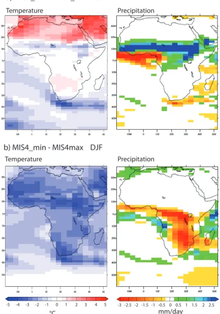
Figure 7. Difference in mean temperature (◦C) and mean precipitation (mm day−1) simulated with IPSL_CM5A between the beginning and end of MIS4 (MIS4_min–MIS4_max). (a) Average for the boreal summer months (June–August); (b) average for the boreal winter months (December–February).

Our results are in agreement with Pfeiffer et al. (2013), i.e., without agricultural land cover. If agriculture is taken into account and lightning-caused fires are excluded from the cultivated areas, results are in good agreement with observa-tions (Pfeiffer et al., 2013), which suggests a strong influ-ence of human activity through agriculture on the modern fire regime of southern Africa. The overestimation of an-nual burned fractions in southern Africa in our simulations can thus be attributed to the absence of agricultural land use and does not prevent the analysis of the response of the fire regime to paleoclimatic changes.

3.3 Climate, vegetation and fire response to precession changes for MIS4 conditions

3.3.1 Climate

Here we focus on the temperature and precipitation changes when precession decreases for MIS4 boundary conditions (MIS4_min–MIS4_max) over Africa. The mean features of the temperature and precipitation anomalies at global scale simulated in MIS4_max compared to present day can be found in the Supplement (Fig. S4 in the Supplement). Here we focus on the temperature and precipitation changes when precession decreases for MIS4 boundary conditions (MIS4_min–MIS4_max) over Africa.

16E 18E 20E 22E 24E 26E 28E 30E 32E 34E -300 -250 -200 -150 -100 -50 0 50 100 150 annual precipitation anomaly (mm/year) 26S 27S 28S 29S 30S 31S 32S 33S 34S 35S 26S 27S 28S 29S 30S 31S 32S 33S 34S 35S _{a) MIS4_max - Present} b) MIS4_min - MIS4_max

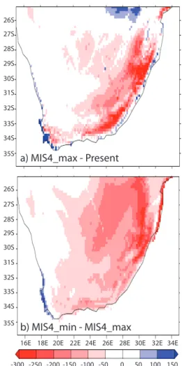
Figure 8. Annual precipitation (mm yr−1) simulated by

IPSL_CM5A and downscaled to 0.16◦for (a) MIS4_max–present,

and (b) MIS4_min–MIS4_max.

The increase in boreal summer insolation (JJA) in the Northern Hemisphere (Fig. 1) leads to higher temperatures over Africa north of 30◦N (Fig. 7a) and to the intensification of the northern African monsoon in response to the enhance-ment of the land–sea temperature contrast. Precipitation over the Sahel is intensified and shifted northward, due to the

en-hancement of the monsoon winds. Precipitation around 4◦N

decreases as moisture is advected more inland, whereas we

observe a positive precipitation anomaly around 10◦N. The

negative anomaly in temperature in the same latitude band is caused by the increase in the latent heat flux associated to the wetter conditions. The mechanism described here is qualita-tively similar to the simulation results of Marzin and Bracon-not (2009b) for the Holocene. We leave the detailed investi-gation of the differences in the northern African monsoon sensitivity to precession for the Holocene or MIS4 bound-ary conditions for another study. We simply point out here the persistence of the mechanism for the MIS4 glacial condi-tions.

During the austral summer (DJF) the negative insolation anomaly over both hemispheres in MIS4_min compared to MIS4_max (Fig. 1) leads to a global cooling over Africa

(Fig. 7b), ranging from −1 to −4◦C, depending on the

re-gion considered. For precipitation, the model simulates drier

conditions south of 5◦N, over the regions under the

influ-ence of the ITCZ during DJF. This drying can be linked to the lower temperatures, causing a decrease in the intensity of the convection. Thus, our results show an opposite response of the northern African monsoon and the southern African monsoon to precession changes, at least for the MIS4 glacial boundary conditions.

After downscaling, the climate simulated in southern Africa in the summer rainfall region (eastern part) for MIS4_max is drier than the modern one, with total annual

rainfall anomalies between −50 and −300 mm yr−1

(Fig. 8a). The decrease of precession (MIS4_min–

MIS4_max) leads to an additional drying in the east

(from −100 to −200 mm yr−1over most part of the summer

rainfall area) and in the center (from −50 to −100 mm yr−1

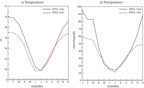
around 22◦E) (Fig. 8b). Figure 9 presents the annual cycle of

the downscaled temperature and precipitation over the area of summer rainfall (DJF) for MIS4_max and MIS4_min. The precession decrease leads to a decrease of the amplitude of the seasonal cycle of both temperature and precipitation. The austral summer (DJF) is drier and cooler, with a maxi-mum precipitation decrease in December and January of 40

and 35 mm month−1 respectively, i.e., a decrease of 37 and

46 %. The drying is accompanied by a 3◦C cooling in the

monthly temperature. No significant changes in precipitation or temperatures occur during the winter months (JJA).

Our results confirm a strong impact of precession on the hydrological cycle of the region. The simulations results are in qualitative agreement with the data from the Pretorian Saltpan, in the north of southern Africa (Partridge et al., 1997; Kristen et al., 2007). The analysis of the lacustrine sediments from this site, covering the last 200 000 yr, show periodic variations between wet and dry periods at the pre-cessional frequency (23 ky). However, absolute dating, based on radio-carbon analysis, only covers the first 43 ky of the sequence, preventing the determination of a precise phasing relationship between rainfall and precession changes. Kris-ten et al. (2007) have suggested that precipitation changes at the Pretorian Saltpan could be related to changes in the intensity and/or the length of the rainy season in that re-gion. Our IPSL_CM5A simulations does not show changes in the length of the rainy season when precession decreases, but rather a flattening of the hydrological cycle with less intense rainfall from November to March. Partridge et al. (1997) have estimated the sensitivity of the southern African summer rainfall to insolation changes to 4.5 (i.e., 1 % crease in summer insolation produces 4.5 % precipitation in-crease). The annual downscaled precipitation in the region of the Pretorian Saltpan in MIS4_min and MIS4_max are 615

months months °C mm/mon th a) Temperature b) Precipitation MIS4_max

MIS4_min MIS4_maxMIS4_min

J F M A M J J A S O N D J F M A M J J A S O N D

Figure 9. Annual cycle of (a) mean monthly temperatures (◦C) and (b) mean monthly precipitation (mm month−1) over the east of southern

Africa (summer rainfall area, 37–25◦S, 22–35◦E simulated in MIS4_max (black) and MIS4_min (red) (IPSL_CM5A simulations,

down-scaled to 0.16◦)).

insolation at 30◦S of 463 and 495 W m−2, i.e., a 25 %

pre-cipitation increase for 7 % insolation increase. The precipita-tion sensitivity coefficient computed from these values is thus 3.5, smaller than the results of Partridge et al. (1997) but of the same order of magnitude. However, even when the record from the Pretorian Saltpan is tuned on the precession varia-tions, the reconstructed precipitation at the Pretorian Saltpan

and insolation at 30◦S diverge after 60 kyr. Our simulations

thus correspond to the very last period where precession and summer rainfall in southern Africa seem to co-vary. How-ever, since we performed only snapshot simulations, we can-not investigate the possible leads and lags between preces-sion and precipitation changes to validate or invalidate the tuning of Partridge et al. (1997). AOGCMs are not suitable tools to investigate this issue, given their high computational cost. Simulations with faster AOGCMs would be required to perform transient runs and to investigate further the links be-tween precession and precipitation in southern Africa over several precession cycles.

3.3.2 Vegetation changes in southern Africa

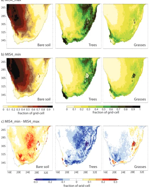
The vegetation pattern simulated over southern Africa for MIS4_max (Fig. 10a) is close to the one simulated for present day (Fig. 4b), with high tree fractions in the east. The high tree percentages in that region seem to be more in a qualitative agreement with pollen data for MIS4 than for present day. Indeed, pollen data from marine core MD96-2048 (off the eastern southern African coast; Dupont, 2011) show about 40 % of tree pollen at the beginning of MIS4 vs. about 20 % for present day. This observation suggests that part of the present day mismatches between the vegetation

model and actual observations might indeed be attributed to anthropogenic effects (Sect. 3.2.1).

In MIS4_min (Fig. 10b, c) bare soil fractions increase southwards and eastwards at the expense of grasses and trees.

In the center of southern Africa (22◦_–28◦_{E) the model}

sim-ulates increases in the bare soil fractions between 10 and 25 %. An increase of similar magnitude also occurs in the southwest. Decreases in tree fractions (between 5 and 25 %) occur on all grid cells where they are present in MIS4_max (Fig. 10c). The total decrease in the area occupied by trees over southern Africa is between about 18–19 % for the ev-ergreen woody PFTs and 30 % for the summev-ergreen trees (Fig. 11a). Grass fractions decrease by 5–15 % in the cen-ter and southwest but increase in the east and south at the expense of trees (Fig. 10c). Overall, the total area covered by grasses over southern Africa decreases by about 7 % (Fig. 11a).

The simulated increase in the bare soil fractions can be considered as a desertification of the landscape and is in qualitative agreement with pollen data off western southern Africa (marine core MD96-2098), which show an expansion in the semi-desert biomes (Urrego et al., 2014) when pre-cession decreases during MIS4. Likewise, our results are in agreement with the increase in arboreal pollen off eastern southern Africa during the same period (marine core MD96-2048, Dupont, 2011).

The results of the sensitivity runs are synthesized in Fig. 11a, which shows the percentages of change in the total area occupied by the different PFTs for each simulation com-pared to MIS4_max. The diagrams show that relative impact of the different factors that we tested (precipitation,

a) MIS4_max

b) MIS4_min

c) MIS4_min - MIS4_max Bare soil

Bare soil

Bare soil Trees Trees Trees Grasses Grasses Grasses 0 0.1 0.2 0.3 0.4 0.5 0.6 0.7 0.8 0.9 1 0 0.1 0.2 0.3 0.4 0.5 0.6 0.7 0.8 0.9 1 26S 28S 30S 32S 34S 26S 28S 30S 32S 34S 26S 28S 30S 32S 34S

16E 20E 24E 28E 32E 16E 20E 24E 28E 32E 16E 20E 24E 28E 32E

fraction of grid-cell fraction of grid-cell

-0.3 -0.2 -0.1 0 0.1 0.2 0.3 fraction of grid-cell

Figure 10. Vegetation cover (fraction of grid cell) simulated with LPJ-LMfire forced off-line. (a) MIS4_max, (b) MIS4_min, and (c)

MIS4_min–MIS4_max.

– Trees: the CO2 decrease between MIS4_max and TEST_CO2 is only 30 ppm, but is responsible for a decrease between 3 and 7 % for the three woody PFTs. This result is not very surprising given that LPJ

is a DGVM rather sensitive to CO2 concentrations

(e.g., Köhler et al., 2005). Temperature changes alone (TEST_TEMP) lead to an increase of the temperate needleleaf evergreen trees and the temperate broadleaf evergreen trees of +11 and +4.5 % respectively but to a small decrease of the temperate broadleaf sum-mergreen trees (−5 %). Changes caused by insolation changes (TEST_INSOL) are smaller than 3 % for the three temperate woody PFTs. The changes simulated in

TEST_PRECIP are close to the changes obtained for MIS4_min compared to MIS4_max.

– Grasses: the changes in the total area occupied by grasses for MIS4_min compared to MIS4_max is about

−7 %. The changes simulated in the different sensitivity

runs compared to MIS4_max are small, with less than 1 % of variations in TEST_PRECIP and TEST_TEMP and about −3 % in TEST_CO2 and TEST_INSOL. Precipitation changes alone are sufficient to simulate a de-crease in the surfaces occupied by the woody PFTs, sim-ilar to the decrease obtained for MIS4_min. Precipitation changes thus appear as the main factor driving the changes in tree fractions when precession decreases (MIS4_min–

-35 -30 -25 -20 -15 -10 -5 0 5 10 15 MIS4f MIS4d2 + precip MIS4f MIS4d2+tempMIS4f MIS4d2+co2 MIS4f MIS4d2 + insol MIS4f 15 10 5 0 -5 -10 -15 -25 -30

TempBE TempBS Grass

-20 -25 -20 -15 -10 -5 0 5 10 15 20 MIS4f-MIS4d2% PRECIP% 0 5 10 15 -5 -10 -15 -20 East Center Total g rass sur fac e anomalies (%) Sur fac e anomalies (%) MIS4_min - MIS4_max TEST_PRECIP - MIS4_max TEST_TEMP - MIS4_max TEST_CO2 - MIS4_max TEST_INSOL - MIS4_max MIS4_min - MIS4_max TEST_PRECIP - MIS4_max TEST_TEMP - MIS4_max TEST_CO2 - MIS4_max TEST_INSOL - MIS4_max b) TempNE a)

Figure 11. Percentage of changes in (a) the total surface

oc-cupied by temperate needleleaved trees (TempNE), temperate broadleaved evergreen trees (TempBE), temperate broadleaved summergreen trees (TempBS) and grasses; (b) the total surface

occupied by grasses in the east (34–25◦S, 27–34◦E) and in the

center (33–25◦S, 19–27◦E) of southern Africa, in MIS4_min,

TEST_PRECIP, TEST_TEMP, TEST_CO2 and TEST_INSOL compared to MIS4_max.

MIS4_max). The relative impact of temperature, insolation

and CO2changes between MIS4_min and MIS4_max

com-pensate each other. The sensitivity of grasses at the scale of southern Africa as a whole to the different factors tested is less clear. In particular, contrary to the woody PFTs, grasses seem to be insensitive to precipitation changes. However, this result hides important spatial differences between the east, where grasses increase with precession decrease and the cen-tral areas, where grass fractions decrease (Fig. 10). In the eastern part, precipitation decrease is the main driver of the expansion of grasses (Fig. 11b). In the center, the total de-crease in grass surface is about −22 %. Precipitation changes

alone lead to a decrease of −10 % and the CO2decrease to a

decrease of −7 %. These differences in the response of grass between the east and the center of southern Africa can be ex-plained by the vegetation dynamics and the competition with the woody PFTs. In the east, the precipitation decrease drives the regression of trees but grasses have smaller water require-ments and can expand on the space left by the woody PFTs. In the center, where annual precipitation is lower, the drying of climate affects both grasses and trees and the first driver of the regression of grasses is the precipitation decrease.

How-26S 27S 28S 29S 30S 31S 32S 33S 34S 16E 35S

20E 24E 28E 32E

-0.3 -0.2 -0.1 0 0.1 0.2 0.3 Fraction of grid-cell burned annually

MIS4_min - MIS4_max

Figure 12. Difference (MIS4_min–MIS4_max) in the percentages

of a grid cell burned during a year when precession decreases.

ever, the impact of the CO2decrease is of similar magnitude

and appears as an important factor to explain grass changes.

3.3.3 Fire activity changes in southern Africa

Figure 12 shows changes in the percentages of a grid cell burned annually when precession decreases (MIS4_min– MIS4_max). The LPJ-LMfire model simulates a decrease in fire activity in the center of southern Africa (from −5 to

−20 %) and an increase in the east and south (from +5 to

+10 %). The comparison between Figs. 12 and 10 shows that fire activity increases when grass fractions increase and de-creases where grass and/or tree fractions decrease. As men-tioned in the previous section, the grass increase in the east and south merely reflects the regression of trees and is there-fore strongly dependent on the vegetation’s initial state in MIS4_max.

To better visualize this relationship between vegetation changes and fire activity we have plotted the changes in bare soil, tree and grass fractions against changes in the annual burned surface on Fig. 13a. The graph clearly shows a de-crease in burned fractions over grid cells where bare soil fractions increase and tree and grass fractions decrease, and an increase in burned fractions with higher grass fractions (Fig. 13a). On the contrary, no clear relationship appears be-tween the amplitude of the annual precipitation changes and the fire activity (Fig. 13b). This can be attributed to a differ-ent vegetation response in the east and in the cdiffer-enter of south-ern Africa. In the east, despite the precipitation decrease, the climate is still wet enough to allow an increase of grass (i.e., easily incinerable fuels), whereas in the center the climate

Fraction of grid-cell burned annually anomalies Fraction of grid-cell burned annually anomalies Vegeta tion fr ac tions anomalies A nnual pr ecipita

tion anomalies (mm/y

ear)

a) b)

bare soil trees

grass

Figure 13. (a) Anomalies in the fraction of a grid cell occupied by bare soil (brown), trees (green), grasses (yellow) vs. anomalies in the

percentage of a grid cell burned annually (MIS4_min–MIS4_max). (b) Total annual precipitation anomalies (mm yr−1) vs. anomalies in the

percentage of a grid cell burned annually (MIS4_min–MIS4_max).

has become too dry and grasses decline, leading to smaller amounts of light fuel and a decrease of fire.

At the scale of the whole southern Africa, the dominant signal is the regression of grass-fueled fires in response to the precipitation decrease in the summer rainfall area, in qualitative agreement with Daniau et al. (2013). The simu-lations confirm the link between precession and fire activ-ity, inferred from the microcharcoal record. As discussed in Daniau et al. (2013), the record can reflect either shifts in grassland extent or shifts in grassland productivity. Daniau et al. (2013) conclude that the latter hypothesis was the most likely. Our modeling results support this conclusion. Indeed, LPJ-LMfire simulates changes in vegetation fractions mainly limited to 5–15 % for trees and 5–10 % for grasses (Fig. 10c) in most parts of southern Africa. Such percentages reflect changes in the productivity and density of the PFTs, but are not large enough to be interpreted as biome shifts.

Our results suggest that precession decrease appears to im-pact fire activity mainly indirectly, via changes in fuel load, rather than directly via changes in humidity. It confirms that vegetation response to climate changes have to be taken into account to investigate fire changes and highlight the impor-tance of fuel load and how increased dryness can paradoxi-cally lead to a decrease in fire activity in southern Africa.

Such a conclusion has been previously suggested for the last 21 kyr (Turner et al., 2008) and during the last glacial period (Daniau et al., 2007) in the Mediterranean region.

4 Conclusions

We have performed two simulations of the MIS4 climate with the AOGCM IPSL_CM5A, for a maximum and mini-mum of the climatic precession index, and analyzed the sim-ulated climatic changes over Africa, with a focus on south-ern Africa. The decrease of the precession index leads to an increase of boreal summer insolation in the Northern Hemisphere and to an intensification of the northern African monsoon. On the contrary, insolation decrease during aus-tral summer leads to a cooling over Africa and to a decrease in the convective activity associated to the ITCZ, leading to a decrease of precipitation over the regions under its influ-ence, including the east of southern Africa. Thus, our results show an anticorrelation between the northern and southern African monsoons in response to precession changes for the MIS4 glacial boundary conditions.

The IPSL_CM5A outputs have been statistically down-scaled or interpolated to obtain high-resolution fields. These fields are used as input for the dynamic vegetation model LPJ-LMfire, to simulate vegetation and fire changes over southern Africa in response to precession changes.

The simulated potential present-day vegetation presents some biases compared to observations, but the model–data discrepancies are probably mostly due to the anthropogenic impact on the modern southern African vegetation. For our MIS4 vegetation simulations we can achieve the follow-ing conclusions, in qualitative agreement with observations: (i) precession decrease leads to a decrease of precipita-tion during austral summer in eastern southern Africa (sum-mer rainfall area). No significant precipitation changes occur during the dry season. (ii) The dryness increase causes an

expansion of bare soil, which can be interpreted as a deser-tification, and a decrease in trees and grass fractions in the center of southern Africa. In the east, the model simulates an expansion of grasses in response to the precession decrease, due to their development on grid cells where tree cover de-clines. (iii) The simulated fire activity over southern Africa is strongly dependent on the vegetation type (i.e., fuel load) and decreases (increases) on grid cells where grass fractions decrease (increase).

The results provided here show important climatic and environmental changes in southern Africa between the be-ginning and end of MIS4. How they could have affected the early human populations in that region could be tack-led through ecological niche modeling (Banks et al., 2008). However, our simulations do not take into account the impact of millennial-scale variability, which is superimposed to the long-term orbitally driven climatic changes and was recently suggested as a driver of technological innovations (Ziegler et al., 2013). This issue requires supplementary runs with the IPSL_CM5A model, similar to the freshwater-hosing experi-ments that have been performed with the older version of the GCM and for last glacial maximum conditions (Kageyama et al., 2009; Woillez et al., 2013).

The Supplement related to this article is available online at doi:10.5194/cp-10-1165-2014-supplement.

Acknowledgements. The present manuscript is a contribution to

the TRACSYMBOLS project, supported by the European research council, TRACSYMBOLS no. 249587. This work also benefited from the HPC resources of CCRT and IDRIS made available by GENCI (Grand Equipement National de Calcul Intensif), CEA (Commissariat a l’Energie Atomique et aux Energies Alternatives) and CNRS (Centre National de la Recherche Scientifique). We thank Olivier Marti for his help in the construction of the correct boundary conditions for the GCM, Jed Kaplan for providing the LPJ-LMfire model and Stefan Kern for providing MODIS files. We also thank two anonymous reviewers for their comments to improve this manuscript.

Edited by: V. Brovkin

The publication of this article is financed by CNRS-INSU.

References

Amante, C. and Eakins, B.: Etopo1–1 arc-minute global relief model: procdures, data sources and analysis, Technical report,

National Geophysical Data Center, NESDIS, NOAA, US Depart-ment of Commerce, National Geophysical Data Center, Boulder, Colorado, 2008.

Archibald, S., David, R., Van Wilgen, B., and Scholes, R.: What limits fire? an examination of drivers of burnt area in southern africa, Global Change Biol., 15, 613–630, 2009.

Archibald, S., Scholes, R., Roy, D., Roberts, G., and Boschetti, L.: Southern African fire regimes as reaveled by remote sensing, J. Wildland Fire, 19, 861–878, 2010.

Archibald, S., Staver, A., and Levin, S.: Evolution of human-driven fire regimes in africa, Proc. Natl. Acad. Sci., 109, 847–852, 2012. Argus, D. and Peltier, W.: Constraining models of postglacial re-bound using space geodesy: a detailed assessment of model ICE-5G (VM2) and its relatives, Geophys. J. Int., 181, 697–723, 2010. Banks, W., d’Errico, F., Townsend Peterson, A., Vanhaeren, M., Kageyama, M., Sepulchre, P., Ramstein, G., Jost, A., and Lunt, D.: Human ecological niches and ranges during the LGM in Eu-rope derived from an application of eco-cultural niche modeling, J. Archeol. Sci., 35, 481–491, 2008.

Bond, W., Midgley, G., and Woodward, F.: The importance of low

atmospheric CO2and fire in promoting the spread of grasslands

and savannas, Global Change Biol., 9, 973–982, 2003a. Bond, W., Midgley, G., and Woodward, F.: What controls South

African vegetation – climate or fire ?, South Afr. J. Botany, 69, 79–91, 2003b.

Braconnot, P. and Marti, O.: Impact of precession on monsoon char-acteristics from coupled ocean atmosphere experiments: changes in Indian monsoon and Indian ocean climatology, Mar. Geol., 1– 3, 23–24, 2003.

Braconnot, P., Joussaume, S. de Noblet, N., and Ramstein, G.: Mid-Holocene and last glacial maximum African monsoon changes as simulated within the Paleoclimate modelling intercomparison project, Global Planet. Changes, 26, 51–66, 2000.

Cheng, M. and Qi, Y.: Frontal Rainfall-Rate Distribution and some conclusions on the threshold method, J. Appl. Meteorol., 41, 1128–1139, 2002.

Christian, H., Blakeslee, R., Boccippio, D., Boeck, W., Buechler, D., Driscoll, K., Goodman, S., Hall, J., Koshak, W., Mach, D., and Stewart, M.: Global frequency and distribution of lightning as observed from space by the optical transient detector, J. Geo-phys. Res.-Atmos. (1984–2012), 108, ACL4-1–ACL4-15, 2003. Compo, G., Whitaker, J., Sardeshmukh, P., Matsui, N., Allan, R., Yin, X., Gleason, B., Vose, R., Rutledge, G., Bessemoulin, P., Brönnimann, S., Brunet, M., Crouthamel, R., Grant, A., Grois-man, P., Jones, P., Kruk, M., Kruger, A., Marshall, G., Maugeri, M., Mok, H., Nordli, E., Ross, T., Trigo, R., Wang, X., Woodruff, S., and Worley, S.: The Twentieth Century Reanalysis Project, Q. J. Roy. Meteorol. Soc., 137 1–28, 2011.

Cowling, R., Richardson, D., and Pierce, S. (Eds.): Vegetation of Southern Africa, Cambridge University Press, 1997.

: (1999). Physiological significance of low atmospheric CO₂for

plant-climate interactions, Quaternary Res., 52, 237–242, 1999. Daniau, A.-L., Sanchez-Goñi, M.-F., Beaufort, L.,

Laggoun-Défarge, F., Loutre, M.-F., and Duprat, J.: Dansgaard-Oeschger climatic variability revealed by fire emissions in southwestern Iberia, Quaternary Sci. Rev., 26, 1369–1383, 2007.

Daniau, A.-L., Sánchez-Go˜i, M.-F., Martinez, P., Urrego, D., Bout-Roumazeilles, V., Desprat, S., and Marlon, J. R.: Orbital-scale