Synchronization in Music Group Playing

(1)

HAL Id: hal-01257540

https://hal.archives-ouvertes.fr/hal-01257540

Submitted on 17 Jan 2016

HAL is a multi-disciplinary open access

archive for the deposit and dissemination of

sci-L’archive ouverte pluridisciplinaire HAL, est

destinée au dépôt et à la diffusion de documents

Iris Yuping Ren, René Doursat, Jean-Louis Giavitto

To cite this version:

Iris Yuping Ren, René Doursat, Jean-Louis Giavitto. Synchronization in Music Group Playing.

Inter-national Symposium on Computer Music Multidisciplinary Research (CMMR), Jun 2015, Plymouth,

United Kingdom. 510–517 (in electronic proceedings). �hal-01257540�

(2)

3 _{Institut de Recherche et Coordination Acoustique/Musique (IRCAM),}

CNRS (UMR9912), Paris, France yuping.ren.iris@gmail.com

Abstract. In this project, we created an agent-based model of music group playing under four di↵erent interaction mechanisms. Based on real music data, added randomness and simplifying assumptions, we examine how agents synchronize and deviate from the original score. We find that while music can make synchronization complex, it also helps reducing the total deviation. By studying the simulation process, several conclusions on the relationship between di↵erent growing speeds of total deviations and di↵erent interaction schemes are drawn. With interpretation from a musical point of view, we find that, in a music ensemble, listening to neighbors helps the players end up in sync. However, if people do not listen carefully enough, the deviation becomes larger than when people do not listen at all. On the issue of whom one should listen to, the results show no significant di↵erences between listening to the immediate neighbors and to the whole group. Finally, we also observe that large deviations can be reduced by making the musicians move while playing. Keywords: synchronization, collective behavior, agent-based modeling, deviation, music playing

1 Introduction

Many questions have been asked about the rhythmic complexity of music. Is it more difficult to synchronize over a melodic rhythm or a drum beat? Is it better to listen to people around you or just play as written in a music ensemble? How can we obtain better synchronization? Several research papers and books have addressed synchronization problems in biological and social/human interaction systems [1–5], but few have answered this line of questions. In this project, we simulate music ensembles using agent-based models, a method known for its abil-ity to produce complex behaviors from simple rules. Although it is not possible for simple models to accurately represent every interaction among musicians, it is still possible to gain valuable insights from abstractly simulated music ensem-bles.

Two important concepts embedded in this project are derived from the well-known “firefly” model of synchronization [5]. Like this model, we define phase

(3)

2 Iris Yuping Ren, Ren´e Doursat, and Jean-Louis Giavitto

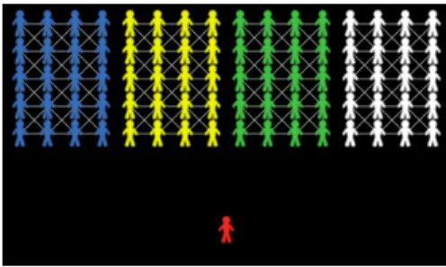
Fig. 1. Initial configuration of the music group program, with a conductor symbolized in red and four di↵erent groups of musicians in “white”, “green”, “yellow”, and “blue”.

and frequency variables to characterize the system. Herre, the frequency of each agent will be called “tempo” and the phase lag, the “the waiting time”. Im-portant di↵erences with the firefly model are the incorporation of actual music data and conditional interactions between musicians. Another important con-cept is the unavoidable deviation of the played stream from the written music, which has been investigated in [6–8] and experimentally proven. Although we do not have such a small time resolution, the implementation can be justified with amateur music players.

2 Model

In this model, we use real music data in the form of duration datasets (without pitch), extracted from Beethoven’s quartets. The players follow these durations and di↵erent interaction schemes among themselves. We simulate music ensem-bles consisting of four sections, “white”, “green”, “yellow”, and “blue” (Fig. 1), so that we can observe the di↵erences between schemes applied inside each sec-tion. Musical interactions between two sections are ignored for simplicity. Some amount of spatial interaction between players will be introduced at a later stage. 2.1 Parameters

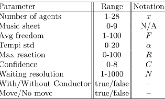
The parameters of the model are the following (Table 1):

– Number of agents: how many agents there are in one musical section. – Music sheet: 10 di↵erent music datasets (rhythmic parts only, no pitch);

1-8 are the Beethoven string quartets Nr. 1-1-8; 0 and 9 are drum beats with intervals of 1 and 3 seconds.

– Avg freedom: mean of the freedom of agents (with default standard devia-tion, modifiable from the program itself).

– Tempi std: standard deviation of the tempi of agents (with default mean value, modifiable from the program itself).

(4)

Move/No move true/false –

Table 1. Table of model parameters with the range of acceptable values and mathe-matical notations

– Max reaction: maximum value of the reaction skills of agents (where actual skill is a random integer number under this cap, modifiable from the program itself).

– Confidence: how many actively playing neighbors one musician must have, in order to be confident that s/he is playing at the right time.

– Waiting resolution: a normalizing factor controlling in part how much time resolution a musician has.

– With/without conductor: this is just for the yellow group; the tempo will be set uniformly to 100 if this is on and the players became aware that they are playing “wrongly”.

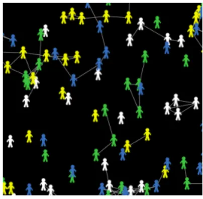
– Move/no move: agents will move randomly if this is on, as shown in Fig. 2. Their neighbors will therefore also change.

To have a concrete view of the e↵ect of these parameters, we explain the dy-namics of the model in the next section.

2.2 Dynamics

The mechanism used to synchronize the musicians is based on the music. For every note duration in the dataset, we approach it using a timer, which is reset at the beginning of every step. The value of the timer is denoted by t(i), where i is the step number in the process, which is equal to the number of duration values in the dataset. Then, once the timer’s value and the note’s duration m(i) are sufficiently close, we ask the agents, which are by default in color gray, to change to the color belonging to their group (white, green, yellow, blue), hence achieve an e↵ect of “playing” the event. We will also use the word “recoloring” to denote music playing. We denote each agent by x, as mentioned in the parameter table. For describing the relation between a parameter and the turtles-owned value controlled by it, we use a functional notation. For example, each turtle’s reaction skill will be denoted by R(x). Considering all the parameters we used above, this part of the dynamics can be expressed as:

if m(i) ↵(x)

100 ⇥ t(i) > F (x)

(5)

Fig. 2. Typical motion dynamics.

otherwise, recolor. The next time the agent becomes gray can happen at the next step, when the timer discovers that there is still a certain amount of time until the end of the next duration.

Finally, we add interactions among players to the process, asking agents to “look” whether there are enough players around them who are playing. If that number is larger than the confidence level of a player, C, then s/he must change the tempo according to the mean of the active neighbors, denoted by_{xk}k2[0,28]

(explained in detail in the next paragraph). We denote the number of the gray linked-neighbors by nx, and write this part of the dynamics:

if nx C, tempo(x) := tempo(xk)

After all this decision making, we record the actual di↵erence between the waiting time and the duration, and plot this deviation. Di↵erences between the four group reside in how they react to other players’ tempi, i.e. the di↵erences between the_{xk}:

– Players in the white group listen to other neighboring white players and take the mean tempo from them.

– Players in the green group listen to other neighboring green players, but follow a normal distribution whose mean is equal to the average tempo of the neighbors.

– Players in the yellow group have two choices: when the conductor option is on, they sync to the conductor, i.e. adopt a uniform tempo; otherwise, they listen to all other players in all groups.

– Players in the blue group listen to all other blue players and take the mean tempo from them.

We also introduce a motion dynamics, while the “Move” option is on, we ask the players to move randomly, including changes in their links; that is, their neighbor will change according to where they are.

(6)

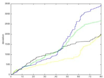
(a) Time series of the total deviations of the white (shown in black), green, yellow and blue groups, featuring the large deviation of the green group. Other groups have similar lower total devia-tions. The “conductor switch” for the yellow group is on. Other di↵erent grow-ing patterns between the white, yellow and blue groups are caused by the speci-ficties of the music at hand.

(b) Time series of the total deviations of the four groups when musicians are mov-ing. Here, the blue group is strongly in-fluenced by the bad tempi of the green players. In other runs, the group that gets most influenced might change. In general, however, there is no outlier curve of total deviation like the green one in (a).

Fig. 3. Time series of total deviations: (a) static players; (b) moving players.

2.3 Statistics

The following statistics are used to measure the outcome of our model:

– Each group’s total deviation from the music, called “total deviation 1”, etc. – Each player’s deviation from the music (because the total deviation loses the

information about whether individual players are lagging or leading). – The tempo distribution of the players over each group; synchronization

among players can be observed when these distributions converge.

– The deviation distribution of the players; most are centered around zero, oth-ers account for the cumulative deviation that we show in the total deviation window.

3 Results

In the beginning of the simulation, tempi are scattered in all four groups, and total deviations grow with time in a similar manner. We can also see the conver-gence of tempi in certain groups. After observing the process for a while, we find di↵erent growing speeds of the total deviation between di↵erent groups. The green group exhibits a particularly big deviation as shown in Fig. 3(a). After running for a period of time, the program slows down. This should not matter

(7)

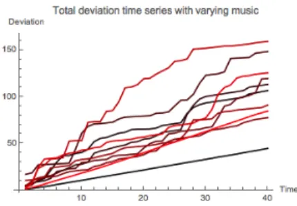
(a) Time series of the total deviations of the white group for di↵erent music pieces. Real music is adding complex-ity to the drum-beat music. Listening to neighbors results in larger deviation than the group with the conductor for drum-beat music, but smaller deviation for real music.

(b) Time series of the total deviations of the green group for di↵erent music pieces. Compared to the Beethoven mu-sic, the drum-beat music leads to fast growth in deviation. The complexity of music prevents the generation of devi-ation upon devidevi-ation. The curve with larger curvature is the drum beat of 3-second intervals.

(c) Time series of the total deviations of the yellow group for di↵erent music pieces. Real music is adding complex-ity to the drum-beat music. With the conductor, the drum-beat music has the least deviation. The linear growth rates are close, also resulting from having a conductor in lead.

(d) Time series of the total deviations of the blue group for di↵erent music pieces. The linear growth of the drum-beat mu-sic is at around the same level of the Beethoven music. The linear growth with larger slope is the drum beat of 3-second intervals.

Fig. 4. Total deviation time series of all four groups with di↵erent music pieces

much for the project because when deviations become large, the ensemble usu-ally stops playing. However, there are cases when musicians sight-reading new music are not able to know for a while whether they are playing out of step or not. So it is also useful to look at the dynamics for a longer period of time, and record observations of large deviations.

One way to improve on large deviations is by actually making the players move (Fig. 3(b)). By “improve”, we mean that the slopes of total deviations in

(8)

sions such as: listening to your neighbors helps the ensemble end up in sync; furthermore, if people do not listen carefully (as in the green group) the results can be a disaster. In the case of the yellow group, it is safe to say that they should not listen to people who do not listen; instead, they should look at the conductor. Finally, for the blue group, the lesson we can learn is that listening to the whole group or only to your neighbor does not make much di↵erence, therefore it is sufficient to listen to a small number of people around you.

Besides running the simulation and observing statistics under a given set of parameter values, we also explored the “music” parameter axis. The total deviation time series of all four groups with di↵erent music pieces are shown in Fig. 4(a)-4(d). There are two regular-looking curves in each graph, because music Nr. 0 and music Nr. 9 are drum-beat intervals of 1 second (the line corresponding to the group color) and 3 seconds (the red line), not music. In the green group case, the growth is fast in comparison with the other linear growth of deviation. We can also see one common feature out of the drum-beat cases: the smaller the intervals are, the easier they are to sync.

Excluding Fig. 4(b), in most of the cases, we can see that music definitely makes it harder for people to minimize their deviation, especially as shown in Fig. 4(c). However, in Fig. 4(b), it is actually helping with a reduction of the total deviation. If we recall the phenomenon of many people trying to clap in a certain tempo but unavoidably just getting faster and faster, this fast-growing curve may bear some resemblance to that phenomenon. A plausible explanation of the seemingly helpful function of music would be that the varying interval lengths are suppressing further growth of the deviation during the process.

4 Conclusion and Future Work

We have presented a model consisting of di↵erent mechanisms of synchronization, which was able to tell us some non-trivial facts about music group playing. In future work, we can implement minor modifications such as changing the distribution of di↵erent parameters in addition to their values; di↵erent neighbor selection strategies can be used, since musicians are not necessarily just listening to their immediate neighbors in the ensemble.

However, the most important factors omitted here are the many musicological nuances which are no doubt used by individual musicians; for instance, the fact that a certain amount of rest in the music will help synchronization, or that o↵-beat notes are harder to sync, etc., are not considered. Moreover, the model did

(9)

not account for musical interactions across the four groups, although they clearly influence musical interpretation and synchronization, too. Therefore, we will take introducing musical rules in the agent behavior as a priority in future work. While such projects are mostly based on subjective observation and rather non-exhaustive, they also open the door for more critical inquiry and opportunities for interesting discoveries at the same time.

References

1. Keiko Yokoyama and Yuji Yamamoto. Three people can synchronize as coupled oscillators during sports activities. PLoS computational biology, 7(10):e1002181, 2011.

2. Peter J Beek. Timing and phase locking in cascade juggling. Ecological Psychology, 1(1):55–96, 1989.

3. Arkady Pikovsky, Michael Rosenblum, J¨urgen Kurths, and Robert C Hilborn. Syn-chronization: a universal concept in nonlinear science. American Journal of Physics, 70(6):655–655, 2002.

4. Arthur T Winfree. Biological rhythms and the behavior of populations of coupled oscillators. Journal of theoretical biology, 16(1):15–42, 1967.

5. Steven Strogatz. Sync: The emerging science of spontaneous order. Hyperion, 2003. 6. H Hennig. Synchronization in human musical rhythms and mutually interacting

complex systems. Proceedings of the National Academy, 2014.

7. Holger Hennig, Ragnar Fleischmann, Anneke Fredebohm, York Hagmayer, Jan Na-gler, Annette Witt, Fabian J Theis, and Theo Geisel. The nature and perception of fluctuations in human musical rhythms. PloS one, 6(10):e26457, January 2011. 8. H Hennig, R Fleischmann, and T Geisel. Musical rhythms: The science of being