HAL Id: hal-01020725
https://hal-enac.archives-ouvertes.fr/hal-01020725
Submitted on 11 Jul 2014
HAL is a multi-disciplinary open access archive for the deposit and dissemination of sci-entific research documents, whether they are pub-lished or not. The documents may come from teaching and research institutions in France or
L’archive ouverte pluridisciplinaire HAL, est destinée au dépôt et à la diffusion de documents scientifiques de niveau recherche, publiés ou non, émanant des établissements d’enseignement et de recherche français ou étrangers, des laboratoires
Forecasting workload and airspace configuration with
neural networks and tree search methods
David Gianazza
To cite this version:
David Gianazza. Forecasting workload and airspace configuration with neural networks and tree search methods. Artificial Intelligence, Elsevier, 2010, 174 (7-8), pp 530-549. �10.1016/j.artint.2010.03.001�. �hal-01020725�
Forecasting workload and airspace configuration with
neural networks and tree search methods
David Gianazza
Planning, Optimisation, and Modelling team DSNA/DTI/R&D
7 avenue E. Belin, 31055 Toulouse, France Parallel Algorithms and Optimisation Group Institut de Recherche en Informatique de Toulouse (IRIT)
Abstract
The aim of the research presented in this paper is to forecast air traffic controller workload and required airspace configuration changes with enough lead time and with a good degree of realism. For this purpose, tree search methods were combined with a neural network.
The neural network takes relevant air traffic complexity metrics as input and provides a workload indication (high, normal, or low) for any given air traffic control (ATC) sector. It was trained on historical data, i.e. archived sector operations, considering that ATC sectors made up of several airspace modules are usually split into several smaller sectors when the workload is excessive, or merged with other sectors when the workload is low. The input metrics are computed from the sector geometry and from simulated or real aircraft trajectories.
The tree search methods explore all possible combinations of elementary airspace modules in order to build an optimal airspace partition where the workload is balanced as well as possible across the ATC sectors. The results are compared both to the real airspace configurations and to the forecast made by flow management operators in a French en-route air traffic control
Email addresses: gianazza[at]tls.cena.fr (David Gianazza) URL: http://pom.tls.cena.fr (David Gianazza)
DSNA (Direction des Services de la Navigation A´erienne) is the French Air Navigation Services Provider.
centre.
Key words: Neural network, tree search, Branch & Bound, airspace configuration, air traffic complexity
1. Introduction
Air traffic is currently controlled by human operators (air traffic con-trollers) who monitor aircraft trajectories and give instructions to pilots so as to avoid mid-air collisions and dangerous situations. The airspace is partitioned into managerial units, air traffic control centres (ATCC), which are themselves partitioned into elementary airspace modules2. These basic airspace modules may be combined together so as to form air traffic control (ATC) sectors each operated by a small team of 2-3 controllers3.
In many centres, the airspace configuration, i.e. the partitioning of the ATCC airspace into ATC sectors, may change during the day, depending on the incoming traffic and controller workload. Sectors may be split4 when the workload increases, or merged (or collapsed) when the workload decreases. More complex recombinations may sometimes be decided by the control room manager, so as to balance the workload across all the control sectors.
The ultimate objective of the research presented in this article is to fore-cast airspace configurations with a good degree of realism, using a reliable workload forecast grounded on relevant air traffic complexity metrics. The basic idea is to learn from the current control sector operations in order to propose efficient forecasting models and algorithms.
Assessing the controller workload and predicting when this workload will exceed safe limits are difficult problems involving human factors, which have
2The usual term to denote these elementary airspace modules is sector, which may be
confusing as it can either denote a single airspace module, or a control sector made up of several modules. So, in the rest of this paper, the elementary geographic sectors will be referred to as modules, in order to avoid confusion with ATC (Air Traffic Control) sectors.
3A team operating a control sector is composed of a radar controller who gives
in-structions to the pilots (direction or flight level changes), and a planning controller. The planning controller monitors the incoming traffic a few minutes before it enters the sec-tor and is in charge of pre-detecting any potential conflicts, as well as coordination with the adjacent sectors. In some countries, an additional controller may assist these two controllers when the traffic is heavy.
been the subject of many studies (see [1] for an overview). Some studies fo-cus on the relationship between air traffic complexity metrics and controller workload. A general statement is that workload depends largely on the num-ber of flights, but also on the traffic complexity: aircraft flying parallel tracks at constant flight levels are less difficult to handle than climbing/descending flights on various converging trajectories, for example. However, no universal workload metric has been agreed on so far, and one can only hope to select a set of relevant air traffic complexity metrics that fits the chosen context and application. Our main contribution on this subject ([2] and [3]) was to use the sector status (merged, normal, or split) as a dependant variable, trying to find the subset of metrics that was best correlated to this sector status. The basic assumption is that the decision to reconfigure the ATC sectors is somewhat related to the controller’s actual workload.
Airspace design and management have also been the subjects of many studies, using several methods: mixed integer programming techniques ([4]), evolutionary algorithms ([5], [6], [7]), seed growth methods inspired by crystal growth ([8]), constraint programming ([9], [10], [11]), computational geom-etry ([12]), graph partitioning methods or a new meta-heuristic inspired by nuclear fusion and fission ([13], [14]). These studies address a variety of oper-ational contexts: strategic airspace design, pre-tactical planning, and tactical airspace management. Some background on air traffic management and more details on related works on airspace design and management are provided in section 2. Let us just say that many of these studies ([7], [9], [10], [13], [14], [8]) addressed a highly difficult airspace partitioning problem, only slightly reduced by the introduction of connectivity5 and convexity6 constraints on sectorisation. Among these studies, most of them used only mock-up sec-tors, whereas very few used real sectors and real traffic. Some other studies ([4]) were made in a highly realistic context but used metrics that are not sufficient to model the actual workload (see subsection 2.2), and a fairly re-duced subset of pre-defined airspace configurations. Others ([11]) used more relevant air traffic complexity metrics to assess the controller workload, but did not propose airspace reconfigurations.
Our contribution aims at improving the predictability and flexibility of
5An air traffic control sector should not be made up of several disconnected volumes of
airspace.
today’s airspace management in Europe, in a pre-tactical or tactical context7. The initial difficulty of the airspace partitioning problem is highly reduced by considering only sector recombinations within each managerial unit, using only operationally valid ATC sectors listed in the en-route8 air traffic cen-tre’s database. A realistic workload prediction model is proposed, relying on relevant air traffic complexity metrics and using a neural network trained on historical data. Our previous works dealt with the selection of the relevant metrics (see section 3). An initial version of our airspace configuration al-gorithm was given in [36], using a simple exhaustive tree search method for local sector recombinations. In this article, a branch & bound algorithm was used to reconfigure the whole airspace when necessary. Some preliminary re-sults were presented in [37]. The current article gives full details of the model and algorithm hybridizing the neural network for workload prediction and the branch & bound that computes airspace partitions of minimum cost, bal-ancing the workload as well as possible across the ATC sectors. In addition, we have introduced the possibility of posting constraints on the maximum number of ATC sectors in an airspace partition.
The rest of the paper is organized as follows: section 2 describes the air traffic management context and related works. Section 3 gives a short description of the methods we used to select the most relevant complexity metrics. Section 4 details the neural network used for workload prediction. The tree search algorithms that build optimal combinations of airspace mod-ules are introduced in section 5, and the iterative algorithm that builds the full opening schedule for a whole day of traffic is presented in section 6. The experimental setup is described in section 7. Some results are shown in sec-tion 8, and secsec-tion 9 concludes and gives the perspectives of future research and potential applications in the operational field. A glossary of terms can be found in the appendix.
7In the European air traffic flow management process, pre-tactical operations usually
take place the previous day (sector opening schedules, preliminary flow regulations plan, etc.), and tactical operations take place in real time, or up to a few hours before flights actually enter the airspace.
8En-route air traffic management deals with traffic that follows routes between its origin
and its destination, as opposed to terminal air traffic management, which deals with traffic near airports.
2. Background and related works
2.1. The air traffic management and airspace configuration context
Let us start with a short description of the current air traffic manage-ment system in Europe. We have seen in the introduction how elemanage-mentary airspace modules can be combined so as to form control sectors. The airspace configuration may change during the day, depending on the controller work-load. However, it is not always possible to split an ATC sector into several smaller sectors when the workload increases, either because the initial sector is composed of a single module or because there are not enough air traffic controllers on duty. This may lead to potentially dangerous situations when the traffic within a control sector is too heavy and too complex to be safely handled by the human operators.
Such situations are avoided by re-routing or assigning departure delays to aircraft that plan to enter the sector in the overloaded time interval. In Europe, the departure slots are allocated by the Central Flow Management Unit (CFMU). The Flow Management Position (FMP) operators of each air traffic control centre try to anticipate future overloads in their airspace. When necessary, flow regulations, which are used as input to the CFMU slot allocation algorithms assigning ground delays to aircraft, are enforced.
In some air traffic control centres, like the five French en-route centres, pre-tactical sector opening schedules are built by the FMP operators one or two days ahead. In France, the current method to build such schedules is fairly simple. A set of the usual airspace configurations is filed in a database. The FMP operator chooses among them the ones he (or she) thinks are the most adequate for each time period. The day is divided into fixed periods of usually one hour and no sliding time window is used. Candidate config-urations are empirically assessed by counting the flights entering each ATC sector and comparing that count to pre-defined threshold values (sector ca-pacities).
These pre-tactical schedules are unrealistic, partly because they rely on an estimated traffic demand, but also for other reasons: first, counting entering flights is not sufficient to model the controllers’ actual workload, and second only a small subset of pre-defined configurations is considered. The current method directly results from former procedures, when flights were counted by hand.
As a consequence, the FMP schedules are not actually used to forecast future overloads. Instead, the FMP and CFMU operators rely on their past
experience of similar traffic situations to enforce flow regulations on specific airspace boundaries, entry points, or airspace volumes9. The causal relation-ship between the slot allocation based on these regulations and the actual workload experienced by the controllers in real time is not clearly established. A more accurate assessment of future workload and a better forecast of fu-ture airspace configurations could certainly improve the predictability of the European air traffic management system.
So far, we have only described the French and European air traffic man-agement, which is the context of our study. In the United States, the context is largely similar, although air traffic management is more concerned with convective weather problems. Many studies focus on the dynamic adjustment of the airspace structure to traffic flow reroutings caused by severe weather conditions. It is expected that more flexible boundaries would allow a more efficient use of airspace and increase overall capacity. In [30], pre-defined scenarios of airspace sectorisations associated with traffic rerouting scenarios are proposed as a short-term improvement to the current practices. A more dynamic re-sectorisation with flexible boundaries is envisioned in future op-erational concepts ([31], [32], and some SESAR10 Operational Improvement steps). It is expected that moving the sector boundaries in real-time to adapt to the traffic demand would increase the capacity and efficiency of the ATM (Air Traffic Management) system. The actual capabilities and potential ben-efits of this new operational paradigm are still largely unknown at this early stage, however. There is also some concern that unlimited flexibility in the sectors boundaries would lead to a loss of situational awareness by air traffic controllers (see discussion and literature review in [33]).
In the rest of this paper, we stick to the current context where the airspace is divided into pre-defined elementary modules.
2.2. Related works on airspace design and management
Current research on airspace configuration is manifold and may deal with strategic airspace partitioning, pre-tactical sector opening schedules, or tac-tical airspace management. Several methods have been tried out, with fairly
9For example: no more than N flights per hour over point P for flights originating from
geographic area Z
10SESAR: Single European Sky ATM Research Programme, where ATM stands for Air
different definitions for ”workload”. In [12], Basu et al. used geometric algo-rithms to design sector boundaries so as to balance a macroscopic workload (i.e. cumulated traffic over a whole day) across the sectors. The sectorisation problem was addressed by Delahaye et al. as a graph partitioning problem ([7]), and solved with evolutionary algorithms. Workload was an aggrega-tion of conflict workload, coordinaaggrega-tion workload, and monitoring workload. A graph representing the air routes was partitionned so as to minimize coordi-nations between sectors, under various constraints (connectivity, convexity). Klein ([8]) designed airspace boundaries for the American air route traffic control centres by growing hexagonal cells from initial seed locations, us-ing an equalized traffic mass metric. Bichot et al. ([13]) worked on today’s actual sectors and tried to partition the European airspace into optimally balanced airspace blocks (air traffic control centres), considering inter-sector traffic flows and using graph partitioning methods (standard methods or a new fusion-fission meta-heuristic). These studies are focused on strategic airspace design.
In [6], Delahaye et al. addressed the dynamic airspace sectorisation prob-lem for tactical operation, although only with mock-up sectors. The graph model and workload definition are the same as in their other works described above. This same problem was addressed by Tran Dac, Baptiste, and Duong ([10], [9]) using a Kernighan-Lin heuristic combined with Constraint Pro-gramming techniques. Note that the airspace partitioning problem is highly combinatorial in its initial formulation: the number of partitions of a set of n elements into k subsets is the Stirling number of the second kind. The introduction of connectivity constraints (an ATC sector should be a single geographic area, not composed of several connected components), convexity constraints (a flight following a route should not enter the same sector twice), or operational constraints (choose from only identified operational sectors) reduces this difficulty.
A more realistic operational context was considered by Verlhac and Man-chon ([4]) of Eurocontrol, who applied mix integer programming techniques to improve the pre-tactical planning of sector configurations in Europe, using actual sectors. Only a small subset of pre-defined usual configurations was considered. The traffic load was assessed by counting the flights entering the sector in a one-hour time window, like in the current FMP schedule. This is clearly not sufficient to model the actual controller workload: for example, a flow of 40 flights per hour may well be below the sector capacity (maximum value allowed for this flow), but may not be acceptable in terms of actual
workload if all the flights entered the sector in the first 15 minutes of the hour.
In [34], we proposed several algorithms exploring all combinations of airspace modules in a realistic context, using the same variables (number of flights entering the sector in a given time window) and thresholds (sector capacities), as well as the same constraints (number of controllers on the duty schedule) as the French Flow Management Positions (also used in [4]). Standard tree search methods proved efficient when considering only opera-tionally valid ATC sectors, i.e. those defined in the air traffic control centre database. An evolutionary algorithm was also proposed as an alternative, in case a wider range of airspace modules and ATC sectors was to be con-sidered, and possibly larger geographic areas. The results were not realistic enough (see [35]), however, as the flow variables do not model the workload with enough accuracy. The conclusion was that a better assessment of the controller workload was needed.
Much research has been undertaken on traffic complexity metrics (see next section) with the aim of capturing the main features explaining the air traffic controller workload. Such metrics were used by Flener et al. to model controller workload in [11]. Tactical reroutings and flight profile mod-ifications were used to balance traffic complexity across several sectors, for tactical multi-sector planning purposes. However, no airspace reconfigura-tion was proposed.
We propose to forecast the controller workload in each ATC sector, as well as the airspace configuration of the whole centre airspace, with the aim of improving the current pre-tactical or tactical air traffic management op-erations. Currently, each controller is qualified only for operations in a given geographic area (qualification zone11). As a consequence, the ATC sectors of a qualification zone cannot be combined with sectors from another quali-fication zone. In addition, we only consider operationally valid ATC sectors, listed in the en-route air traffic centre’s database. With these restrictions and in the current context, the airspace partitioning problem is much less combinatorial and standard tree search methods can be used to find opti-mal combinations of elementary airspace modules, balancing the controller workload as well as possible across the ATC sectors.
The next section details how the relevant air traffic complexity metrics
that model the controller’s actual workload were selected. 3. Selection of the relevant complexity metrics
The selection process that allowed identification of the most relevant com-plexity metrics has already been described in previous publications ([2], [3]). Let us just recall the main steps of this process.
A set of relevant variables is usually selected by maximizing the correla-tion of the chosen metrics with a quantifiable dependant variable assumed to represent the actual controller workload. Many proposals have been made in past studies on the choice of dependent variables: physical activity ([23]), physiological indicators ([24], [25]), simulation models of the controller’s tasks ([26], [27], [20]), or subjective ratings ([18], [21], [19]).
For our problem, we made the basic assumption that past decisions to reconfigure the airspace by splitting or merging the ATC sectors were sta-tistically related to the controllers’ actual workload12: ATC sectors can be split into smaller sectors when the workload is too heavy, or merged with other sectors when the workload is too light. They can be operated normally otherwise. Other, more complex, recombinations are also possible. The sec-tor status (split, normal13, or merged) was chosen as the dependent variable quantifying the actual workload, when the sector was observed to be in one of these three states14. This variable has the advantage of being directly related to our problem. In addition, it does not require a heavy experimental setup to collect the data: it is already available in large quantities from the air traffic control centres archives.
The candidate explanatory variables were complexity metrics chosen from
12Note that this may not always be the case for all Air Navigation Service Providers.
Some control centres are far less flexible in the way they merge or split sectors, and strictly follow a pre-defined duty roster. However, in the chosen context (France) and in many countries, the airspace configuration is highly flexible and is adapted in real-time.
13Some other terms (such as operational, manned, or ”armed”) may be found in previous
papers for this status which denotes that the sector is, or could be, operated in its normal workload domain.
14At a given time of the day an ATC sector, defined as a group of airspace modules,
may be split, merged, normally operated, or be in a nondescript state where, for example, some of its modules are part of a larger sector, and the rest are operated normally, or split, or merged into another sector. In such cases, the observed state cannot be interpreted as an indication of the actual controller workload.
the literature (see [15], [16] and [17] for a review), and included aircraft count, proximity-related and conflict-related15 metrics, flow metrics, track or speed disorder metrics, etc. Several methods have been used in past studies to correlate such metrics to chosen dependent variables: linear ([18]) or logistic ([19]) regression, cross-sectional time series analysis ([20]), and neural net-works ([21]). We used a neural network, although not as a regression method but as a classification method (see details in the next section).
For workload modelling purposes, the metrics were computed from recorded aircraft trajectories (”radar tracks”) and from the sector geometry. Later on in this paper, when trying to forecast the workload, we use trajectories simu-lated from flight plans16. Flight planning errors (cancellations, missing flight plans, short-notice departures, etc.), as well as navigation errors, and con-trollers’ actions – for example vectoring instructions to avoid conflicts with other trajectories – may introduce forecasting errors and biases on the metrics values. These issues are further discussed in section 7 and in the conclusion. Let us just say that we can expect that the biases due to the controllers’ actions on the traffic should remain relatively small. The influence of the differences between planned traffic and actual traffic on the quality of the airspace configuration forecast is covered in subsection 8.2.
The metrics selection process started with a principal component analy-sis that reduced the dimensionality of the initial set of candidate metrics. The most relevant components were selected using Akaike’s AIC17 ([2]). Schwartz’s Bayesian Information Criterion (BIC) was also used as an al-ternative in [3] when selecting the best individual metrics in each relevant principal component. The use of such information criteria avoids the bias due to the increasing number of model parameters (the neural network weights) when considering subsets of input metrics of increasing sizes.
Among the initial 28 explanatory variables chosen from [18], [21], [28], [29] and other sources, the 6 most relevant variables were the sector volume V , the number of aircraft within the sector Nb, the average vertical speed
15In the French upper airspace, and in many other European countries, the horizontal
separation between two aircraft should be at least 5 nautical miles, unless their vertical separation is at least 1000 feet. A ”conflict” occurs when it is expected that the future relative positions will not achieve this separation.
16A flight plan is sent by the airline operator before take-off, describing the planned
route, requested flight levels, and other basic flight intentions.
avg vs, the incoming flows with time horizons of 15 minutes and 60 minutes (F15, F60), and the number of potential trajectory crossings with an angle greater than 20 degrees (inter hori18).
Let us note that these metrics are fairly basic, compared to others that can be found in the initial set of candidate metrics. This does not mean that all these other metrics were not relevant. Many of them were redundant with the basic metrics that were found to be most correlated to the sector status. This is probably due to the fact that our observation of the actual workload is relatively macroscopic, as we only have three levels of workload: ”too low” when the sector is merged, ”normal” when it is operated, or ”too high” when it is split into smaller sectors operated separately. This does not allow very small variations of the actual workload, within the normal domain of operation, to be captured with more sophisticated metrics. This is enough, however, for our purpose of predicting airspace configurations.
In [38], we improved this workload prediction model by smoothing the input metrics: the raw metrics showed high variations in time, causing too frequent airspace reconfigurations (see [36]). Another promising approach, which is left for further work, would be to consider the input metrics as time series.
To conclude on the metrics selection, let us say that our final model with its 6 variables could probably be improved by considering the sector volume that is actually available at every moment of the day to air traffic controllers, taking account of convective weather or military activity, instead of the overall volume. Other metrics related to the sector complexity (see [41]) could also be tried, as well as other traffic complexity metrics that have not yet been implemented in our libraries.
4. A neural network for workload prediction
Let us now detail the model that is used for workload prediction, based on the assumption that previous decisions to split or merge ATC sectors in the past were statistically related to the controllers’ actual workload.
18This inter hori metric with its 20-degree threshold comes from a metric defined by
the Eurocontrol Performance Review Unit with the aim of comparing the performance of ATC centres. It accounts for the fact that traffic following parallel routes is less complex to handle than traffic with crossing trajectories.
Considering the nature of the observed data, we chose a ”1 of 3” encoding for the desired target representing the actual sector status:
• d = (1, 0, 0)T when the sector is merged with other sectors into a larger ATC sector (low workload),
• d = (0, 1, 0)T when the sector is in its normal domain of operation (acceptable workload),
• d = (0, 0, 1)T when the sector is split into several smaller control sectors (excessive workload).
Observed patterns where the sector is in a state other than one of the above19 were discarded.
The explanatory variables are the relevant complexity metrics {V ,N b, avg vs, F15, F60, inter hori} (see section 3), normalized by subtracting the mean value and dividing by the standard deviation. Let us denote x = (x1, ..., xi, ..., x6)T this vector of input variables, where T denotes the trans-pose operator.
Our aim is to determine from any given measure of x if the workload in the considered ATC sector is low, normal, or too high. This is typically a classification problem, that we chose to address with a simple feed-forward network with one hidden layer, as a first approach. The reader can refer to [42] and [43] for an extensive presentation of neural networks for pattern recognition, or [44] for a shorter review. The results presented in this paper were produced with a network having 6 units on the input layer, 15 units on the single hidden layer, and 3 units in the output layer. Let us denote y = (y0, y1, y2)T the output vector of the neural network. The neural network equation is written as follows:
(y0, y1, y2)T = Ψ( 15 X j=1 wjkΦ( 6 X i=1 wijxi+ w0j) + w0k) (1) where Ψ is the softmax function:
Ψk(zk) =
ezk
P3
m=1ezm
(2)
19For example when, for sector AB, A is merged within a sector AC and B within
Φ is the sigmoid logistic function:
Φ(z) = 1
1 + e−z (3)
The error function we are trying to minimize when training the network is the cross-entropy function:
E(w) = − N X n=1 C X k=1 d(n)k ln(y (n) k d(n)k ) (4)
with C = 3 classes, and considering N patterns for training, and where d = (d0, d1, d2)T is the desired target vector. The cross-entropy function is simply the log-likelihood
L(w) = − N X n=1 C X k=1 d(n)k ln(y(n)k )
from which was subtracted the minimum log-likelihood
Lmin = − N X n=1 C X k=1 d(n)k ln(d(n)k )
reached when yk = dk (see [42], pp. 237-238). See also [45] for justifications on the choice of the cross-entropy penalty function for classification prob-lems, and on the natural pairing of the softmax activation and cross-entropy penalty functions.
A standard back-propagation method ([48]) was used to compute the gradient of the error function, and a quasi-Newton method (BFGS, namely) was used to minimize the error. These methods were implemented in a library written in Objective Caml.
The output vector can be interpreted as a vector of posterior probabilities of class-membership: y0 can be seen as the probability p(Clow/x) that the ATC sector falls in the ”merged” class (low workload) when the measured air traffic complexity vector is x, and similarly for y1 and y2, with classes Cnormal and Chigh respectively. Using an abbreviated notation, we shall denote y = (plow, pnormal, phigh)T the output vector in the rest of this paper, so as to clarify the nature of the neural network output.
As we are necessarily in one of the above three cases (low, normal, or excessive workload), the sum of the three probabilities plow, pnormal, and phigh is always 1, which is ensured by the use of the softmax function Ψ.
If interpreting the network output in terms of probabilities related to the controller workload is rather straightforward, this is not so easy concerning the function Φ and the cross-entropy20. As stated by Jordan and Bishop ([44]), neural networks may best be viewed as a class of algorithms for sta-tistical modelling and prediction. A neural network is simply a stasta-tistical model made of a mixture of adaptive functions. The functions Φ map each a portion of the multi-dimensional space of input variables (the air traffic complexity metrics). The model is adaptive in the sense that the function’s weights w are tuned during the training phase so as to fit the observed data as well as possible, minimizing the error between the computed output and the observed sector status (using the cross-entropy in our case, which is just an expression of the log-likelihood).
This combination of functions, when using a network with at least one hidden layer of sigmoidal units, has the interesting property of approximat-ing any decision boundary to arbitrary accuracy (see [42], p. 130 for bib-liographic references on this property). This provides universal non-linear discriminant functions, and allows modelisation of posterior probabilities of class-membership for classification problems. This is why this class of algo-rithms was preferred to linear or logistic discrimination techniques21.
This does not mean that those methods or other statistical models would not perform well. For example, an ordered logit model like the one used in [46] could be well adapted to our classification problem. However, although it would be interesting, it is not in the scope of this paper to make such a comparative study on various methods. This could be addressed in future works
5. Tree search algorithms for airspace partitioning
Let us now see how to partition the airspace, using the workload indi-cations given by the neural network to assess the optimality of candidate
20Note that this kind of domain-related interpretation would not be easy for other classes
of algorithms either, such as polynomial regression.
21Note that linear techniques can be seen as networks with linear units, and logistic
configurations. In order to find an optimal airspace configuration, one needs to explore all possible partitions of elementary airspace modules, while re-stricting them to operationally valid configurations. As an example, let us imagine an ATCC airspace divided into 5 modules {1, 2, 3, 4, 5}. Let us say that the possible combinations of modules into ATC sectors are a = {2, 3}, b = {3, 4}, c = {4, 5}, d = {1, 5}, and e = {1, 2, 3, 4, 5}, to which we may add each module operated as a single sector. A valid configuration shall be a partition of the set of airspace modules into ATC sectors: for example [({1}, s); ({2, 3}, a); ({4, 5}, c)], or [({1, 5}, d); ({2}, s); ({3, 4}, b)], where s is the generic notation for a singleton.
Finding an optimal partition requires two things: first a mechanism to build valid configurations and, second, some cost functions to evaluate and compare the candidate configurations. The next subsections detail the cost of a configuration and the tree search algorithms.
5.1. Cost of a configuration
To evaluate an airspace configuration, we consider the number of ATC sectors and the values of probabilities plow(si, t), pnormal(si, t), and phigh(si, t) issued by the neural network for each sector si in the configuration c = {si/i ∈ [1, m]}, where t is the time. As illustrated in our previous example, a sector si is a group of airspace modules labelled by a sector name.
Considering configuration [({1}, s); ({2, 3}, a); ({4, 5}, c)] of this example, it would be perfectly balanced in terms of workload if we had (plow, pnormal, phigh) equal to (0, 1, 0) for all ATC sectors a, b, and s = {1}. Such ideal situations rarely occur in reality, however, where pnormal may be less than 1 in several sectors, and where overloads and under-loads22may occur, sometimes in the same configuration.
Before defining the cost of a configuration, let us state the objectives we are trying to reach, in decreasing order of priority. The first objective is to satisfy the constraint on the maximum number of ATC sectors, when such a constraint is posted. This constraint is useful when, for some reason, some controller working positions are not available, or when there are not enough controllers to operate more than a maximum number of sectors. The second objective is to avoid overloads, which are potentially dangerous situations.
22In our context, a sector will be said to be overloaded (resp. under-loaded) when the
The third objective, supposing there are no overloads, is to open as few sectors as possible. Finally, we would like to balance the workload as well as possible across the ATC sectors, by minimizing under-loads and selecting configurations where the pnormal probabilities are as close as possible to 1.
In some previous papers, the cost was expressed as a number where the leftmost digits were assigned to sub-costs with the highest priorities. Note however that there is no need to express the cost as a real number, as long as we are able to compare two configurations. In the current paper, the cost is defined as a record structure, whose attributes contain sub-costs. This removes some numerical problems that were encountered when restricting sub-cost values to a chosen number of digits.
The sub-costs assigned to a configuration c = {si/i ∈ [1, m]} are the following, in decreasing order of priority:
• the number of ATC sectors above the maximum allowed number, when such a constraint is defined.
• the maximum value of probability phigh(si, t) across overloaded sectors, except when this value is 123for the two configurations we are compar-ing. In this case, this criterion alone does not allow highly overloaded configurations to be compared, and we will simply use the number of aircraft in the sector instead24,
• the total number of ATC sectors in the configuration,
• the maximum value of probability plow(si, t) across under-loaded sec-tors,
• the maximum value of (1−pnormal(si, t)) across normally loaded sectors. When comparing two candidate configurations, we simply compare these sub-costs in decreasing order of priority. Now let us describe the algorithms that build valid airspace configurations and select the optimal one, using the above cost comparison.
23or close enough to 1, in practice
24Note that such situations mainly occur when the number of ATC sectors is highly
5.2. Exhaustive tree search
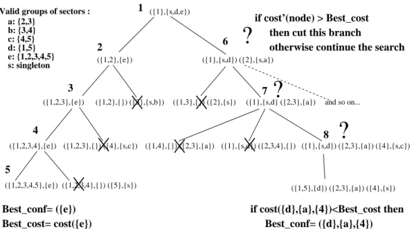
Figure 1 illustrates a tree search that builds all valid combinations of airspace modules, on the same example as before. Here, each tree node is a list of couples where the first element is a group of modules, and the second is the list of valid ATC sectors that contain these modules, but no modules from the other groups of the node.
Valid groups of sectors : a: {2,3} b: {3,4} c: {4,5} d: {1,5} e: {1,2,3,4,5} s: singleton ({1,2,3,4},{e}) ({1,2,3},{}) ({4},{s,c}) ({1},{s,d}) ({2,3,4},{}) ({1},{s,d}) ({2,3},{a}) ({4},{s,c}) ({1,2},{}) ({3},{s,b}) ({1},{s,d}) ({2},{s,a}) ({1,2},{e}) ({1,2,3,4,5},{e})
({1,3},{}) ({2},{s}) ({1},{s,d} ({2,3},{a}) and so on...
({1,4},{}) ({2,3},{a})
({1,5},{d}) ({2,3},{a}) ({4},{s}) ({1},{s,d,e})
({1,2,3,4},{}) ({5},{s}) ({1,2,3},{e})
Figure 1: Exhaustive tree search algorithm for airspace partitioning.
Let us illustrate how this tree is built. The root is a node containing a single group {1}, made of only one module. The possible ATC sectors for {1} are s = {1}, d = {1, 5}, and e = {1, 2, 3, 4, 5}. From this point, we may add a second module, say 2, either in the same group already containing 1 (left branch), or in a new group (right branch). For the left branch ({1, 2}), the only ATC sector containing both 1 and 2 is e. For the right branch ({1} and {2} as separate groups), the list of possible ATC sectors for {1} now contains only s = {1} and d. The ATC sector e is no longer a valid possibility: it contains 1, but also 2 which is already in a separate group. For this group {2}, the valid ATC sectors are s = {2} and a = {2, 3}.
While exploring this tree, it may happen that the list of possible ATC sectors becomes empty. This is the case for example with the node made of groups {1, 2} and {3} (when developing the left branch). There is no valid ATC sector containing both 1 and 2 which does not also contain 3. There is no need to develop further this node, as it will never lead to an operationally valid airspace partition.
The selection of the best airspace partition is made according to the cost criteria defined in section 5.1, which depend on the number of ATC sectors and the values of the probabilities plow, pnormal, and phigh issued by the neural network for each control sector of the considered airspace configuration.
The exhaustive tree search may be computationally intensive, or even not feasible in a reasonable amount of time, when the number of elementary airspace modules and possible ATC sectors is too high.
5.3. Branch & Bound
Let us describe the Branch & Bound algorithm used to build airspace configurations. The main difference with the exhaustive tree search is that, for each node being explored, a lower bound of the costs of all leaves (full configurations) that can be reached from that node is computed. If this lower bound is higher than the cost of the best configuration found so far, then there is no need to continue the search from this node.
Figure 2 shows how the tree is explored, on the same example as in the previous subsection. In the beginning (steps 1 to 4 in the figure), the search is performed like in the exhaustive search, until a first valid configuration is reached (step 5). Afterwards, the best configuration is memorized, together with its cost, and the following nodes are evaluated and compared to this best configuration.
The cost of a node is similar to the cost of a configuration (see subsec-tion 5.1), except that we consider the best possible choice from among all the control sectors associated with each group in the node, so as to provide a lower bound of all full configurations that can be obtained from that node. In the example shown in Figure 2, the cost function for configurations is denoted cost, whereas the cost function for a node is denoted cost0. When evaluating the cost of node [({1}, {s, d}); ({2}, {s, a})] in step 6, we shall take the best possible choice for group {1}, from among singleton s = {1} and valid group d = {1, 5}, and for group {2}, we will choose among sin-gleton s = {2} and valid group a = {2, 3}. Let us say that the best possible choices are d for group {1} and a for group {2}. The node cost cost0([({1}, {s, d}); ({2}, {s, a})]) is then equal to cost([d; a]), the cost of a virtual, and incomplete, configuration containing only these two ATC sec-tors.
Note that choosing the best ATC sector for each group in the node may lead to virtual configurations that are not airspace partitions. In step 8 for example, a virtual configuration with d = {1, 5}, a = {2, 3} and c = {4, 5} is
Valid groups of sectors : a: {2,3} b: {3,4} c: {4,5} d: {1,5} e: {1,2,3,4,5} s: singleton
otherwise continue the search then cut this branch
if cost’(node) > Best_cost ({1,2,3,4},{e}) ({1,2,3},{}) ({4},{s,c}) ({1},{s,d}) ({2,3,4},{}) ({1},{s,d}) ({2,3},{a}) ({4},{s,c}) ({1,2},{}) ({3},{s,b}) ({1},{s,d}) ({2},{s,a}) ({1,2},{e}) ({1,2,3,4,5},{e})
({1,3},{}) ({2},{s}) ({1},{s,d} ({2,3},{a}) and so on...
({1,4},{}) ({2,3},{a}) ({1,5},{d}) ({2,3},{a}) ({4},{s}) ({1},{s,d,e}) ({1,2,3,4},{}) ({5},{s}) 1 2 3 4 5 Best_conf= ({d},{a},{4}) Best_cost= cost({d},{a},{4}) if cost({d},{a},{4})<Best_cost then Best_cost= cost({e}) Best_conf= ({e}) ({1,2,3},{e})
?
6 7 8?
?
Figure 2: Branch & Bound algorithm for airspace partitioning.
not a valid airspace partition as module 5 is in both sectors d and c. However, this heuristic ensures that the cost of a node is always lower than the cost of any valid configuration that can be reached from that node.
6. Predicting airspace configurations throughout the day 6.1. Description of the algorithm
So far, we have seen how a neural network could be used to assess the con-troller workload for any given ATC sector, and how to partition the airspace so as to balance this workload as well as possible among all sectors, at any given time t. Now, let us see how to build an airspace configuration schedule for a whole day of traffic.
Finding an optimal airspace partition of the whole airspace at every mo-ment of the day seems the most straightforward solution, but it would lead to a succession of drastically different configurations in short periods of time. In reality, the airspace is reconfigured around 30 times a day (for French airspace), and usually with relatively minor changes from one configuration to another. The reason is that transferring one or more airspace modules
from one controller to another must be done safely, ensuring that the receiv-ing controller does not miss any potentially dangerous situations in the new traffic and the new airspace sector he will have to handle.
1. Initial configuration (t=0):
1 ATC sector ←− all elementary airspace modules 2. At each time step (1 minute):
• Decide if airspace must be reconfigured −→ check workload in each ATC sector • If so, reconfigure airspace:
– select modules to recombine, – explore all combinations,
– select configuration with minimum cost.
Figure 3: Iterative algorithm for airspace sectors opening schedule.
So it was decided to mimic the actual behaviour of control room man-agers as well as possible, keeping the current airspace configuration as long as it remained acceptable. Figure 3 describes the main loop of the chosen algorithm. The current airspace configuration is checked at every time step. If the workload in some sectors of the current configuration is really too low (plow close enough to 1) or too high (phigh close enough to 1), then a recon-figuration is triggered. Depending on a user-preferred option, either only a few sectors are recombined, or the whole airspace is reconfigured.
Let us recall that the network was trained on observed sector statuses (merged, normally operated, or split). So, when a configuration change is triggered, one might interpret the network output as a recommendation to split or merge the triggering sector. This output is just a workload indication, though, and the tree search algorithm does not restrict itself to splitting or merging sectors: it recomputes a new optimal partition of the set of modules chosen for recombination.
As a result, the transition from one configuration to the next may show split sectors, merged sectors, or modified boundaries between two ATC sec-tors due to the transfer of one or several modules from one sector to the other.
There may be even more complex recombinations such as A, BC, D, E −→ AB, CDE (where A,B,C,D, and E are airspace modules). Some of these complex recombinations may actually not be feasible in operation. In fu-ture work, we plan to optimize sequences of configurations while satisfying constraints on the transitions, allowing for example only one simple change per sector: split, merge, shift boundaries, or open a new sector made up of modules transferred from other sectors.
6.2. Decision criterion
In order to describe more formally the decision criterion triggering the configuration changes, let us consider our three probabilities (plow, pnormal, phigh) sorted by decreasing values p1, p2, p3. The decision criterion is expressed as follows, depending on which probability is the highest:
• if p1 is the probability plow that the workload in the sector is too low: the decision to reconfigure is taken only if 1 − p1 < α
• if p1 is the probability phigh that the workload is too high: we decide to reconfigure only if 1 − p1 < β, where β is a chosen parameter. In the other cases, the sector does not trigger a reconfiguration. We choose different criteria for probabilities plow and phigh, because we may need to be more reactive when the workload is increasing than when it is decreasing. 6.3. Choosing the sectors to recombine
When a reconfiguration is triggered, we can adopt different strategies when building the set of sectors to recombine. We can select either:
• only the triggered sectors (phigh or plow close enough to 1),
• or the sectors for which phigh (or plow) is higher than the other two probabilities. This usually gives us a slightly larger set than with the previous criterion,
• or the previous set to which we add the neighbouring air traffic control sectors. This increases the chances of a better local recombination, especially for under-loaded sectors. These sectors cannot be recombined alone, whereas overloaded sectors can always be split as long as they are made up of several modules,
• or all the sectors. This allows an optimal partition for the whole airspace to be found.
The user can choose one of the above options, or a mix of local and full recombinations. In the latter case, the default behaviour is to make a local recombination (for example only sectors for which the probability phighor plow is the highest), except when there are more than 2 connected components (or a chosen number) in the set of ATC sectors to recombine. In this case, a full airspace reconfiguration is triggered. The rationale underlying this logic is that there are some cases when the limited recombination is not sufficient, for example when there are two under-loaded sectors that are not geographically adjacent.
Sectors can be recombined using either the exhaustive tree search for local recombinations only, or the branch & bound for both local and full reconfigurations. The results presented in this article are obtained with full reconfigurations with the branch & bound. Before presenting these results, let us detail the experimental setup.
7. Experimental setup
7.1. Discussion on the choice of input trajectories
The neural network was trained on actual aircraft trajectories (see details in the next subsection). When trying to forecast airspace configurations, the input trajectories were simulated from flight plans.
Choosing radar tracks to tune the workload model and flight planned tra-jectories to predict future workload may introduce a bias between modelling and forecasting, as the actual trajectories may have changed from the planned trajectories, due the controllers’ actions. With radar tracks, trajectory con-flicts are solved by the controllers before separation losses25 actually occur, whereas this is not the case when using flight plans. So the proximity-related metrics relying on the distance between aircraft, as well as the conflict-related metrics, may be under-estimated when using radar tracks instead of flight planned trajectories.
25In the french upper airspace, and in many other European countries, the horizontal
separation between two aircraft should be at least 5 nautical miles, unless their vertical separation is at least 1000 feet. A ”conflict” occurs when it is expected that the future relative positions will not achieve this separation.
This may have slightly biased the selection of relevant metrics (see sec-tion 3), although the conflict-related metrics that were implemented in our initial set of metrics use relative directions and velocities, so potential con-flicts should be correctly detected with enough anticipation, before trajecto-ries are deviated by the controller. In any case, these biases should remain small, considering the relative influence of conflict-related metrics when com-pared to the aircraft count, the sector volume, and other metrics (see [2] and [3]).
So we use radar tracks for workload modelling, and flight planned tra-jectories for forecasting purposes, as we have no better guess on where the aircraft will be in the future. In future works, a mix of radar tracks and intended26 trajectories may provide greater accuracy. After this discussion on the possible biases due to the chosen input traffic, let us return to the details of our experimental setup.
7.2. Training the neural network on historical data
For the results shown below, the neural network was trained on data sam-ples from 2nd June, 2003, using recorded traffic (”radar” tracks) and sector opening archives from the five French air traffic control centres (ATCCs).
The data set used to train the neural network was built by measuring the relevant complexity metrics every minute of the day, in all ATC sectors of the five centres. The complexity metrics were computed from the aircraft trajectories and sector geometry. The training and test patterns were made from the input complexity metrics and from the observed state of each sector, merged, normal (i.e. actually operated), or split, coded as a state vector (see section 4). Data samples corresponding to a state where the sector is neither operated, nor split into several smaller sectors, nor collapsed within a larger sector were discarded, as we cannot deduce anything on the actual workload from such states.
In our training set, about 46% of the observed patterns fell in the merge class, 27% in the normal class, and 27% in the split class. Detailed results on the neural network outputs can be found in previous publications ([2], [3], [38]). Let us just say that the correct classification rates across all classes were
26”Intended trajectory” can be understood here as the baseline trajectory entered by
the pilot in his flight management system (FMS), and from which he might deviate if instructed to do so by the controller so as to avoid other traffic. It may be different from the flight plan available in ground-based systems, or simply more accurate.
around 85% with a feed-forward neural network with 15 hidden units, when using smoothed input metrics (see [38]). Considering each class individually, we obtained 90% of correct classifications for the merge class, 68% for the normal class, and 93% for the split class. The results on the test set were quite consistent with those obtained on the training set. We have a feeling that these results could still be improved by considering the input metrics as time series and by using recurrent neural networks, but this remains to be done.
7.3. Choice of parameters
Our initial results with a straightforward decision criterion based on the highest probability, and with raw complexity metrics as input showed too frequent configuration changes during the day, although the evolution in the number of ATC sectors stayed fairly close to the actual airspace configura-tions.
The choice of parameters α and β27for the decision criterion was discussed in [36]. The best compromise that was found was α = 0.1 and β = 0.3. These values mean that our algorithms are more reactive when the workload increases than when it decreases. This seems to reflect the controllers’ actual behaviour.
Smoothing the input metrics over 30 minutes with a ”moving average” method also improved the results for an air traffic control centre with large sectors such as Brest ATC centre28. We use these parameters in the results presented in this paper.
7.4. Assessing the airspace configuration on recorded trajectories
In addition to the neural network evaluation, we also need to assess the airspace configurations produced by our algorithms. A first step to validate our approach was to compute the complexity metrics from real recorded traf-fic (”radar tracks”), and compare the resulting configurations to the actual sector openings.
27An additional parameter η expressing a threshold on the difference between the two
highest probabilities was also used in [36]. As this parameter was useless, considering the current values used for α and β, it was abandoned.
28The smoothing strategy may vary from one centre to another: trials with centres
where ATC sectors are smaller seem to show better results with a shorter time window, but no exhaustive results on this subject have been published yet.
Ideally, the computed schedules should reproduce the actual configura-tions recorded that day. However, there is a high variability in the decisions made by control room managers on how to reconfigure the airspace, which comes in addition to the variability of decisions on when to reconfigure. We may hope that our workload model could give an indication on when to trigger a reconfiguration and allow the tree search method to build realis-tic configurations, but our algorithms may not compute exactly the same configuration as in reality.
So we will mainly assess the realism of the computed schedule by com-paring the number of ATC sectors in our computed configurations with the actual number of sectors open on the same day. Pearson’s correlation coeffi-cient may give an indication of the linear correlation between the computed and the real number of sectors. However, this may not always be reliable29 so we will also compute an ad-hoc ”dissimilarity measure”, which is the sur-face delimited by the two curves (computed and real number of ATC sectors operated during the day), divided by the surface between the x-axis and the curve of the real number of ATC sectors. With this measure, two identical curves have a dissimilarity 0 if they are exactly superposed. In addition, we will also consider the number of reconfigurations throughout the day, which should be close enough to the real one.
7.5. Assessment of the airspace configuration forecasted from planned traffic Radar tracks are available only after the aircraft have flown through the airspace. The proposed algorithms may be useful only if we are actually able to forecast airspace configurations before the aircraft enter the airspace.
For this purpose, predicted aircraft trajectories are simulated from the anticipated traffic demand (i.e. flight plans filed by the airline operators), using a fast-time simulator (see [39], [40]). The resulting airspace configu-ration schedule is then compared both to the prediction that was made the day before by flow management, and to the actual sector openings. Let us now see a few results, starting with the validation on historical data.
29The correlation coefficient between two equal variables x and y = x will be 1. Let us
note however that this coefficient is not sufficient actually to measure how close we are to equality: the correlation coefficient between a variable x and another variable y = x + d, where d is a constant offset, will also be 1.
0 5 10 15 20 0 200 400 600 800 1000 1200 1400 -20 0 20 40 60 80 100 120
Nb. control sectors Number of aircraft
Time (minutes)
Real configurations Computed configurations Real traffic (radar tracks)
Figure 4: Computed vs. real configurations (Brest ACC, 6th June 2003), using real traffic as input.
8. Results
8.1. Comparison to real configurations, using recorded traffic
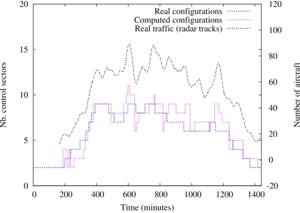
The model tuned on 2nd June was tested on two other days of traffic, using recorded radar tracks as input. Figure 4 shows the number of air traffic control sectors in the computed configurations, and the real number of ATC sectors that were open on 6th June 2003, in Brest air traffic control centre. The upper curve shows the number of aircraft within the centre boundaries, as an indication of the total traffic that day. Note that this curve is related to the y axis on the right, and that it has been shifted upward so as to make the figure more readable. The left y axis shows the number of sectors, and the x axis is the time, expressed in minutes after 0h00.
As shown on this figure, the computed number of sectors is fairly close to the actual number of sectors that were operated that day. The dissimilarity
measure is 0.191 and Pearson’s correlation coefficient is 0.91. Our algorithms found 46 configuration changes, whereas there were 33 in reality.
The total number of aircraft within the centre (upper curve) is given as a very crude indication of the overall workload. We can observe that the number of ATC sectors follows this curve more or less, although not always strictly. One should bear in mind that the traffic may be dispatched differently across the sectors throughout the day, and also that the number of aircraft is not the only factor of air traffic complexity and workload. Still, this traffic curve gives a good hint of the traffic variations throughout the day, and allows finer interpretations of the other curves.
0 5 10 15 20 0 200 400 600 800 1000 1200 1400 -20 0 20 40 60 80 100 120
Nb. control sectors Number of aircraft
Time (minutes)
Real configurations Computed configurations Real traffic (radar tracks)
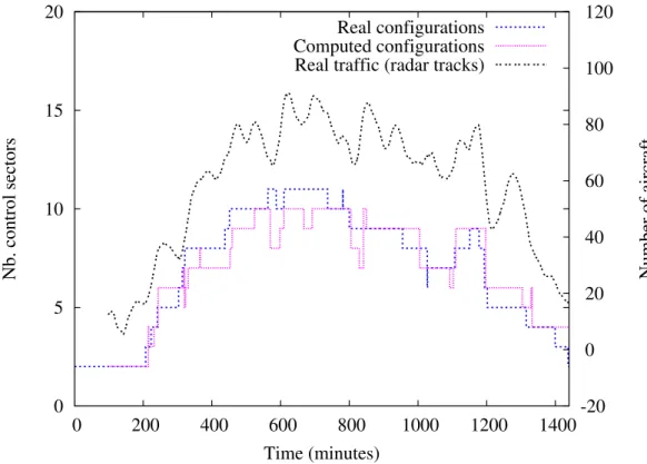
Figure 5: Computed vs. real configurations (Brest ACC, 7nd June 2003) using real traffic as input.
Figure 5 shows the same information, but for 7th June 2003. For that day, the algorithms show slightly better results, with a dissimilarity mea-sure of 0.115 and a correlation coefficient of 0.94. There were 37 computed configurations, against 33 in reality.
The two figures, 4 and 5, illustrate the fact that the model only reflects the average behaviour of air traffic controllers and control room managers when they decide to split or merge sectors, or reconfigure otherwise. There are variations in this behaviour among the population. Some controllers are more experienced or more efficient than others and may consequently manage higher workloads, or there may be younger controllers completing the final period of their training under the supervision of fully qualified instructors. 8.2. Planned vs. real 0 5 10 15 20 0 200 400 600 800 1000 1200 1400 -20 0 20 40 60 80 100 120
Number of control sectors
Number of aircraft
Time (minutes)
Planned traffic (initial traffic demand) Configurations with planned traffic Real traffic (radar tracks) Configurations with real traffic
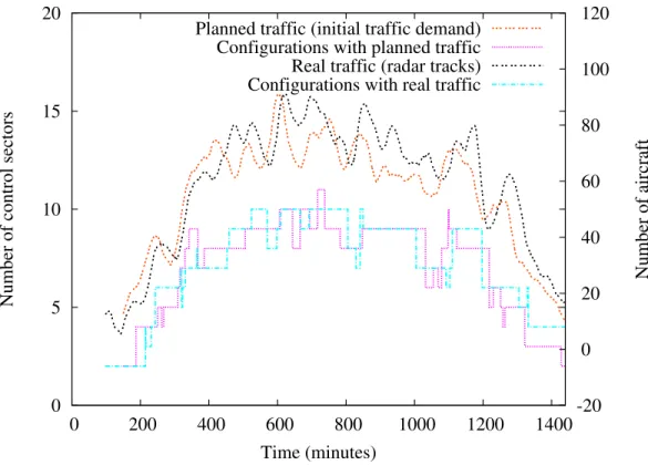
Figure 6: Initial traffic demand (flight plans) vs. real traffic (radar tracks), in Brest ACC on 7th June 2003.
Figure 6 shows the traffic in Brest airspace on 6th June 2003, and the number of ATC sectors in the configurations computed with either the real traffic or the simulated traffic as input. In the latter case, a fast-time30 air
com-traffic simulator was used to compute the aircraft trajectories from the flight plans of the initial traffic demand. This is typically what might be done in a pre-tactical context, well before flights take off, when no radar tracks are available.
We can observe the differences between the planned traffic and real traf-fic by considering the two upper curves in Figure 6. Although it may be described as a statistical phenomenon ([47]), this difference between planned and real traffic is rather difficult to anticipate with great accuracy in a given sector at a given time. This leads to uncertainties when forecasting the com-plexity metrics used as input to the neural network.
Missing flight plans or short-notice departures may indeed lead to drasti-cally under-estimated aircraft counts and other complexity metrics (see [22]), especially for departure sectors. Considering the results in Figure 6, this does not seem to be the case with our flight plan data and with the considered en-route ATCC. However, we still observe some differences that may stem from navigation uncertainties, re-routings, flight cancellations, etc. These uncertainties on planned traffic do have an influence on the quality of the forecast, although this influence is certainly somewhat lessened by the use of a moving average method to smooth the input metrics.
Flight planning uncertainties may be reduced by using a mix of radar tracks and flight intentions, if the proposed algorithms are to be used in a tactical context where complexity metrics are forecast 20-30 minutes ahead. In any case, the difference between planned traffic and actual traffic may be an important source of error. The quality of the prediction depends on the reliability of the 4D-trajectory forecast.
8.3. Comparison with the current forecast
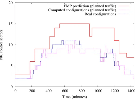
Let us now compare our forecast, using planned traffic, with the actual prediction made on the same data by the flow management operators. We can see in Figure 7 that the schedule computed with planned traffic as input is much closer to the number of control sectors that were actually open that day than what was predicted by the FMP operators from the same flight plans that we used.
The dissimilarity metric measuring the difference between prediction and reality is 0.568 for the FMP schedule, whereas it is only 0.137 for our
0 5 10 15 20 0 200 400 600 800 1000 1200 1400 Nb. control sectors Time (minutes)
FMP prediction (planned traffic) Computed configurations (planned traffic) Real configurations
Figure 7: Airspace configuration forecast using flight plans as input: computed prediction vs. current FMP prediction (Brest ACC, 7th June 2003).
cast31.
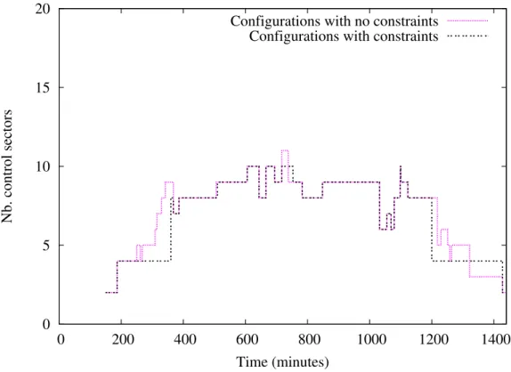
8.4. Results with or without constraints on the number of sectors
0 5 10 15 20 0 200 400 600 800 1000 1200 1400 Nb. control sectors Time (minutes)
Configurations with no constraints Configurations with constraints
Figure 8: Airspace configuration forecast with or without constraints on the maximum number of ATC sectors (Brest ACC, 7th June 2003).
Finally, let us illustrate what may be the most useful application of the proposed algorithms. So far we have not introduced constraints on the max-imum number of ATC sectors in each configuration. Running the algorithms without such constraints allows the operator to check if the duty roster is sufficient to handle the planned traffic.
Now, what happens if for some reason, there are not enough controllers, or not enough working positions available to handle the traffic? In such cases,
31The correlation coefficient is 0.91 for the FMP prediction and 0.93 for our prediction,
the cost comparison described in section 5.1 allows the branch & bound algo-rithm to find configurations that satisfy such constraints while balancing the workload as well as possible. In Figure 8, we have constrained the maximum number of control sectors to 4 between 00h00 and 06h00, 8 between 06h00 and 08h30, 10 between 8h30 and 20h00, and finally 4 after 20h00. The figure shows the number of sectors for both solutions, with or without constraints.
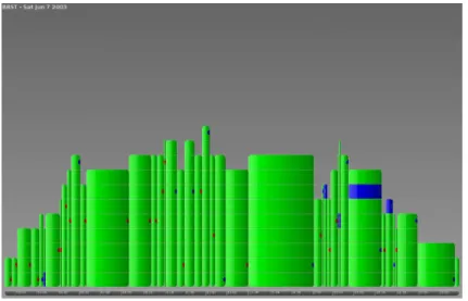
Figure 9: HMI display of the airspace configuration forecast, without constraints (Brest ACC, 7th June 2003).
An experimental human-machine interface is currently under develop-ment, with the aim of demonstrating and refining the proposed algorithms. Figure 9 shows the general view of the sector opening schedule for Brest centre, without constraints, over one day of traffic. Each column represents a partition of the airspace into ATC sectors. A pop-up window (not shown) may give more details on each configuration when browsing over the coloured boxes. The colour code is the following: blue when the sector is under-loaded, green when it is normally loaded, red when it is overloaded (although there are none here, without constraints). Coloured dots on the right of each box give an indication of which workload threshold (low or high) triggered the configuration change.
When posting no constraints on the maximum number of sectors, this display shows how many sectors would be necessary to handle a given traf-fic demand. This could allow the staff manager to adapt the duty roster to the input traffic. Note that without constraints, only ATC sectors made
up of a single airspace module can be overloaded: otherwise a sector com-posed of several modules would have been split into two smaller sectors when becoming overloaded.
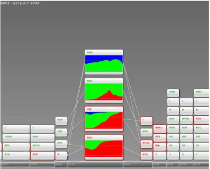
Figure 10: HMI display of the airspace configuration forecast, with constraints (Brest ACC, 7th June 2003).
Figure 10 shows the same situation, with constraints on the maximum number of sectors. We can observe the overloaded control sectors shown in red. Such a display could help flow managers to take preventive measures (departure delays, reroutings) so as to prevent such dangerously overloaded situations from actually occurring.
The user can switch to a more detailed view, as shown in Figure 11 where the workload evolution across time is displayed for each selected sector. For this purpose, each selected sector box shows the three probabilities issued by the neural network, stacked one above the other, using the same colour code: blue for plow, green for pnormal, and red for phigh. The transitions between airspace configurations are also shown.
9. Conclusion and perspectives 9.1. Summary remarks
Forecasting airspace configurations requires at least two things: first a model assessing the controller workload for any given ATC sector in traf-fic conditions of variable complexity, and second an algorithm providing an optimal partition of the airspace into ATC sectors.
Figure 11: Details of some overloaded control sectors when enforcing constraints on the number of available working positions (Brest ACC, 7th June 2003).
The proposed workload model assumes that the observed sector opera-tions reflect the controllers’ actual workload: ATC sectors made of several modules may be recombined when the workload is either too high or too low. The model relies on a neural network to issue workload probabilities, using the sector volume and a selection of air traffic complexity metrics as input. Among several others found in the literature, these metrics appeared to be the most correlated to the observed sector status in past operations. Some others also proved relevant but were redundant with the selected variables and slightly less relevant. As the literature is fairly extensive on this subject, we have not implemented all existing metrics, and other complexity factors may be tried in the future that might improve the model.
The partitioning problem, which is highly combinatorial when considering all the possible combinations of airspace modules, has been addressed using standard tree search methods. This was made possible by restricting the tree search to partitions made up only of ATC sectors described in the ATCC databases. The neural network output probabilities were used to assess the cost of candidate configurations while exploring the tree.
comparing the results to the archived sector openings. The neural network was trained on data collected in the five French ATC centres on 2nd June 2003 and assessed on two other days (6th and 7th June 2003). Two measures were used to quantify the differences between the computed output and reality: a dissimilarity measure accounting for the differences in the number of ATC sectors, and the number of configuration changes.
The proposed method showed that the number of ATC sectors was fairly close to the actual one. The dissimilarity measure was 0.191 on 6th June and 0.115 on 7th June. However, the number of configuration changes was still above what actually occurred in reality: 46 against 33 in reality on 6th June, and 37 against 33 on 7th June.
After outlining the possible sources of bias and forecasting errors that may occur due to the difference between the planned traffic demand and actual flights, we tried our algorithms on simulated trajectories computed from flight plans. The comparison to the actual forecast made by the flow management operators shows that our prediction is far more realistic than those done currently in operations: the dissimilarity measure is 0.137 for the computed configurations, and 0.568 for the FMP forecast on 7th June. 9.2. Limitations of the proposed method
In our results, the influence of flight planning and navigation uncertainties was certainly somewhat lessened by two factors. First by the use of a moving average method to smooth the input metrics (including the aircraft count), and second by the fact that the neural network trained on historical data reflects the average behaviour of controllers and control room managers over the observed past airspace operations.
Concerning the first factor, one must be aware that there is a trade-off between smoothing the metrics and the forecast accuracy. In fact, averaging the metrics over too long a period delays the times when airspace configu-ration changes are predicted. This might motivate further research, using time series, instead of smoothing the input metrics with a moving average method.
Dealing with flight planning uncertainties may have an influence over the context in which the proposed algorithms could be used. A certain level of uncertainty and the use of smoothed metrics may be acceptable in a pre-tactical context, when roughly assessing how many ATC sectors are necessary to handle the planned traffic. But this same level of uncertainty may not be acceptable for a tactical tool, when overloads need to be anticipated with