HAL Id: inria-00331772
https://hal.inria.fr/inria-00331772
Submitted on 17 Oct 2008
HAL is a multi-disciplinary open access
archive for the deposit and dissemination of
sci-entific research documents, whether they are
pub-lished or not. The documents may come from
teaching and research institutions in France or
abroad, or from public or private research centers.
L’archive ouverte pluridisciplinaire HAL, est
destinée au dépôt et à la diffusion de documents
scientifiques de niveau recherche, publiés ou non,
émanant des établissements d’enseignement et de
recherche français ou étrangers, des laboratoires
publics ou privés.
An algorithm to map asymmetries of bilateral objects in
point clouds
Benoît Combès, Robin Hennessy, John Waddington, Neil Roberts, Sylvain
Prima
To cite this version:
Benoît Combès, Robin Hennessy, John Waddington, Neil Roberts, Sylvain Prima. An algorithm
to map asymmetries of bilateral objects in point clouds. 5th IEEE International Symposium on
Biomedical Imaging: From Nano to Macro (ISBI’2008), May 2008, Paris, France. pp.1139-1142,
�10.1109/ISBI.2008.4541202�. �inria-00331772�
AN ALGORITHM TO MAP ASYMMETRIES OF BILATERAL OBJECTS IN POINT CLOUDS
Benoˆıt Comb`es
1,2,3, Robin Hennessy
4, John Waddington
4, Neil Roberts
5and Sylvain Prima
1,2,31INSERM, U746, Facult´e de M´edecine CS 34317, F-35043 Rennes Cedex, France 2INRIA, VisAGeS Unit´e/Projet, F-35042 Rennes, France
3Univ. Rennes I, CNRS, UMR 6074, IRISA, F-35042 Rennes, France 4RCSI, St Stephens Green, Dublin 2, Ireland
5MARIARC, University of Liverpool, Pembroke Place, Liverpool, L69 3GE, UK
ABSTRACT
We present a method to automatically quantify the local asymme-tries of bilateral structures in point clouds. The method relies on the robust computation of the approximate symmetry plane of the object under study. This plane is defined as the minimiser of a crite-rion, based on a M-estimator and devised to reduce the influence of asymmetrical features of the object. An algorithm is then proposed to minimise this criterion. Once the algorithm has converged, the residual distances between the points and their symmetrical counter-parts quantify the local asymmetries, yielding a 3D asymmetry map. We show the algorithm to be accurate, with a high capture range, on an ideal, perfectly symmetrical dataset. We investigate its robustness and accuracy properties on highly corrupted datasets. We also evalu-ate the accuracy of the obtained 3D maps using ground truth datasets where the asymmetries are known. Finally, we propose several orig-inal applications of this method on real data.
Index Terms— Symmetry, Asymmetry, Point clouds, Surfaces, 3D mapping, Face, Skull
1. INTRODUCTION
The advent of high resolution 3D techniques to image the human body has allowed the development of numerous automated tech-niques for morphometric studies. Accurate, robust and reproducible methods for in vivo measurement of volumes, shapes, lengths, etc, are often crucial for a good assessment of normal as well as patho-logical conditions. Quantification and localisation of asymmetries are particularly relevant when dealing with brain images, and many methods have been devised for this purpose [1, 2]. These tech-niques deal with grey level images, and allow to assess brain asym-metries on a voxel-by-voxel basis. To our knowledge, there exists no such method for landmark-free, local quantification of asymme-tries in point clouds. Point clouds are often met in medicine, ei-ther by directly scanning the object of interest or by extraction of points/surfaces from 3D grey level images. These point clouds are 3D geometrical representation of structures of interest such as the face, the inner/outer surface of the skull, the inner/outer boundary of the brain cortex, etc. Localising and quantifying the asymmetries in point clouds is relevant in many medical applications, for instance:
⊲ In maxillo-facial reconstructive surgery, measuring asymme-tries is crucial during pre-operative planning. Typically, it can be done by extracting the patient’s skull or face from CT images, cor-recting the asymmetries in the resulting 3D surface, and building a virtual model of the required structures. This model can then be
used to build implants or a real template (by stereolithography) to reconstruct the affected side [3, 4].
⊲ Paleoneurology is based on the idea that it is possible to study the brain indirectly by analysing fossil remains [5]. Typically, these studies rest on the observation of fossil endocranial casts (or endo-casts), that are natural molds of the inner skull. The main features of the brain being partially imprinted on the inner surface of the skull, it is possible to draw inferences on the brain (shape, size, asymmetries, etc.) by looking at such endocasts. Direct CT scanning of the skull also allows the extraction and analysis of its inner surface. These techniques should help to answer whether some gross asymmetries (planum temporale, Yakovlevian torque) usually met in Modern Hu-mans are reduced or absent in Archaic HuHu-mans, other human lin-eages and in other great apes.
⊲ Reduction (or reversal) of brain anatomical asymmetries has been previously reported in schizophrenia [6]. Recent works sug-gest that subtle facial dysmorphologies, and potentially asymme-tries, could be also present in this disease [7, 8]. Measuring asym-metries in face data and looking for correlation with indices of brain function (such as cognition) could thus help supporting (or rejecting) the neurodevelopmental hypothesis of schizophrenia.
Localisation and quantification of asymmetries of bilateral ob-jects implicitly rely on the definition of a proper sagittal (or mid-facial) plane diving the structure of interest into two similar parts, and then measuring departures from perfect symmetry. Comput-ing this plane is challengComput-ing, because the object under study (brain, skull, face) is only grossly symmetrical in practice.
Two main approaches have been proposed to compute automati-cally the symmetry axis/plane of bilateral objects in point clouds. In a first approach, the symmetry plane is built via the extended Gaus-sian image (EGI) of the cloud [9, 10]. However, practically this method is dedicated to convex structures for which a neighbourhood notion can be derived and is not robust to important occlusions. In a second approach [11, 4, 12], the symmetry plane is estimated us-ing a two-step algorithm that consists in a rigid-body registration followed by a plane extraction. However, computing the symme-try plane from the optimal rigid-body transformation is an ill-posed problem that needs ad hoc choices leading to different solutions.
In this paper, we propose an original approach to estimate di-rectly the plane (i.e. without relying on an intermediate rigid-body transformation) minimising a robust criterion that allows to take into account only highly symmetrical features of the object. The algo-rithm is presented in Section 2. Its capture range, robustness and ac-curacy are investigated in Section 3. In Section 3.3, we show some results on real (face, skull, endocranial) data. Finally, we conclude and give some perspectives in Section 4.
2. METHODS 2.1. A robust criterion
Without loss of generality, we consider in the rest of this article that the object under study is represented by a cloud of points noted O, withcard(O) = N . For an ideal bilateral object having a perfect symmetry, there exists a symmetry plane P superposing each point with its counterpart in the other side of the object. We note SP the
symmetry (reflection) with respect to P . The fact that P is a perfect symmetry plane simply writes:
∀xi∈ O, ∃yi∈ O such that yi= SP(xi) (1)
However, the object under study is rarely perfectly symmetrical. A possible way to circumvent this problem is to define an approxi-mate symmetry plane ˜P as:
˜
P= arg min
P,y1,...,yN
= X
i=1,...,N
ρ(||yi− SP(xi)||) = arg min P,y1,...,yN
EP
(2) where y1, . . . , yNbelong to the cloud O and ρ: IR+ → IR+is an
increasing function favouring the pairs(xi, yi) with low residuals.
Indeed, an accurate symmetry plane estimation must only rely on the highly symmetrical features of the objects. A suited function ρ will be proposed and explicited in Section 2.2. It is easy to check that if ρ(0) = 0, this criterion is equal to zero (thus minimal) in case of a perfect symmetry plane P by choosing yi= SP(xi).
2.2. Algorithm
To our knowledge, there is no closed-form solution for Problem 2. Thus, we devise the following iterative algorithm, inspired by the ICP algorithm [13] and called SPE (Symmetry Plane Estimation). It can be easily shown to converge to a (at least local) minimum ofEP:
Step 0: Initialise ˜P
Step 1:y˜1, ..,y˜N= arg miny1,...,yN
P
i=1,...,Nρ(||yi− SP˜(xi)||)
Step 2: ˜P = arg minP
P
i=1,...,Nρ(||˜yi− SP(xi)||)
Step 3: if ˜P has changed go to Step 1 else finish
⊲ Solving Step 1
One has to find N pointsy˜iin O so as to minimiseEP while P
is kept fixed. The trivial solution to Step 1 is to simply choosey˜ias
the closest point of SP(xi) in O.
⊲ Solving Step 2
The goal of ρ is to limit the influence of the pairs with high resid-uals. If ρ is chosen as an M-estimator [14], Step 2 can be rewritten:
˜ P = arg min P X i=1,...,N wi||˜yi− SP(xi)||2 (3) where wi= ρ′(||˜y i− SP(xi)||) 2||˜yi− SP(xi)|| (4) Given that the weights wi depend on the residuals ri =
||˜yi − SP(xi)||, which in turn depend on the plane P , there is
no closed-form solution for Eq. 3. We use an iteratively reweighted least-squares scheme [15], that can be shown to converge. Its princi-ple is to alternatively update the weights withanks to Eq. 4 (with P
fixed) and solve Eq. 3 with respect to P (with the weights wifixed).
This last problem can be solved using the following theorem, that we prove in another paper [16].
Parameterization : We characterise the plane P using its unit nor-mal n and its distance to the origin d which leads to (I3being the
3 × 3 identity matrix). Then, it can be easily shown that: SP(xi) = (I3− 2nnT)xi+ 2dn (5)
Theorem : For given sets of points{x1, ..., xN}, {yi, ..., yN} and
a given set of associated weights{wi} (independent of P ), the
plane P = (d, n) that minimises X i=1,...,N wi ˛ ˛ ˛ ˛yi− S(d,n)(xi) ˛ ˛ ˛ ˛ 2 (6) is characterised by:
• n colinear with the eigenvector corresponding to the smallest eigenvalue of the matrix A∈ IR3, where
A= X i=1,...,N wi[(xi− xg+ yi− yg)(xi− xg+ yi− yg)T − (xi− yi) (xi− yi)T] with xg = P i=1,...,Nwixi P i=1,...,Nwi and yg= P i=1,...,Nwiyi P i=1,...,Nwi . • d = 1 2(xg+ yg) Tn.
In practice, we choose ρ as the Leclerc function, which gives: wi(ri) = 1 σ2exp − r2 i σ2
This function allows an implicit modelling of the image noise, as wi(ri) is proportional to the probability density function of a white
noise of standard deviation σ. 2.3. Implementation details
⊲ Initialisation: The plane initialising SPE is computed using the principal axes and the centre of mass of an uniformly resampled version of O [10].
⊲ Refinement of the solution: Criteria based on closest point matching are often affected by local minima very close to the global minimum [17]. To overcome this problem, we run SPE from the initial estimate until it converges. Then, considering that the global minimum is very close (or even equal in some cases) to the found minimum, we apply a small random perturbation on the latter in or-der to leave the area of local minimum convergence, and rerun SPE from this new initial estimate. This process is repeated five times and the solution giving the smallest criterion is likely to correspond to the global optimum ofEP [17].
⊲ Multiscale and multiresolution scheme: The convergence of SPE is very dependent on σ. In essence, a large σ allows good ro-bustness, and a small σ allows a good accuracy. Thus, to allow both accuracy and robustness, we view σ as a scale parameter and run sev-eral successive SPE with decreasing σ values (in practice, σ = 50, 10, 5 and 0.5). At the beginning of this multiscale scheme, large values of σ only lead to a gross estimation of the unknown plane. Consequently, it is useless to take the entire point set O into account at these stages. As a result, we propose a coarse-to-fine approach, where the cloud O is decimated at large σ values, and then refined progressively when σ decreases. In the following, we will note SPE2
this multiscale SPE algorithm and SPE1 the standard SPE with a
⊲ Fast searching method: The closest point searching uses a Kd-Tree subdivision of the 3D space.
⊲ Stopping criterion: We choose as ad hoc stopping criterion ||Pt− Pt−1|| ≤ 0.01 where Pt= (n, d)t
is the searched plane P at the end of iteration t.
The run time of SPE2on a cloud of about 80.000 points is 2 min. on
a PC with an Intel Core Duo T7700 at 2.4GHz with 2GB Ram. 2.4. Asymmetry quantification
Once SPE has converged and a symmetry plane P has been esti-mated, we compute the distance between each point SP(xi) (xi ∈
O) and its closest point yiin O. This distance quantifies the local
asymmetry at xiand is noted ˜A(xi).
3. EVALUATION AND RESULTS 3.1. Evaluation on symmetrical data
We investigate the accuracy and capture range of SPE2on perfectly
symmetrical data. For this, we work on a synthetic perfectly sym-metrical face data of about 80.000 points built from real data (see Sec. 3.3). We apply a few thousand random angular offsets between 0 and 40 degrees and linear offsets between 0 and 60 mm to the ground truth symmetry plane and use it to initialise SPE2. After
con-vergence, we compute the angular and linear errors (that we will call respectively θ and τ ) of the estimated plane compared to the ground truth solution. This experiment shows that for large linear (below 80 mm) and angular (below 31 degrees) offsets, SPE2always converges
to a plane for which θ and τ are less than10−2.
3.2. Evaluation on asymmetrical data
We evaluate the robustness and accuracy of asymmetry quantifica-tion on synthetic data. For this purpose, we add artefacts to a sym-metrical image, whose symmetry plane is still considered as the ground truth. We generate artefacts as follows:
⊲ Occlusions are generated by removing a given quantity of ad-jacent points. In the following, we term outliers the points with no symmetrical counterpart resulting of this removal.
⊲ Asymmetries are generated by applying smooth deformations (Gaussian-like) of strength K and of extent v.
By randomly combining these artefacts, we generate a set of 150 images with varying levels of artefacts. The parameters are chosen such that: (K, v) ∈ [0, 20]2 (one deformation on the right cheek
and another on the right forehead), 0 to 20% of outliers and noise variance ǫ = 0.3. Then the ground truth plane and ground truth asymmetries (as generated by the deformations) are compared.
To assess the accuracy of asymmetry quantification, we devise a global measure of the error E on asymmetries as:
E= 1
N X
i=1,...,N
H(i)|A(xi) − ˜A(xi)|
where A(xi) and ˜A(xi) are respectively the real and the measured
asymmetry amplitude (in mm) and H(i) is an indicative function equal to1 if xias a real bilateral counterpart and0 if it is an outlier.
Tab. 1 shows statistics on τ , θ and E over the 150 experiments and Fig. 1 compares the mapping of asymmetries on one of the im-ages of the dataset using the principal axes (PA), SPE1and SPE2. PA
fails to conveniently locate and quantify asymmetries, whereas SPE1
PA SPE1 SPE2 maximal(τ, θ) error (11.23,10.23) (4.50,2.32) (0.51,0.54) mean(τ, θ) error (8.32,6.61) (0.81,0.62) (0.07,0.22) variance(τ, θ) error (6.23,6.12) (0.82,0.11) (10−3,0.01) maximal E error 7.25 2.84 0.54 mean E error 4.51 1.15 0.32 variance E error 2.37 0.47 0.01
Table 1. Statistics on(τ, θ) and E for PA, SPE1and SPE2
Fig. 1. Top row (left): Face with two deformations K= 15, v = 15, 5% of occlusions and ǫ= 0.3; (right) Mapping of the deformations (i.e. ground truth asymmetries). Middle row (left to right): Mapping of the asymmetries for PA, SPE1 and SPE2. Bottom row (left to
right): Mapping of errors|A(xi) − ˜A(xi)| for PA, SPE1and SPE2.
qualitatively picks up the right areas (cheek and forehead) with un-derestimated asymmetries, and false negatives (nose). SPE2shows
very good accuracy. However, areas with high gradient amplitudes (such as the mouth corner) show a slight error.
3.3. Results on real data
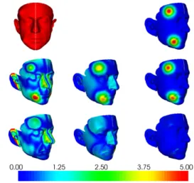
⊲ Face data: A population of 131 healthy subjects, 49 males (mean age of 33.1 years, 22 to 65 years) and 82 females (mean age 32.2 of years, 22 to 59 years) has been face scanned with a portable hand-held laser scanner with resolution and accuracy below 1 mm (Polhemus FastScan, Polhemus Inc, VT, USA, fastscan3d.com). Each of these point sets contains about 80.000 points. We display the asymmetry maps of eight subjects on Fig. 2.
⊲ Skull data: The outer surface of the skull of the Chapelle-aux-Saints Man (Homo neanderthalensis) was extracted from a CT im-age (courtesy of the FOVEA Project: foveaproject.free.fr) using thresholding and morphological operations and contains about 250.000 points. We display its asymmetry map on Fig. 3.
⊲ Endocranial data: A virtual endocast was obtained by laser scanning the natural endocast of a hominid. The cloud contains about 30.000 points. We display its asymmetry map on Fig. 4.
4. DISCUSSION AND CONCLUSION
In this paper we have presented an original formulation for the prlem of estimating the approximate symmetry plane of bilateral ob-jects in point clouds. We have provided an iterative algorithm to
Fig. 2. Asymmetry maps on faces. Four females (top) and four males (bottom). Blue (resp. red) corresponds to symmetrical (resp. asymmetrical) areas. We are currently implementing methods for the statistical analyses of the male-female differences.
Fig. 3. Asymmetry map on a skull. Different views. Strong lat-eral asymmetries can be seen, but the question whether these asym-metries are biologically meaningful or the consequence of the skull being buried in sediments for ages is debatable.
Fig. 4. Asymmetry map on an endocast. Different views. Strong asymmetries can be seen in the fronto-temporal and occipital re-gions, that could relate to the Yakovlevian torque often seen in the brain [6].
compute this plane and evaluated its robustness, accuracy and cap-ture range properties on symmetrical and asymmetrical data. We are currently implementing methods for the normalisation of the sub-jects in a common coordinate system to allow the assessment of the mean asymmetry within a population (ex: males) or the difference of asymmetries between populations (ex: males vs females, con-trols vs schizophrenic patients) using suited point-to-point statisti-cal analysis. Further work will consist in comparing these tech-niques with landmark-based methods, that use geometric morpho-metrics [18, 19, 8]. At last, we will also investigate more sophisti-cated approaches (for instance dense registration with regularisation
constraints) for improved asymmetry mapping. 5. REFERENCES
[1] J.-P. Thirion et al. “Statistical analysis of normal and abnormal dissymmetry in volumetric medical images,” Medical Image Analysis, vol. 4, no. 2, pp. 111–121, June 2000.
[2] C.D. Good et al. “Cerebral asymmetry and the effects of sex and handedness on brain structure: a voxel-based morphomet-ric analysis of 465 normal adult human brains,” NeuroImage, vol. 14, no. 3, pp. 685–700, Sept. 2001.
[3] T.-Y. Wong et al. “Comparison of 2 methods of making sur-gical models for correction of facial asymmetry,” J Oral Max-illofac Surg, vol. 63, no. 2, pp. 200–208, Feb. 2005.
[4] E. De Momi et al. “Automatic extraction of the mid-facial plane for cranio-maxillofacial surgery planning,” Int J Oral Maxillofac Surg, vol. 35, no. 7, pp. 636–642, July 2006. [5] E. Bruner, “Geometric morphometrics and paleoneurology:
brain shape evolution in the genus Homo,” J. Hum. Evol., vol. 47, pp. 279–303, 2004.
[6] T.J. Crow, “Schizophrenia as a failure of hemispheric domi-nance for language,” Trends Neurosci, vol. 20, pp. 339–343, 1997.
[7] A. Lane et al. “The anthropometric assessment of dysmorphic features in schizophrenia as an index of its developmental ori-gins,” Psychol Med, vol. 27, no. 5, pp. 1155–1164, Sept. 1997. [8] R.J. Hennessy et al. “Facial shape and asymmetry by three-dimensional laser surface scanning covary with cognition in a sexually dimorphic manner,” J Neuropsychiatry Clin Neurosci, vol. 18, no. 1, pp. 73–80, 2006.
[9] G. Pan et al. “Finding symmetry plane of 3D face shape,” in IEEEICPR. 2006, pp. 1143–1146.
[10] C. Sun and J. Sherrah, “3D symmetry detection using the ex-tended gaussian image,” in IEEEPAMI, vol. 19, no. 2, pp. 164– 168, 1997.
[11] L. Zhang et al. “3D face authentication and recognition based on bilateral symmetry analysis,” The Visual Computer, vol. 22, no. 1, pp. 43–55, 2006.
[12] H. Zabrodsky et al. “Symmetry as a Continuous Feature,” IEEEPAMI, vol. 17, no. 12, pp. 1154–1166, Dec. 1995. [13] P. Besl and N. McKay, “A method for registration of 3-D
shapes,” IEEEPAMI, 14(2):239–256, Dec. 1992. [14] P.J. Huber, Robust statistics, 1981.
[15] P.W. Holland and R.E. Welsch, “Robust regression using itera-tively reweighted least-squares,” Commun. Statist., vol. 6, pp. 813–827, 1977.
[16] B. Comb`es et al. “Automatic symmetry plane estimation of bilateral objects in point clouds,” IEEECVPR, 2008. In press. [17] D. Simon, Fast and accurate shape-based registration, Ph.D.
thesis, Robotics Institute, Carnegie Mellon University, Pitts-burgh, USA, Dec. 1996.
[18] K.V. Mardia, et al. “Statistical assessment of bilateral symme-try of shapes,” Biometrika, vol. 87, no. 2, pp. 285–300, 2000. [19] C. P. Klingenberg et al. “Shape analysis of symmetric
struc-tures: quantifying variation among individuals and asymme-try,” Evolution Int J Org Evolution, vol. 56, no. 10, pp. 1909– 1920, Oct. 2002.