Adaptive filtering to reduce global interference in evoked
brain activity detection: a human subject case study
The MIT Faculty has made this article openly available.
Please share
how this access benefits you. Your story matters.
Citation
Zhang, Quan, Emery N. Brown, and Gary E. Strangman. “Adaptive
Filtering to Reduce Global Interference in Evoked Brain Activity
Detection: a Human Subject Case Study.” Journal of Biomedical
Optics 12, no. 6 (2007): 064009. © 2007 Society of Photo-Optical
Instrumentation Engineers
As Published
http://dx.doi.org/10.1117/1.2804706
Publisher
SPIE
Version
Final published version
Citable link
http://hdl.handle.net/1721.1/87659
Terms of Use
Article is made available in accordance with the publisher's
policy and may be subject to US copyright law. Please refer to the
publisher's site for terms of use.
Adaptive filtering to reduce global interference in
evoked brain activity detection: a human subject
case study
Quan Zhang
Massachusetts General Hospital Harvard Medical School Neural Systems Group
13th Street, Building 149, Room 2651 Charlestown, Massachusetts 02129
Emery N. Brown
Massachusetts General Hospital
Department of Anesthesia and Critical Care Harvard-MIT Division of Health Sciences and
Technology
Massachusetts Institute of Technology Department of Brain and Cognitive Sciences Boston, Massachusetts 02114
Gary E. Strangman
Massachusetts General Hospital Harvard Medical School Neural Systems Group
13th Street, Building 149, Room 2651 Charlestown, Massachusetts 02129
Abstract. Following previous Monte Carlo simulations, we describe in detail an example of detecting evoked visual hemodynamic re-sponses in a human subject as a preliminary demonstration of the novel global interference cancellation technology. The raw time series of oxyhemoglobin 共O2Hb兲 and deoxyhemoglobin 共HHb兲 changes,
their block averaged results before and after adaptive filtering, to-gether with the power spectral density analysis are presented. Simul-taneous respiration and EKG recordings suggested that sponSimul-taneous low-frequency oscillation and cardiac activity were the major sources of global interference in our test. When global interference dominates 共e.g., for O2Hb in our data, judged by power spectral density
analy-sis兲, adaptive filtering effectively reduced this interference, doubling the contrast-to-noise ratio共CNR兲 for evoked visual response detection. When global interference is not obvious 共e.g., in our HHb data兲, adaptive filtering provided no CNR improvement. The results also showed that the hemodynamic changes in the superficial layers and the estimated total global interference in the target measurement were highly correlated 共r=0.96兲, which explains why this global interfer-ence cancellation method should work well when global interferinterfer-ence is dominating. In addition, the results suggested that association be-tween the superficial layer hemodynamics and the total global inter-ference is time-varying.© 2007 Society of Photo-Optical Instrumentation Engineers.
关DOI: 10.1117/1.2804706兴
Keywords: near infrared; brain; visual cortex; function; hemodynamics; adaptive filter; interference; cancellation.
Paper 06353R received Dec. 2, 2006; revised manuscript received May 8, 2007; accepted for publication Jun. 12, 2007; published online Nov. 15, 2007.
1 Introduction
Near infrared spectroscopy共NIRS兲 and diffuse optical imag-ing 共DOI兲 are noninvasive technologies that can measure functional brain activity1–6 and have been used to study a variety of hemodynamic responses including vision,7–10 motor,11–14 and others,15–18 as well as fast neuronal signals.19–21 To detect evoked brain activity, photons must necessarily pass through superficial tissue layers 共especially scalp and skull兲 when propagating to and from the cortex. Any hemodynamic variations in superficial layers will hence unavoidably affect the measured deoxyhemoglobin 共HHb兲 and oxyhemoglobin 共O2Hb兲 concentrations.12,22–24 Cardiac activity is one of the major sources, and we also expect the hemodynamic signal to vary at the respiration frequency, due to phenomenon such as respiratory sinus arrhythmia,25“chest pump,”26 and the respiratory wave in arterial blood pressure.25,27–29Researchers have also categorized the sponta-neous physiological frequency oscillations as low-frequency oscillations 共LFO, vasomotor waves or Mayer
waves兲, centered around 0.1 Hz, and very low frequency os-cillations共VFLO兲, at about 0.04 Hz.30In addition, the optical measurement of evoked brain responses is contaminated with the preceding physiological oscillations in the vasculature in-side the brain. The spatial origins of these interferences共either from shallow layers or from inside the brain兲 are often not distinguished, and the interferences from different layers are normally lumped under the heading of “global interference” or “systemic physiological interference.” Several methods have been developed to suppress the interference in the detec-tion of funcdetec-tional brain activity, including filtering, average wave form subtraction, and others.13,16,19,31–35
Previously, we have developed a novel way to remove glo-bal interferences based on a multiseparation probe configura-tion and adaptive filtering.36 In this method, an HHb 共or O2Hb兲 measurement acquired with close source-detector
separation 共reflecting hemodynamic changes in the shallow layers兲 is supplied as a reference channel to an adaptive filter. The adaptive filter converts this reference to an estimate of the global interference; this estimated global interference is then subtracted from the target HHb共or O2Hb兲 from optical
mea-1083-3668/2007/12共6兲/064009/12/$25.00 © 2007 SPIE Address all correspondence to Quan Zhang, PhD, Neural Systems Group, MGH
Building 149, 13th Street, Rm. 2651 Charlestown, MA 02129; Tel: 617–724– 5550; Fax: 617–726–4078; E-mail: [email protected]
surements using longer source-detector separations. Our Monte Carlo simulation suggests that signals from superficial layers actually comprise the major component of the total interference, thus making it an ideal reference measurement for adaptive filtering–based interference cancellation.36 Our Monte Carlo simulation results suggest that this method is very effective in suppressing such global interference and im-proving the contrast-to-noise ratio共CNR兲 in evoked brain ac-tivity detection. While simple, the algorithm is fast enough for real-time applications. However, its suitability and perfor-mance on human data remains to be evaluated. Here, we de-scribe an example case of evoked visual response detection as a preliminary demonstration of our methodology.
2 Materials and Methods
2.1 Data CollectionThe visual stimulation task was performed on a healthy, 36-year-old male, with no known history of neurological, psychi-atric, or vision problems. NIRS measurements and simulta-neous EKG and respiration recordings were collected during our study. Optical data was collected using NIRS1 共TechEn, Milford, Massachusetts兲, as used in previous studies.13,37We used two source lasers, at 682 and830 nm, respectively, and two detectors共Hamamatsu C5460-01兲. The lasers were inten-sity modulated by an approximately 5-kHz square wave and an in-phase/quadrature-phase共IQ兲 detection scheme. The final analog output was low-pass-filtered at3.4 Hz using a second-order RC low-pass filter. An EKG was measured using chest leads, and respiration rate was collected using a piezo-electric respiration sensor共Pneumotrace II, UFI, Morro Bay, Califor-nia兲 tied at the upper abdomen, and the measurements were digitally low-pass filtered at 1 Hz 共eighth-order IIR filter兲. Heart rate 共HR兲 was calculated from the EKG recordings, done on a beat-to-beat basis from QRS waves. First the de-rivative of the EKG signal is calculated, and then a threshold is applied to the EKG derivative so that QRS waves can be detected. The threshold is manually selected—it can be either for the rising or falling edge of the QRS wave to get the best result. Errors from this straightforward QRS detection will be corrected manually, and the calculated beat-to-beat HR will then be digitally low-pass filtered at 1 Hz 共sixth-order IIR filter兲. The optical signals, together with the EKG and respi-ration measurements, were simultaneously sampled at200 Hz and transferred to a computer using a 16-bit A/D conversion 共Measurement Computing, PCM-DAS16D/16兲; thus, all sig-nal channels were strictly co-registered to enable accurate comparison of timings of event onsets.
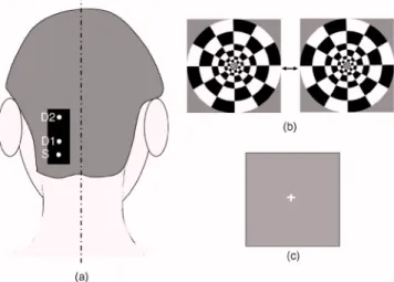
The lights from two diode lasers were combined using a bifurcated glass fiber bundle with a nominal 2.7-mm core diameter 共Fiberoptics Technology, prototype兲. Detector fibers were glass fiber bundles, also with 2.7-mm core diameter. The optical fiber bundles共optodes兲 were attached to a flexible piece of plastic that was attached to a black Velcro headband that fastened snugly around the head of the subject. Soft black Velcro was also used to absorb stray light beneath the probe. The combined light of two wavelengths were in contact with tissue in one source location关S in Fig. 1共a兲兴, and exiting light was collected from two detector locations,1.5 cm and 4.5 cm from the source, respectively关D1 and D2 in Fig. 1共a兲兴.
During the visual task, the multichannel NIRS probe was positioned 2 cm lateral and parallel to the subject’s midline, over the primary/secondary visual cortex 共confirmed by an existing MRI scan兲, with the source 1 cm inferior to the inion 关Fig. 1共a兲兴. MRI images also show that the thickness of the scalp and skull at this location is approximately2.1 cm, and with this probe configuration, photon propagation theory sug-gests that measurement from S-D1 will be sensitive to scalp and skull changes, while measurements from S-D2 will be sensitive to scalp, skull, CSF, vision cortex, and some white matter regions. The subject sat upright in a comfortable chair in a dark and quiet room facing a laptop screen. The stimulus consisted of a counterphased, 100% contrast radial checker-board 共5-Hz luminance reversals兲 covering approximately 20 deg of the visual field关Fig. 1共b兲兴. This was alternated with a mean-luminance, uniform field with a central fixation cross 关Fig. 1共c兲兴. One 8-min run of 16 blocks was presented, where each block consisted of checkerboard oscillation for15 s, fol-lowed by the fixation background for 15 s; thus, the base visual stimulation frequency was0.033 Hz.
2.2 Data Analysis
The raw 200-Hz optical data were offset-corrected and further digitally low-pass filtered, in addition to the instrument filter, using a 1.25-Hz, sixth-order Butterworth filter. The optical measurements for each channel were converted to relative changes in the concentration of HHb and O2Hb using the
modified Beer-Lambert law.38–41Concentration measurements were then bandpass filtered using a sixth-order Butterworth low-pass filter at 1.25 Hz in series with a sixth order Butter-worth high-pass filter at 0.004 Hz 共to remove any slowly drifting signal components兲 and then down-sampled to 20 Hz. Based on our previous Monte Carlo simulations with common head structure and tissue optical properties,36we chose DPFs of 5.4 and 7.0 for S-D1 and S-D2 at690 nm, and 5.1 and 6.6 for S-D1 and S-D2 at 830 nm. 共We initially set all DPFs to 6.0 for the data analysis, and the results closely mirrored the results reported here, suggesting insensitivity to DPF errors.36 The reported DPFs are based on more realistic Monte Carlo
Fig. 1 共a兲 Probe configuration for the vision test. 共b兲 Vision stimula-tion: alternating counter-phased radial checkerboard.共c兲 Rest period: uniform field with a central fixation cross.
estimates of DPF differences across wavelengths and separa-tions.兲 The time series of O2Hb concentration changes ac-quired from both source-detector pairs共S-D1 and S-D2兲 were fed into the adaptive filter. 共HHb was filtered similarly but separately.兲 The adaptive filter used a finite impulse response 共FIR兲 and transversal structure 共tapped delay line兲, with 100 nodes 共“weights”兲. The Widrow-Hoff least-mean-squared 共LMS兲 adaptation algorithm was used to optimize the filter coefficients on a sample-by-sample basis. The details can be found in our previous report.36The convergence control pa-rameter was = 0.0001. In order to speed the convergence, we prenormalized the target and the reference data sets by dividing by their estimated standard deviation so that both time series have a standard deviation of approximately 1. Af-ter the adaptive filAf-tering, the quantitative values of the filAf-tered results were recovered by multiplying back the standard de-viation. The initial guess of the adaptive filter weights was 关1 0 ...0兴—in other words, we assume that the shape of the global interference and the S-D1 measurements are identical at the beginning of the adaptive filtering. If this initial guess were to remain constant, it would be similar to Saager and Berger’s approach, which assumes that the entire S-D1 time series can be least-squares fit to and subtracted from the S-D2 measurement.35Our approach differs in that共1兲 we assume a linear mapping between S-D1 and S-D2 and that this mapping is dependent on recent history 共here, 100 weights instead of the entire time series, making the approach particularly suited to real-time applications兲, and 共2兲 that this mapping is allowed to change over time, which in principle allows us to handle nonstationary time series共see Sec. 4.2兲.
As in previous NIRS studies, we performed block ave-raging using nonoverlapping portions of the data set triggered on stimulus onsets 共averaging windows 2 s prior to checker-board onset and28 s after the onset of each block of visual stimulation兲.
After adaptive filtering, in order to retrieve the quantitative functional hemodynamic changes in the deep cortex layer in our previous Monte Carlo simulation study,36we calculated a sensitivity correction scaling factor. This is done by introduc-ing a known perturbation into the blood content of the simu-lated gray matter layer only and then calculating the blood content changes using the surface measurements and the MBLL. The sensitivity correction factor is defined as the ratio of true blood concentration change to measured blood volume change. In the simulation with general physiological param-eters, this sensitivity correction factor is calculated to be 27.5 forO2Hb and 26.4 for HHb, and we assumed the same
cor-rection factor in this human study.
Power spectral density 共PSD兲 was used to identify the components and vision stimulation–associated changes in the hemodynamic responses or other physiological signals. PSD was estimated inMATLAB共based on Welch’s averaged,
modi-fied periodogram method, with a Hanning window for smoothing兲. In order to find peaks that are statistically signifi-cant, we chose a confidence interval of 0.95 and calculated the upper and lower bound of the power spectrum within this interval. Usually, we say a peak can be identified if the lower bound of the peak is above the averaged surrounding noise floor shown in the PSD.
With PSD, we can also perform a quantitative CNR analy-sis. For human subject data, we cannot totally separate signal and noise. Thus, we roughly calculate the signal power by integrating the power共in linear scale兲 from the PSD over the “signal bands,” which are the small frequency segments sur-rounding the stimulation frequency and its second harmonic. This way, the evoked brain activity peak will normally be included. We integrate the rest of the power spectrum共“noise bands”兲 to get the noise power. The unavoidable error in this calculation includes real signal power in the noise band and actual noise power in the signal bands. The CNR is then cal-culated as the square root of the ratio of signal power to noise power. It is worth mentioning that since the PSD is calculated using the whole data set共9674 points at 20 Hz sampling rate, no overlap in the PSD segmentation兲, the CNR calculated based on this PSD is the result of averaging the whole data set, not the CNR for a single stimulation.
3 Results
3.1 Origins of Global Interference: Comparing
Optical, Respiration, and Cardiac Measurements
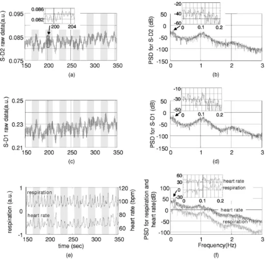
The respirometry and EKG were recorded simultaneously with optical measurements in order to help us determine the origins and understand the nature of the global interferences. The raw optical measurements共light intensity兲 at 830 nm col-lected from the “far” detector 共S-D2 with 4.5-cm source-detector separation兲 and from the “near” detector 共S-D1 with 1.5-cm source-detector separation兲 are shown in Figs. 2共a兲 and 2共c兲, respectively. In order to more clearly view the de-tails, such as the temporal correlation between different chan-nels, we have shown here only200 s of data. The associated power spectral densities are shown in Figs. 2共b兲 and 2共d兲. The simultaneously recorded respiration signal 共left y axis with arbitrary unit, indicating the movement of the upper abdo-men兲 and heart rate 共right y axis, calculated from the EKG兲 are presented in Fig. 2共e兲, and the associated PSD is shown in Fig. 2共f兲. The insets in Figs. 2共b兲, 2共d兲, and 2共f兲 show the details of PSD at frequencies less than0.2 Hz. Each PSD was estimated using all 96,736 data points so that more details can be seen at the low-frequency end. To avoid possible confu-sion, we need to point out again that the lower curve in Fig. 2共e兲 is the heart rate, not the EKG, and its spectrum in Fig. 2共f兲 is actually the spectrum for heart rate variation 共HRV兲.
In Figs. 2共a兲 and 2共c兲, we see that both optical measure-ments consist of a slow variation and a fast oscillation. The fast oscillation is obviously due to cardiac activity, it co-registers strictly with the EKG 共not shown兲, and the inset in Fig. 2共a兲 shows an enlarged data segment to demonstrate the temporal details of these fast signal fluctuations. The PSD of the optical signals, shown in Figs. 2共b兲 and 2共d兲, show that the cardiac activity peaks at 1.1 Hz, and its second harmonic at about2.2 Hz is also very obvious.
From the respiration PSD 关the inset in Fig. 2共f兲兴, we see that the principal respiration frequency is at 0.16 Hz. However, for both optical measurements 关seen in the insets in Figs. 2共b兲 and 2共d兲兴, the major low-frequency peak is ⬃0.1 Hz 共with a 0.16-Hz peak appearing about 10-dB down, and among peaks that might be artifacts兲. The heart rate PSD
关inset in Fig. 2共f兲兴 helps in explaining the origin of this 0.1-Hz peak in optical channels. The heart rate PSD shows 0.1 Hz and 0.16 Hz as the top two principal peaks, with the 0.1-Hz peak as the highest and 2 dB above the 0.16-Hz peak. 共The latter is obviously due to the respiratory sinus arrhyth-mia.兲 This suggests that the 0.1-Hz oscillation in the optical channels is physiological rather than artifact. Since0.1 Hz is the prototypical LFO frequency, we suspect that this oscilla-tion in the hemodynamics shown in the optical channels is vasomotor waves, and the0.1-Hz peak in the heart rate PSD is possibly an associated change in a vasomotor reflex. Full separation of component signals is difficult in this subject, because the subject’s respiration rate is relatively low, and we lack other more direct measurements such as invasive arterial pressure.
Optical measurements from far and near channels are very similar, actually a linear correlation analysis that shows that they are highly correlated 共r=0.91, p⬍10−20兲. The fact that the target 共far兲 measurement and reference 共near兲 measure-ment are highly correlated and that they all demonstrate major PSD peaks at heart beat and LFO frequencies indicates that the optical measurement from S-D2 is heavily contaminated
by global interference共measured by S-D1兲, as was previously derived via Monte Carlo experiments.
We performed a T-test on the 16 averaged heart rates dur-ing vision stimulation periods 共67.0±2.5 bpm兲 and the 16 averaged heart rates during rest periods共66.4±2.5 bpm兲. The change was not significant 关T共30兲=−0.7, p=0.24兴, suggest-ing no obvious heart rate increase or associated hemodynamic interference due to the visual stimulation itself.
To summarize, the PSD in the optical and physiological measurements suggests that the systemic interference comes from mixed sources, with cardiac activity and LFO 共Mayer waves or vasomotor waves, judging from the frequency兲 be-ing dominate. The visual stimulation does not cause any heart rate increase.
3.2 O2Hb Changes during Visual Stimulation
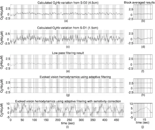
Changes in O2Hb during visual stimulation are shown in
Fig. 3. Here, Figs. 3共a兲 and 3共b兲 represent the target measure-ment of O2Hb calculated from the raw “far” signal and its
block average. Figures 3共c兲 and 3共d兲 show the reference O2Hb 共“near” signal兲 and its block average. Although the
Fig. 2 共a兲 The raw optical measurement at 830 nm from S-D2 with 4.5-cm source-detector separation 共the inset of an enlarged data segment shows
the heartbeats兲, and 共b兲 its power spectral density magnitude 共the inset shows the details at frequencies ⬍0.15 Hz兲. 共c兲 Raw optical measurement at 830 nm from S-D1 with 1.5-cm source-detector separation, and共d兲 its power spectral density magnitude. 共e兲 The top curve is the normalized voltage output from the respiration sensor, and the bottom curve is the heart rate in beats per minute共bpm兲, calculated from EKG recordings, and 共f兲 their power spectral density. The 1, 2, and 3 in 共a兲, 共c兲, and 共e兲 indicate the sequence of an example wave in respiration, heart rate, and optical.
target data set was expected to contain an increase in O2Hb following stimulus onset共and concomitant decrease following stimulus offset兲, neither the raw time series nor the block average show any obvious expected signal change. We hy-pothesized that the global interferences obscured the expected brain-relatedO2Hb change. The fact that the signal variations
in the targetO2Hb closely match those of the reference O2Hb
共which should contain no visual response兲 suggested that in-deed global interference may dominate the target data set.
The target data set after adaptive filtering is shown in Figs. 3共g兲–3共j兲. Figures 3共g兲 and 3共h兲 show the raw adaptive filtered result with its block average, and 3共i兲 and 3共j兲 show the filtered result following sensitivity correction. Comparing Figs. 3共g兲 and 3共h兲 关or their sensitivity-corrected versions in 3共i兲 and 3共j兲兴 with 3共a兲 and 3共b兲, we see that after adaptive filtering, both LFO and cardiac interference are substantially reduced 共actually, 80% of the signal variation was removed兲, while at the same time, the CNR of the hemodynamic re-sponses to vision stimulation increased dramatically. Both the time series’ and the block averaged results show an expected increase following stimulation onset and return to baseline during rest periods, with temporal changes appropriately as-sociated with the stimulation paradigm. For the detected vi-sual response shown in Fig. 3共j兲, we see a uniphase increase starting from approximately 2 s after stimulus onset, which plateaus at about9 s. The response remains steady until after the visual stimulation ends共we suspect that the hump at about 17 s is artifact兲, and begins to decrease at about 20 s,
recov-ering to baseline at about25 s. Although unlike in our previ-ous Monte Carlo simulation study, here we do not have a true O2Hb visual response value to compare with, the quantitative
O2Hb changes match previous reports.9,10
We also compared the adaptive filtering result with the traditional low-pass filtering result. O2Hb acquired from the
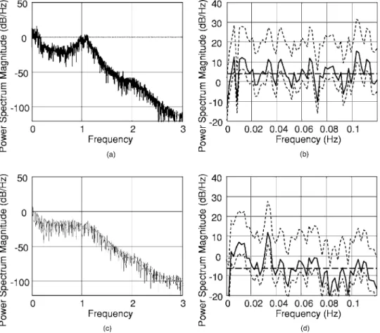
far detector 关S-D2, Fig. 3共a兲兴 is low-pass filtered with an eighth-order Butterworth filter with0.125 Hz bandwidth, and the result is shown in Figs. 3共e兲 and 3共f兲. From Fig. 3共e兲, we can see that this low-pass filter effectively removes the car-diac oscillations; however, systemic variations due to LFO remain. After block averaging, seen in Fig. 3共f兲, the systemic interference was further suppressed; however, it is still too large to reveal clear evoked brain activity. Comparing with the final adaptive filtering block averaged result关Fig. 3共j兲兴, we can see that adaptive filtering removes the global interference and recovers the evoked brain activity much more effectively. The CNR improvement from adaptive filtering can be quantitatively estimated using power spectral density tech-niques. Figure 4共a兲 shows the PSD of the target O2Hb before adaptive filtering, in which we see two dominating peaks at about1 Hz and 0.1 Hz, which correspond to cardiac activity and LFO. Figure 4共b兲 shows the details of the PSD of target O2Hb in 0 to 0.12-Hz range 共solid line兲, together with its
upper and lower bound calculated at a confidence interval of 0.95. In Fig. 4共b兲, using the average local noise level 共hori-zontal dashed line; averaged PSD magnitude in the 0 to
Fig. 3 Adaptive filtering to remove global interference and recover evoked brain activity.共a兲 Target O2Hb measurements from S-D2 with 4.5-cm source-detector separation, and共b兲 its block averaged result. 共c兲 and 共d兲 Reference measurements from S-D1 with 1.5-cm source-detector separa-tion.共e兲 and 共f兲 Low-pass filtering result for the target measurements. 共g兲 and 共h兲 Adaptive filtering result for the target measurement. 共i兲 and 共j兲 Adaptive filtering result with sensitivity correction.
0.12 Hz range兲 as the detection threshold 共to compare with the lower bound of the PSD兲, we can see several peaks above this threshold 共e.g., at 0.006 Hz, 0.012 Hz, 0.043 Hz, 0.066 Hz, 0.104 Hz, and 0.1 Hz兲, the LFO peak being the most significant one, about12 dB above. A peak of 0.033 Hz, the expected visual stimulation frequency, is actually among detected peaks; however, it is the second smallest compared with other detected peaks, only7 dB above the threshold, and difficult to distinguish among the other detectable peaks as real or artifact. After adaptive filtering关Fig. 4共c兲兴, the physi-ological interference due to LFO and cardiac activity peaks was significantly reduced. From the details presented in Fig. 4共d兲, we can see that the noise floor 共horizontal dashed line兲 was 10 dB less than the original, while the visual re-sponse peak remains 关compared with Fig. 4共b兲兴. Now only two peaks can be detected共0.010 Hz and 0.033 Hz兲, and the peak at 0.033 Hz, corresponding to vision stimulation, is the most significant peak and is18 dB above the local noise floor. If we choose the signal bands of the vision response to be roughly 0.028 to0.039 Hz共base band兲 and 0.061 to 0.072 Hz 共second harmonic兲, and the rest of the spectrum in the 0 to 10 Hz range is the noise bands, our CNR analysis shown that adaptive filtering doubled the CNR 共from 40.2% to 80.8%兲. The very low frequency of ⬃0.01 Hz was also preserved. It
remains to be determined whether signal variation at this fre-quency range is real or artifact.
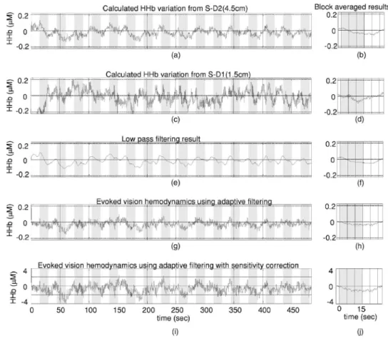
3.3 HHb Changes during Vision Stimulation
The adaptive filtering results for HHb are shown in Fig. 5. As for Figs. 3共i兲 and 3共j兲, Figs. 5共i兲 and 5共j兲 again utilized sensi-tivity correction. The PSD result is shown in Fig. 6.
One obvious difference in the HHb data as compared to O2Hb is that for HHb, the interference was relatively small
and the hemodynamic response was visible before adaptive filtering 关Figs. 5共a兲 and 5共b兲兴. In addition, the signal from the near detector 共shallow layer hemodynamics兲 differs more substantially from the far detector signal 共deep-layer hemodynamics兲—that is, the far detector HHb signal was not dominated by synchronized global interference. We suspect that interferences here have local origins and thus are different at different detector locations. This explanation is supported by the PSD analysis. In the PSD of target HHb measurement 关Figs. 6共a兲 and 6共b兲兴, we actually see no obvious LFO, respi-ration, or cardiac activity peaks. In other words, the major global interference sources in HHb are not significant. In Sec. 5, we discuss why in this subject HHb did not demonstrate obvious global interference peaks, as previously observed in O2Hb.
Fig. 4 共a兲 and 共b兲 present the power spectral density of O2Hb before adaptive filtering. 共a兲 is the PSD of O2Hb acquired from S-D2共4.5-cm source-detector separation兲 before adaptive filtering. 共b兲 shows the details of the PSD in the 0 to 0.12-Hz range. The solid line is the PSD magnitude, and the dotted line is the upper and lower bound calculated at a confidence interval of 0.95. The horizontal dashed line indi-cates the average noise level共averaged PSD magnitude in the 0 to 0.12-Hz range兲. 共c兲 and 共d兲 present the filtered result in the same way as 共a兲 and共b兲.
Since the amount of interference in the target data set is relatively small and the visual response and the global inter-ference are mostly independent of each other, the adap-tive filtering did not substantially alter the signal. As seen in Figs. 5共g兲 and 5共h兲, the overall amplitude of variations after adaptive filtering have only slightly changed 共17% smaller兲, unlike the O2Hb adaptive filtering results, where 80% of the
variations in the target data set were removed关Figs. 4共g兲 and 4共h兲兴. Comparing the results before and after adaptive filtering 关Figs. 5共a兲 with 5共g兲, respectively兴, we see that the visual response is clear in both, although adaptive filtering appears to slightly reduce the signal and increase noise. This can be more clearly seen in the PSD analysis in Figs. 5共b兲 and 5共d兲, where we see a 5.9-dB reduced peak at 0.033 Hz, and a 0.89-dB elevated noise level. The previous CNR analysis shows a 35% reduction of CNR after adaptive filtering.
When comparing Figs. 5共i兲 and 5共j兲 with the low-pass fil-tering result shown in Figs. 5共e兲 and 5共f兲 共which use an eighth-order Butterworth filter with0.125-Hz bandwidth兲, we can see that the low-pass filtering result is smoother. The shape of the response in 5共j兲 共onset, rise, offset, and fall times兲 has less low frequency fluctuation and is slightly more tem-porally consistent with prototypical hemodynamic responses than that in Fig. 5共f兲, but it is unclear if this is because of adaptive filtering.
For the filtered and sensitivity-corrected visual response shown in the block averaged and sensitivity corrected results in Fig. 5共j兲, we see a uniphase decrease starting from approxi-mately1 s after the onset of the stimuli, which continues until about8 s, when it reaches a valley. The signal remains at this value until after the visual stimulation ends, and it begins to increase at about 21 s, again recovering to baseline at about 25 s. These quantitative HHb changes due to vision stimula-tion also match those found in previous reports.9,10
The improvement from adaptive filtering on HHb in this case is not obvious. Although the shape of the filtered results 关Fig. 5共j兲兴 seems to agree more with expectations compared with Fig. 5共b兲 without adaptive filtering, it is unclear if this slight improvement is really from adaptive filtering, and the CNR estimated using PSD is actually reduced共from 66.5% to 43%兲. This suggests that in the cases where hemodynamic signals demonstrate obvious functional brain response and its PSD demonstrate no obvious global interference sources, adaptive filtering may be unnecessary.
4 Comparison of Shallow Layer Hemodynamics
and Estimated Global Interference
The performance of our method depends on whether the shal-low layer hemodynamics acquired from S-D1 and global
in-Fig. 5 Adaptive filtering to remove global interference and recover evoked brain activity.共a兲 Target HHb measurements from S-D2 with 4.5-cm
source-detector separation, and共b兲 its block averaged result. 共c兲 and 共d兲 Reference HHb measurements from S-D1 with 1.5-cm source-detector separation.共e兲 and 共f兲 Low-pass filtering result for the target measurements. 共g兲 and 共h兲 Adaptive filtering result for the target measurement. 共i兲 and 共j兲 Adaptive filtering result with sensitivity correction.
terference in the visual response detection acquired from S-D2 are correlated. When they are well correlated, the global interference can be optimally canceled, and the CNR of the evoked hemodynamic response is improved. A further ques-tion is whether the relaques-tionship is static or dynamic. Since it is difficult to precisely separate global interference from the raw S-D2 blood content time series, and since the visual response we acquired after adaptive filtering seems quite reasonable, we chose to estimate the global interference by subtracting the visual response关Fig. 3共g兲兴 from the raw time series with both interference and visual response embedded关Fig. 3共a兲兴 and use the residual as global interference. Although it is not math-ematically strict 共the “estimated global interference” is actu-ally the component in the target signal that correlates most with the reference signal, picked up by the adaptive filter兲, the fact that we subtract a decent visual response makes this es-timation acceptable, since generally the target signal is the combination of visual response and interference.
4.1 Stationary Comparison
In Fig. 7, we compare our two raw concentration time series directly by mean-subtraction and dividing each time series by its own 共temporal兲 standard deviation. Only a small segment is shown for clarity. Here, the normalizedO2Hb concentration
acquired from the near measurement 共S-D1兲 is shown as the dashed line and the computed O2Hb global interference
关Fig. 3共a兲 minus Fig. 3共g兲兴 is the solid line. As shown, the
two time series are highly overlapping. Actually, a linear re-gression of the two measurements 关Fig. 8共a兲兴 shows that the correlation coefficient between these two time series is 0.96 共p⬍10−20兲. Although the estimated global interference may
Fig. 6 共a兲 and 共b兲 present the power spectral density of HHb before adaptive filtering. 共a兲 is the PSD of HHb acquired from S-D2 共4.5-cm
source-detector separation兲. 共b兲 shows the details of the PSD in the 0 to 0.12-Hz range. The solid line is the PSD magnitude, and the dotted line is the upper and lower bound calculated at a confidence interval of 0.95. The horizontal dashed line indicates the average noise level共averaged PSD magnitude in the 0 to 0.12-Hz range兲. 共c兲 and 共d兲 present the filtered result in the same way as 共a兲 and 共b兲.
Fig. 7 Comparison of normalized shallow-layer hemodynamics
be different from real global interference, this correlation comparison demonstrates the similarity of the reference signal to the target signal after the visual response is removed and in turn explains why adaptive filtering removes the interference term very effectively.
4.2 Dynamic Comparison
Our previous analysis suggests that there is reasonably a lin-ear relationship between the shallow layer hemodynamics and global interference; however, this relationship changes with time. In Fig. 8共b兲, one segment of global interference is plot-ted against the shallow layer hemodynamics 共from 250 s to 270 s; both are smoothed using a sixth-order 0.25-Hz Butter-worth filter兲, and the arrow shows how the data moves with time. The data did not strictly follow the line. Thus, we per-formed short-term linear regressions—that is, we perper-formed linear fits using only 100 data points at a time共5 s兲 and slid the data window through the entire data set, with the esti-mated global interference as the independent time series and the near O2Hb measurement as the dependent variable. The
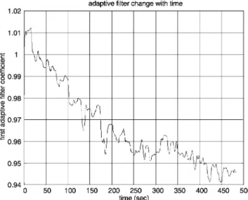
resulting linear fit slope and intercept values oscillate over time共Fig. 9兲. This dynamic feature can also be viewed in the adaptive filtering, where the node is adjusted at a point-by-point basis and is following the slow nonstationary variations of the time series to optimize the interference cancellation. The update of the first node as a function of time is presented in Fig. 10.
In this case study, the fact that the shallow layer hemody-namic changes correlated well with the global interference and that adaptive filtering in general follows the nonstationary changes in the time series explains why our method should work well in suppression of the global interference and im-prove the CNR in the evoked brain activity detection.
5 Discussion
This case study provides a preliminary demonstration of the potential effectiveness of our combined adaptive filter/ multidistance methodology for global interference reduction. From this study, we see the effect of adaptive filtering both in the situation when global interference dominates 共e.g., in O2Hb兲 and when the global interference does not dominate
Fig. 8 共a兲 Linear regression between the global interference in O2Hb from S-D2共vision response subtracted兲 and O2Hb from S-D1. 共b兲 A continuous plot of one 20-s segment. The arrow indicates the direction of change as a function of time.
Fig. 9 Short-term linear regression coefficients. The top curve is the
共e.g., in HHb兲. Clearly, adaptive filtering is substantially more useful in the former case. The key for adaptive filtering to work is that the interference must be common to both the signal channel and the reference channel. In principle, cardiac activity, respiration, and vasomotor waves should be common in the whole circulation system; however, because of the het-erogeneity of the vasculature in tissue and the location of the probe 共e.g., relative to large vessels兲, together with local changes at each optode, different optical measurements may be affected by different types of interference to a different degree, and not all optical measurements are dominated by the same type of interferences. To maximize the benefit of adap-tive filtering, one must first determine whether a given signal is substantially affected by global interference common to both the signal channel and the reference channel 共e.g., via PSD comparison兲. If the target channel shows interference similar to the reference channel, then apply the adaptive filter. Otherwise, skip adaptive filtering.
It was interesting to observe that HHb 共found mostly in venous compartments兲 exhibited little global interference, whereas the global interference inO2Hb共present in all
com-partments兲 was substantial. This makes sense in light of signal frequencies, which indicate that the interference was largely vasomotor or Mayer waves, which are arterial pressure waves.25 Since this is only a case report and the goal is to demonstrate the methodology, no physiological generaliza-tions should be drawn共N=1兲. For example, the subject in this case report showed an HHb response but not an O2Hb
re-sponse after block averaging. We believe this occurred be-cause of excessive physiological interference of the overlying layers and predominantly inO2Hb, a problem which was
sub-stantially resolved by adaptive filtering. In other studies, group averages normally show O2Hb and HHb responses,
with a certain amount of variability. Results from individual subjects, however, are even more variable, sometimes show-ing clear responses in both O2Hb and HHb, sometimes only
in one Hb species, and sometimes in neither.
The sensitivity correction factor is a constant that converts the evoked brain hemodynamics acquired from surface mea-surements and MBLL to quantitative blood content changes in the cortex. Based on the photon transport theory, this con-stant changes with parameters such as the probe configuration and dimensions and the optical properties of different layers of the head. Since not all this information is known in our test, errors in the assumed sensitivity correction number in our study are unavoidable. However, since the focus of our study is to demonstrate the effectiveness of adaptive filtering by looking at the contrast-to-noise changes, and this constant changes the quantitative results of the关HHb兴 and 关O2Hb兴 but
not the CNR共this sensitivity correction factor is canceled in the CNR calculation兲, the conclusions of this case study should not be affected by the error in the sensitivity correction factor.
The overall performance of this adaptive filtering approach to removing global interference during in vivo applications depends on whether the shallow layer hemodynamics provide a good estimate of the global interference in the target data set. According to photon transport theory, optical measure-ments are more sensitive to superficial layers, and we have demonstrated using Monte Carlo simulation that
hemody-namic changes in the superficial layers is the major compo-nent of the global interference in evoked brain activity detec-tion. Furthermore, since the blood vessels for the superficial and deep layers are connected and can be closely traced back to the same origin, namely, the common carotid arteries, one might expect hemodynamics in these layers to be reasonably correlated. Thus, it would seem to be a reasonably general principle that the scalp and skull hemodynamics acquired us-ing optical measurements with short source-detector separa-tion should provide a good estimate of the global interference in measurements of deeper layers. The observed correspon-dence between shallow layer hemodynamics and global inter-ference in this case study explains why this can work on hu-man subjects when global interference dominates.
In addition, since living human tissue is a very nonstation-ary system, we expect the relationship between the shallow layer hemodynamics and the global interference to change with time, as observed in this case. The adaptive filtering method assumes that there exists a linear mapping between the reference and the target data set. This mapping is allowed to change, but the change needs to be “slow enough” for adaptive filtering to follow. This slowness depends on the convergence of the adaptive filtering method and the magni-tude of the mapping change. We chose one of the simplest available adaptive filtering methods and parameter optimiza-tion approaches 共LMS兲. Many other methods could be ap-plied, with better convergence rates, while maintaining good stability and robustness. These approaches remain to be ex-plored, as here we sought only to demonstrate the suitability of the approach for real physiological data.
In many applications, it is desirable to have interferences removed in real time. In some applications, including func-tional brain area localization and biofeedback, this real-time feature is mandatory. The adaptive filtering method we used is computationally trivial and hence can be easily implemented in real-time manner. Based on the extensive knowledge base surrounding adaptive filtering techniques, several techniques can help improve the convergence of the adaptive filter. First, since the convergence and stability of the LMS algorithm de-pends on the energy of input signals, normalization 共so that both target time series and reference time series have roughly a standard deviation of one兲 increases the convergence rate and standardization of the choice of initial value of the adap-tive filter and the step control parameter. Second, a pretest is needed to train the adaptive filter before the real brain activity detection can be utilized to generate a better initial guess at node weights. From the pretest, we can estimate the amplitude of the target measurement and reference measurement, and these values can be used in the normalization of the two time series. It would also allow the adaptive filter to reach a rea-sonable value, to be used as the initial filter coefficient for the real test. When really high filtering speed is required, such as in some real-time imaging of brain activity, one may even consider the normalization-subtraction method described in a previous report共Sec. 2, Eq. 共5兲 in Ref. 36兲, where the amount of calculation is minimized.
In Fig. 3, before filtering, the quantitative amplitude of the concentration changes at the far separation 关Figs. 3共a兲 and 3共b兲, from S-D2兴 is only about half of that acquired from the near separation关Figs. 3共c兲 and 3共d兲, from S-D1兴. This might be due to a partial volume effect and suggests that the spatial
origins of the major physiological variations may be limited to a thin, vascularized layer共e.g., the dermis layer of skin兲. As the sampling volume photon probes increase with source-detector separation, the percentage of area with hemodynamic variation over the whole sampling volume decreases, and thus the amount ofO2Hb variations acquired using MBLL is re-duced. In principle, one could compensate for such a layer using sensitivity correction, although this would require knowledge of the location and thickness of that vascularized layer. The result in Fig. 3 also indicates that in our experi-ment, a direct subtraction of reference signal关Fig. 3共c兲兴 from the target signal关Fig. 3共a兲兴 will not work for the purpose of removal of global interference, because quantitatively they are not comparable 共due to the difference in the average blood concentration in different tissue area, or partial volume ef-fect兲, and actually in our case, such subtraction will generate a negative result since S-D1 detects a much largerO2Hb
varia-tion than S-D2.
The fact that our adaptive filtering dramatically removes global interference and improves CNR inO2Hb in the evoked
brain hemodynamic response detection is exciting, and PSD analysis should be practical in helping to judge whether the optical measurements are global interference–dominated and adaptive filtering should be applied. However, the approach needs to be tested in different experimental settings and on larger sample sizes to assess the breadth of the method utility. For example, in this case study, the global interference and the evoked brain activity are not correlated 共suggested by the T-test of heart rates at the rest and stimulation periods兲, and further study is need to explore the results in the situation when the two are partly correlated. The case study described in this paper sets the data analysis platform for future human subject tests.
Acknowledgments
This work was supported by the NIH 共Grant Nos. K25-NS46554, R21-EB02416, R01-DA015644, and R01-EB006589兲. We would also like to thank Margaret Duff for her help preparing the manuscript.
References
1. B. Chance, “Optical method,” Annu. Rev. Biophys. Biophys. Chem.
20, 1–28共1991兲.
2. E. Gratton, V. Toronov, U. Wolf, M. Wolf, and A. Webb, “Measure-ment of brain activity by near-infrared light,” J. Biomed. Opt. 10共1兲, 011008共2005兲.
3. A. Yodh and B. Chance, “Spectroscopy and imaging with diffusing light,” Phys. Today 48共3兲, 34–40 共1995兲.
4. H. Obrig and A. Villringer, “Beyond the visible—imaging the human brain with light,” Kyklos 23共1兲, 1–18 共2003兲.
5. R. L. Barbour, H. L. Graber, Y. L. Pei, S. Zhong, and C. H. Schmitz, “Optical tomographic imaging of dynamic features of dense-scattering media,” J. Opt. Soc. Am. A 18共12兲, 3018–3036 共2001兲. 6. D. A. Boas, M. A. Franceschini, A. K. Dunn, and G. Strangman,
“Non-invasive imaging of cerebral activation with diffuse optical to-mography,” in: Optical Imaging of Brain Function, Frostig, R., Ed., CRC Press共2002兲.
7. A. Villringer, J. Planck, C. Hock, L. Schleinkofer, and U. Dirnagl, “Near-infrared spectroscopy 共NIRS兲—a new tool to study hemodynamic-changes during activation of brain-function in human adults,” Neurosci. Lett. 154共1–2兲, 101–104 共1993兲.
8. J. H. Meek, C. E. Elwell, M. J. Khan, J. Romaya, J. S. Wyatt, D. T. Delpy, and S. Zeki, “Regional changes in cerebral haemodynamics as a result of a visual stimulus measured by near infrared spectros-copy,” Proc. R. Soc. London, Ser. B 261, 351–356共1995兲.
9. P. Wobst, R. Wenzel, M. Kohl, H. Obrig, and A. Villringer, “Linear aspects of changes in deoxygenated hemoglobin concentration and cytochrome oxidase oxidation during brain activation,” Neuroimage
13, 520–530共2001兲.
10. M. L. Schroeter, M. M. Bucheler, K. Muller, K. Uludag, H. Obrig, G. Lohmann, M. Tittgemeyer, A. Villringer, and D. Y. von Cramon, “Towards a standard analysis for functional near-infrared imaging,”
Neuroimage, 21共1兲, 283–290 共2004兲.
11. H. Obrig, C. Hirth, J. G. Junge-Hulsing, C. Doge, T. Wolf, U. Dirnagl, and A. Villringer, “Cerebral oxygenation changes in re-sponse to motor stimulation,” J. Appl. Physiol. 81共3兲, 1174–1183 共1996兲.
12. V. Toronov, A. Webb, J. H. Choi, M. Wolf, A. Michalos, E. Gratton et al., “Investigation of human brain hemodynamics by simultaneous near-infrared spectroscopy and functional magnetic resonance imag-ing,” Med. Phys. 28共4兲, 521–527 共2001兲.
13. G. Jasdzewski, G. Strangman, J. Wagner, K. K. Kwong, R. A. Poldrack, and D. A. Boas, “Differences in the hemodynamic response to event-related motor and visual paradigms as measured by near-infrared spectroscopy,” Neuroimage 20共1兲, 479–488 共2003兲. 14. G. Strangman, J. P. Culver, J. H. Thompson, and D. A. Boas, “A
quantitative comparison of simultaneous BOLD fMRI and NIRS re-cordings during functional brain activation,” Neuroimage 17共2兲, 719– 731共2002兲.
15. C. Hock, K. Villringer, F. Muller-Spahn, R. Wenzel, H. Heekeren, S. Schuh-Hofer, M. Hofmann, S. Minoshima, M. Schwaiger, U. Dirnagl, and A. Villringer, “Decrease in parietal cerebral hemoglobin oxygenation during performance of a verbal fluency task in patients with Alzheimer’s disease monitored by means of near-infrared spec-troscopy共NIRS兲–correlation with simultaneous rCBF-PET measure-ments,” Brain Res. 755共2兲, 293–303 共1997兲.
16. M. A. Franceschini, S. Fantini, J. H. Thomspon, J. P. Culver, and D. A. Boas, “Hemodynamic evoked response of the sensorimotor cortex measured noninvasively with near-infrared optical imaging,”
Psycho-physiology 40共4兲, 548–560 共2003兲.
17. A. Watanabe and T. Kato, “Cerebrovascular response to cognitive tasks in patients with schizophrenia measured by near-infrared spec-troscopy,” Schizophr Bull. 30共2兲, 435–444 共2004兲.
18. A. Watanabe, K. Matsuo, N. Kato, and T. Kato, “Cerebrovascular response to cognitive tasks and hyperventilation measured by multi-channel near-infrared spectroscopy,” J. Neuropsychiatry Clin.
Neuro-sci. 15共4兲, 442–449 共2003兲.
19. G. Morren, M. Wolf, P. Lemmerling, U. Wolf, J. H. Choi, E. Gratton, L. De Lathauwer, and S. Van Huffel, “Detection of fast neuronal signals in the motor cortex from functional near infrared spectros-copy measurements using independent component analysis,” Med.
Biol. Eng. Comput. 42共1兲, 92–99 共2004兲.
20. M. A. Franceschini and D. A. Boas, “Noninvasive measurement of neuronal activity with near-infrared optical imaging,” Neuroimage
21共1兲, 372–386 共2004兲.
21. J. Steinbrink, F. C. D. Kempf, A. Villringer, and H. Obrig, “The fast optical signal-robust or elusive when noninvasively measured in the human adult?,” Neuroimage 26共4兲, 996–1008 共2005兲.
22. P. W. McCormick, M. Stewart, M. G. Goetting, M. Dujovny, G. Lewis, and J. I. Ausman, “Noninvasive cerebral optical spectroscopy for monitoring cerebral oxygen delivery and hemodynamics,” Clin.
Crit. Care Med. 19共1兲, 89–97 共1991兲.
23. P. W. McCormick, M. Stewart, G. Lewis, M. Dujovny, and J. I. Ausman, “Intracerebral penetration of infrared light,” J. Neurosurg.
76共2兲, 315–318 共1992兲.
24. M. Kohl-Bareis, H. Obrig, K. Steinbrink, K. Malak, K. Uludag, and A. Villringer, “Noninvasive monitoring of cerebral blood flow by a dye bolus method: separation of brain from skin and skull signals,” J.
Biomed. Opt. 7共3兲, 464–470 共2002兲.
25. A. C. Guyton and J. E. Hall, Textbook of Medical Physiology, Saun-ders共2005兲.
26. M. A. Franceschini, D. A. Boas, A. Zourabian, S. G. Diamond, S. Nadgir, D. W. Lin, J. B. Moore, and S. Fantini, “Near-infrared spiroximetry: noninvasive measurements of venous saturation in pig-lets and human subjects,” J. Appl. Physiol. 92共1兲, 372–384 共2002兲. 27. M. Manoach, S. Gitter, I. M. Levinger, and S. Stricker, “On the
origin of respiratory waves in circulation,” Eur. J. Physiol. 325共1兲, 40–60共1971兲.
28. G. I. Kositskii, “Respiratory waves of blood pressure in human sub-jects,” Bull. Exp. Biol. Med. 45共2兲, 154–157 共1958兲.
29. M. B. Visscher, A. Rupp, and F. H. Scott, “The respiratory wave in arterial blood pressure,” Am. J. Physiol. 70共3兲, 586–606 共1924兲. 30. H. Obrig, M. Neufang, R. Wenzel, M. Kohl, J. Steinbrink, K.
Einhaupl, and A. Villringer,, “Spontaneous low frequency oscilla-tions of cerebral hemodynamics and metabolism in human adults,”
Neuroimage 12共6兲, 623–639 共2000兲.
31. G. Gratton and P. M. Corballis, “Removing the heart from the brain: compensation for the pulse artifact in the photon migration signal,”
Psychophysiology 32共3兲, 292–299 共1995兲.
32. V. Kolehmainen, S. Prince, S. R. Arridge, and J. P. Kaipio, “State-estimation approach to the nonstationary optical tomography prob-lem,” J. Opt. Soc. Am. A 20共5兲, 876–879 共2003兲.
33. S. Prince, V. Kolehmainen, J. P. Kaipio, M. A. Franceschini, D. Boas, and S. R. Arridge, “Time-series estimation of biological factors in optical diffusion tomography,” Phys. Med. Biol. 48共11兲, 1491–1504 共2003兲.
34. Y. H. Zhang, D. H. Brooks, M. A. Franceschini, and D. A. Boas, “Eigenvector-based spatial filtering for reduction of physiological interference in diffuse optical imaging,” J. Biomed. Opt. 10共1兲 共2005兲.
35. R. B. Saager and A. J. Berger, “Direct characterization and removal of interfering absorption trends in two-layer turbid media,” J. Opt.
Soc. Am. A 22共9兲, 1874–1882 共2005兲.
36. Q. Zhang, E. N. Brown, and G. E. Strangman, “Adaptive filtering to removal global interference in evoked brain activity detection: a human subject case study,” J. Biomed. Opt. 12共4兲, 044014 共2006兲. 37. A. M. Siegel, J. J. A. Marota, and D. A. Boas, “Design and evaluation of a continuous-wave diffuse optical tomography system,” Opt.
Ex-press 4, 287–298共1999兲.
38. D. A. Boas, T. Gaudette, G. Strangman, X. Cheng, J. J. A. Marota, and J. B. Mandeville, “The accuracy of near infrared spectroscopy and imaging during focal changes in cerebral hemodynamics,”
Neu-roimage 13, 76–90共2001兲.
39. G. Strangman, M. A. Franceschini, and D. A. Boas, “Factors affect-ing the accuracy of near-infrared spectroscopy concentration calcula-tions for focal changes in oxygenation parameters,” Neuroimage
18共4兲, 865–879 共2003兲.
40. D. T. Delpy, M. Cope, and P. van der Zee, “Estimation of optical pathlength through tissue from direct time of flight measurement,”
Phys. Med. Biol. 33, 1433–1442共1988兲.
41. A. Villringer and B. Chance, “Non-invasive optical spectroscopy and imaging of human brain function,” Trends Neurosci. 20共10兲, 435–442 共1997兲.