HAL Id: hal-01918738
https://hal.archives-ouvertes.fr/hal-01918738
Submitted on 11 Nov 2018
HAL is a multi-disciplinary open access
archive for the deposit and dissemination of
sci-entific research documents, whether they are
pub-lished or not. The documents may come from
teaching and research institutions in France or
abroad, or from public or private research centers.
L’archive ouverte pluridisciplinaire HAL, est
destinée au dépôt et à la diffusion de documents
scientifiques de niveau recherche, publiés ou non,
émanant des établissements d’enseignement et de
recherche français ou étrangers, des laboratoires
publics ou privés.
A distributed and parallel unite and conquer method to
solve sequences of non-Hermitian linear systems
Xinzhe Wu, Serge Petiton
To cite this version:
Xinzhe Wu, Serge Petiton. A distributed and parallel unite and conquer method to solve sequences
of non-Hermitian linear systems. Japan Journal of Industrial and Applied Mathematics, Kinokuniya
Company, In press, �10.1007/s13160-019-00359-1�. �hal-01918738�
(will be inserted by the editor)
A Distributed and Parallel Unite and Conquer Method to
Solve Sequences of Non-Hermitian Linear Systems
Xinzhe Wu · Serge G. Petiton
Received: date / Accepted: date
Abstract Many problems in science and engineering often require to solve a long sequence of large-scale non-Hermitian linear systems with different Right-hand sides (RHSs) but a unique operator. Efficiently solving such problems on extreme-scale platforms requires the minimization of global communications, reduction of synchronization and promotion of asynchronous communications. Unite and Conquer GMRES/LS-ERAM (UCGLE) method [30] is a suitable candidate with the reduction of global communications and the synchro-nization points of all computing units. It consists of three computing algorithms with asyn-chronous communications that allow the use of approximate eigenvalues to accelerate the convergence of solving linear systems and to improve the fault tolerance. In this paper, we extend both the mathematical model and the implementation of UCGLE method to adapt to solve sequences of linear systems. The eigenvalues obtained in solving previous linear systems by UCGLE can be recycled, improved on the fly and applied to construct a new ini-tial guess vector for subsequent linear systems, which can achieve a continuous acceleration to solve linear systems in sequence. Numerical experiments using different test matrices to solve sequences of linear systems on supercomputer Tianhe-2 indicate a substantial decrease in both computation time and iteration steps when the approximate eigenvalues are recycled to generate the initial guess vectors.
Keywords Sequence of linear systems · Linear solvers · Krylov methods · Unite and Conquer · Iterative methods · Eigenvalues
Mathematics Subject Classification (2000) 00A69 · 65F10
This work is funded by the project MYX of French National Research Agency (ANR) (Grant No. ANR-15-SPPE-003) under the SPPEXA framework.
Xinzhe Wu ( )
[email protected] Serge G. Petiton
Maison de la Simulation, Gif-sur-Yvette Cedex, 91191, France
1 Introduction
We consider solving a long sequence of sparse and non-Hermitian linear systems
Ax= bi, i = 1, 2, 3, · · · (1)
where A ∈ Cn×n keeps the same, and bi∈ Cn changing from one system to another.
Moreover, these systems are typically not available simultaneously. This kind of linear sys-tems arise from a variety of applications in different scientific and engineering fields, such as the finite element analysis in modeling fatigue [14], diffuse optical tomography [19] and electromagnetic [32], etc. These systems are formatted either by the time-dependent appli-cations where the operator A remains the same, but bicannot be obtained simultaneously or
by the application of Newton methods for solving nonlinear systems (e.g., [4, 6, 12, 20]). Different techniques can be applied to reduce the time cost of solving subsequent sys-tems in sequence. If the direct solvers are appropriate, their factorizations can be shared and reused to solve continuous linear systems by forward/backward. If the matrix is sparse with a high dimension, and the direct solvers are not applicable, the iterative methods based on Krylov subspace, such as CG (Conjugate Gradient) method [18] for symmetric systems, and GMRES (Generalized minimal residual) method [26] for non-Hermitian systems, should be considered. In order to accelerate the convergence, the preconditioners can also be applied. For the linear systems with simultaneous RHSs, the block Krylov methods [3, 7, 15, 27] are applicable. For linear systems in sequence with different RHSs, since they share the same operator matrix A, the intermediate information computed from the procedures of solving previous systems can be reused to speed up the solves of subsequent systems. The seed ap-proach [1, 8, 13, 21, 24, 27, 28] selects one seed system and solves it by the Krylov iterative methods. Then, the optimal norm or orthogonality criterion on the Krylov subspace gener-ated by the seed system can be used to form the initial guess vectors of other linear systems. The seed method requires the extra memory space to store the subspace of seed systems, and its speed up cannot always be guaranteed for the uncorrelated right-hand sides. Another alternative is to recycle the Krylov subspace spectral information [5, 17, 19, 22, 32]. The most well-known method GCRO-DR (Generalized Conjugate Residual method with inner Orthogonalization and Deflated Restarting) proposed by Parks et al. [22] allows speeding up the procedure of solving systems from one RHS to another or even between two times restart of iterative methods through the maintenance of the Arnoldi subspace orthogonalization and the deflation of smallest eigenvalues by recycling the approximate invariant subspaces gen-erated by previous solving of linear systems.
However, nowadays, HPC cluster systems continue to scale up not only the number of compute nodes and central processing unit (CPU) cores but also the heterogeneity of com-ponents by introducing graphics processing units (GPUs) and manycore processors. This re-sults in the tendency of transition to multi- and many cores within computing nodes, which communicate explicitly through faster interconnection networks. These hierarchical super-computers can be seen as the intersection of distributed and parallel computing. Indeed, for a large number of cores, the communication of overall reduction operations and global synchronization are the bottleneck [9]. Consequently, large scalar products, overall synchro-nization, and other operations involving communication among all cores have to be avoided. The numerical methods should be adjusted to reduce the global synchronization points and promote asynchronization to adapt to multi-grain, multi-level memory with high fault tol-erance. The special process, e.g., the image projection and sparse matrix-vector product of seed methods, the external solving of eigenvalue problem and reduced QR decomposition
inside GCRO-DR introduce much more additional synchronization points across all cores. These operations damage the performance on extreme-scale platforms. Novel models of algorithms should be proposed to solve linear systems in sequence on large-scale platforms. UCGLE is a suitable candidate to solve linear systems with single RHS on extreme-scale supercomputing platforms, minimizing global communications and overall synchronization points. Its idea comes from the unite and conquer approach introduced by Emad [10] in 2016, which aims at exploring the novel methods for modern computer architectures. It is a model for the design of numerical methods by combining different computing components with asynchronous communication. Moreover, these components work for a same objective. In the unite and conquer methods, different parallel computing components work indepen-dently, which can be deployed on various platforms such as P2P, cloud, and the supercom-puter systems, or different computing units on the same platform. However, UCGLE that we talked about in this paper is only an implementation of unite and conquer approach targeting at the modern supercomputing platforms. UCGLE is a hybrid method which consists of three computing components with asynchronous communications: ERAM (Explicitly Restarted Arnoldi Method), GMRES and LS (Least Squares) components. GMRES Component is used to solve the systems, and LS Component performs as a preconditioner using the eigen-values approximated by ERAM Component to speed up the convergence. LS Component is implemented based on the Least Squares polynomial method proposed by Saad [23]. Com-pared with the classical hybrid methods using LS polynomial [11, 16, 33], the key features of UCGLE are its distributed and parallel asynchronous communications and the manager engine implementation among three components, specified for supercomputing platforms. Its asynchronous communications cover overall synchronization overhead and improve the fault tolerance. Better convergence acceleration and parallel performance of UCGLE using test matrices compared with preconditioned GMRES are given in [30].
Despite the advantages of UCGLE for large-scale platforms, it is not able to solve se-quences of linear systems with continuous improvement through the maintenance of in-termediate information. In this paper, we develop a variant of UCGLE to solve the linear systems in sequence by recycling the dominant eigenvalues. Indeed, when solving linear systems with UCGLE, more eigenvalues are approximated, and the more accurate they are, the more significant the acceleration. The eigenvalues obtained from the solves of previous systems can be reused and improved on the fly, to speed up the solves of successive systems. More importantly, these previously calculated eigenvalues can be applied to construct a new initial guess for current system using the LS polynomial method, and its convergence can be significantly accelerated. In this paper, we assume that the matrix A keeps the same for linear systems in sequence, but UCGLE is applicable even part of their spectra change slowly.
The paper is organized as follows. In Section 2, we summarize the theory of numerical algorithms inside UCGLE, especially the LS polynomial method proposed by Saad. The introduction of LS polynomial method shows the fundamentals of recycling the eigenvalues. The extended implementation of UCGLE for solving sequences of linear systems is shown in Section 3. In Section 4, various experiments using UCGLE to solve linear systems in the sequence are presented. We give the conclusions and perspectives in Section 5.
2 UCGLE: Algorithms of Components
In order to give a glance at UCGLE, especially the way to recycle the eigenvalues to solve sequences of linear systems, we summarize the mathematical models and algorithms of three components inside UCGLE in this section.
GMRES and ERAM algorithms inside UCGLE are both Krylov subspace methods. In linear algebra, the m-order Krylov subspace generated by a n × n matrix A and a vector b of dimension n is the linear subspace spanned as:
Km(A, b) = span(b, Ab, A2b, · · · , Am−1b) (2)
Arnoldi reduction is able to build an orthogonal basis of Km. As shown in Algorithm 1, at
each step of Arnoldi reduction, it multiplies the previous Arnoldi vector νjby matrix A, and
get an orthogonal vector νj+1 against all previous ωiby a stand Gram-Schmit procedure.
It will stop if the vector computed in line 7 is zero. The vectors ω1, ω2. · · · , ωmform an
orthonormal basis of the Krylov subspace.
Algorithm 1 Arnoldi Reduction
1: function AR(input:A, m, ν, out put: Hm,Vm)
2: ν1= ν/||ν||2 3: for j = 1, 2, · · · , m do 4: hi, j= (Aνj, νi), for i = 1, 2, · · · , j 5: ωj= Aνj− ∑i=1j hi, jνi 6: hj+1, j= ||ωj||2 7: if hj+1, j= 0 then Stop 8: end if 9: νj+1= ωj/hj+1, j 10: end for 11: end function
Denote by Vm, the n × m matrix with column vectors ν1, ν2. · · · , νm, by Hm, the (m + 1) ×
mHessemberg matrix whose nonzero entries hi, jare defined by Algorithm 1, then note Hm
as the matrix obtained from Hmby deleting its last row. The following relations are given:
VmTAVm= Hm. (3)
In case that the norm of ωjin line 7 of Algorithm 1 vanishes at a certain step j, Hmturns
to be Hj with dimension j × j. The ERAM and GMRES components of UCGLE are both
the iterative methods based on the Arnoldi reduction.
2.1 ERAM Algorithm
The mission of ERAM Component inside UCGLE is to approximate the dominant eigenval-ues using ERAM, which is a variant of Arnoldi algorithm [2]. Arnoldi method is widely used to compute the eigenvalues of large sparse non-Hermitian matrices. Its kernel is the Arnoldi reduction, which gives an orthonormal basis Vm= (ν1, ν2, · · · , νm) of Km(A, ν), where A is
n× n matrix, and ν is a n-dimensional vector. With the relation (3), the eigenvalues of Hm
are the approximated ones of A, which are called the Ritz values of A. The r desired Ritz values Λr= (λ1, λ2, · · · , λr) can be gotten by basic Arnoldi method.
The numerical accuracy of the computed eigenpairs by basic Arnoldi method depends highly on the size of Km(A, v) and the orthogonality of Vm. Generally, the larger the subspace
is, the better the eigenpairs approximation is. The problem is that firstly the orthogonality of the computed Vmtends to degrade with each basis extension. Also, the larger the subspace
size, and so the achievable accuracy of the Arnoldi process. To overcome this, Saad [25] proposed to restart the Arnoldi process, which is the ERAM. The Krylov subspace size of ERAM is fixed as m, and only the starting vector will vary. After one restart of the Arnoldi process, the starting vector will be initialized using information from the computed Ritz vectors. Then the vector will be forced to be in the desired invariant subspace. The Algorithm
of ERAM is given by Algorithm 2, where εa is a tolerance value, r is desired eigenvalues
number and the function g defines the stopping criterion of iterations.
Algorithm 2 Explicitly Restarted Arnoldi Method
1: function ERAM(input: A, r, m, ν, εa, out put: Λr)
2: Compute an AR(input:A, m, ν, out put: Hm,Vm)
3: Compute r desired eigenvalues λi(i ∈ [1, r]) of Hm
4: Set ui= Vmyi, for i = 1, 2, · · · , r, the Ritz vectors
5: Compute Rr= (ρ1. · · · , ρr) with ρi= ||λiui− Aui||2
6: if g(ρi) < εa(i ∈ [1, r]) then
7: stop 8: else
9: set v = ∑di=1Re(νi), and GOTO 2
10: end if 11: end function
2.2 GMRES Algorithm
GMRES is a Krylov iterative method to solve non-Hermitian linear systems Ax = b. It ap-proximates the solution xmfrom an initial guess x0, with the minimal residual in a selected
Krylov subspace. It was introduced by Saad and Schultz in 1986 [26].
Algorithm 3 Basic GMRES method
1: function BASICGMRES(input: A, m, x0, b, out put: xm)
2: r0= b − Ax0, β = ||r0||2, and ν1= r0/β
3: Compute an AR(input:A, m, ν1, out put: Hm,Vm)
4: Compute ymwhich minimizes ||β e1− Hmy||2
5: xm= x0+Vmym
6: end function
In fact, any vector x in subspace x0+ Kmcan be written as
x= x0+Vmy. (4)
with y an m-vector, Ωman orthonormal basis of the Krylov subspace Km. The norm of
residual R(y) of Ax = b is given as:
R(y) = ||b − Ax||2= ||b − A(x0+Vmy)||2
= ||VM+1(β ei− Hmy)||2= ||β ei− Hmy||2.
(5) xmcan be obtained as xm= x0+Vmymwhere ym= argminy||β ei−Hmy||2. The minimizer
is the basic GMRES method as Algorithm 3. If m is large, GMRES can be restarted after a number of iterations, to avoid large memory and computational requirements with the increase of Krylov subspace projection number. The difficulty of restarted GMRES is that it can stagnate when the matrix is not positive definite. Usually, the preconditioning techniques or the deflation of eigenpairs are used to speed up the converge.
2.3 Least Squares Polynomial Algorithm
LS polynomial method is an iterative method proposed by Saad [23] in 1987 to solve linear systems. In this paper, it aims to calculate a new preconditioned residual for the restart of GMRES and to generate the initial guess vectors for solving the sequences of linear systems. 2.3.1 Polynomial Iterative Method
The iterates of LS polynomial method can be written as
xd= x0+ Pd(A)r0. (6)
where x0is an initial approximation of solution, r0the corresponding residual norm, and Pd
a polynomial of degree d − 1. We set a polynomial Rdof degree d such that
Rd(λ ) = 1 − λ Pd(λ ). (7)
The residual of dthsteps iteration rdcan be expressed as equation
rd= Rd(A)r0. (8)
with the constraint Rd(0) = 1. We want to find a kind of polynomial which can minimize
||Rd(A)r0||2, with ||.||2the Euclidean norm.
If A is a n × n diagonalizable matrix with its spectrum denoted as σ (A) = λ1, · · · , λn, and
the associated eigenvectors u1, · · · , un. Expanding the initial residual vector r0in the basis
of these eigenvectors as r0= n
∑
i=1 ρiui (9)and then the residual vector rdcan be expanded in this basis of eigenvectors as
rd= n
∑
i=1Rd(λi)ρiui (10)
which allows getting the upper limit of ||rd|| as
||rd||2≤ ||r0||2 max λ ∈σ (A)
|Rd(λ )| (11)
In order to minimize the norm of rd, it is possible to find a polynomial Pd which can
minimize the Equation (11). And it tends to be a minimum-maximum problem with the constraint Rd(0) = 1 and λ ∈ σ (A)
In the practical situation, when solving the linear systems by Least Squares Method, the whole number of eigenvalues λiof A are usually not available. But a region H in the real
complex plane that includes λ (A) can be constructed by the approximative eigenvalues of
A, and then the problem becomes as below with Rd(0) = 1
min maxλ ∈H|Rd(λ )| (13)
2.3.2 Least Squares Polynomial Preconditioning
Indeed, it is not always easy to approximate all the eigenvalues of A. Suppose that the total number of eigenvalues σ (A) can be divided into σk(A) = λ1, · · · .λk and σn−k(A) =
λk+1, · · · , λn, where σk are the first k known dominant eigenvalues, and σn−k are the rest
unknown ones. Thus the Equation (9) can be rewritten as
r0= k
∑
i=1 ρiui+ n∑
i=k+1 ρiui (14)And the Equation (10) can be decomposed as
rd= k
∑
i=1 Rd(λi)ρiui+ n∑
i=k+1 Rd(λi)ρiui (15)Note Hk as the convex hull of related first k dominant eigenvalues. The
minimum-maximum problem with Hkand constraint Rd(0) = 1 becomes as below
min maxλ ∈Hk|Rd(λ )| (16)
2.3.3 Calcul the Iteration Form
In order to solve this minimum-maximum problem, a well known method is to use the Chebyshev polynomial, where Hkis taken to be an ellipse with center c and focal distance e,
which contains the convex hull of σk(A). If the origin is outside of it, the minimal polynomial
can be reduced to a scaled and shifed Chebyshev polynomial:
Rd(λ ) =
Td(c−λe )
Td(ce)
(17) The three terms recurrence of Chebyshev polynomial introduces an elegant algorithm for generating the approximation xdthat uses only three vectors of storage. The choice of
ellipses as enclosing regions in Chebyshev acceleration may be overly restrictive and inef-fective if the shape of the convex hull of the unwanted eigenvalues bears little resemblance to an ellipse. There are various research to find the acceleration polynomial to minimize its
L2-norm on the boundary of the convex hull of the unwanted eigenvalues with respect to
some suitable weight function ω. An algorithm based on the modified moments for com-puting the least square polynomial was proposed by Youcef Saad [23]. The problem tends to find a polynomial Pd on the boundary of Hkwhich we note as ∂ Hk, that maximizes the
modulus of |1 − λ Pd(λ )|. And then we get the least square problem with respect to some
Algorithm 4 Least Squares Polynomial Pre-treatement
1: function LS(input: A, b, d,Λr, out put: Ad, Bd, ∆d, Hd)
2: construct the convex hull C by Λr
3: construct ellispe(a, c, e) by the convex hull C 4: compute parameters Ad, Bd, ∆dby ellispe(a, c, e)
5: construct matrix T (d + 1) × d matrix by Ad, Bd, ∆d
6: construct Gram matrix Mdby Chebyshev polynomials basis
7: Cholesky factorization Md= LLT
8: Fd= LTT
9: Hdsatisfies min kl11e1− FdHk
10: end function
The iteration form of Least Squares is xd= x0+ Pd(A)r0with Pd the least square
poly-nomial of degree d − 1 under the Formula (18). The polypoly-nomial basis timeet the three terms
recurrence relation (19). Pd= d−1
∑
i=0 ηiti. (18) ti+1(λ ) = 1 β i + 1[λ ti(λ ) − αiti(λ ) − δiti−1] (19)For the computation of parameters H = (η0, η1, · · · , ηd−1), a modified Gram matrix Md
with dimension d × d and a matrix Td with dimension (d + 1) × d are constructed by the
three terms recurrence of the basis ti. Mdcan be factorized to be Md= LLT by the Cholesky
factorization. The parameters H can be computed by a least squares problem of the formula
minkl11e1− FdHk (20)
We need compute the vectors ωi= ti(A)r0, and get the linear combination of (18). The
recurrence expression of ωiis given as (21) and the final solution as (22).
ωi+1= 1 βi+1 (Aωi− αiωi− δiωi−1) (21) xd= x0+ Pd(A)r0= x0+ d−1
∑
i=1 ηiωi (22)Algorithm 5 Update GMRES residual by LS Polynomial
1: function LSUPDATERESIDUAL(input:A, b, Ad, Bd, ∆d, Hd)
2: r0= b − Ax0, ω1= r0and r0= 0
3: for k = 1, 2, · · · , susedo
4: for i = 1, 2, · · · , d − 1 do
5: ωi+1=βi+11 [Aωi− αiωi− δiωi−1]
6: xi+1= xi+ ηi+1ωi+1
7: end for 8: end for
9: Update GMRES restarted residual by xd
2.3.4 Algorithm
The pseudocode of this method is presented in Algorithm 4, where A is a n × n matrix, b is a right-hand vector of dimension n, d is the degree of Least Squares polynomial, Λrthe
collection of approximate eigenvalues, and the output values are Ad= (α0, α1, · · · , αd−1),
Bd= (β1, β2, · · · , βd), ∆d= (δ1, δ2, · · · , δd−1), and Hd= (η0, η1, · · · , ηd−1), which will be
used for constitution of a new GMRES initial vector. a, c, e are the required parameters to fix an ellipse in the plan, with a the distance between the vertex and centre, c the centre position and e the focal distance. The pre-treatement procedure of LS polynomial method to generate these parameters is given in Algorithm 4. The iteration form to generate the LS preconditioned residual for GMRES Component is also shown in Algorithm 5, which takes place inside GMRES Component of UCGLE for the pratical implementation. In this algorithm, x0is the temporary solution in GMRES before performing the restart.
3 UCGLE for Sequences of Linear Systems
Based on the summary of GMRES, ERAM and LS algorithms of UCGLE, in this section, firstly we summarize the distributed and parallel implementation of UCGLE with asyn-chronous communications, then analyze the relation of eigenvalues approximated by ERAM and the convergence speedup of GMRES Component through LS polynomial residuals. This analysis allows us to develop the variant of UCGLE to solve sequences of non-Hermitian linear systems.
3.1 Workflow and Component Implementation
UCGLE composes mainly two parts: the first part uses the restarted GMRES method to solve the linear systems; in the second part, it computes a specific number of approximated eigen-values, and then applies them to the Least Squares method and gets a new preconditioned residual, as a new initial vector for restarted GMRES.
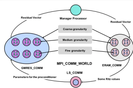
Fig. 1 gives the workflow of UCGLE and Algorithm 6 shows its implementation of three components with asynchronous communications. ERAM and GMRES components are implemented in parallel, LS Component is in serial. ERAM Component computes a de-sired number of eigenvalues, and then sends them to LS Component; LS Component uses these received eigenvalues to generate the LS pre-treatment parameters, and sends them to GMRES Component; GMRES Component uses these parameters to generate a new vec-tor as a new restarted vecvec-tor for solving linear systems. One characteristic of UCGLE is its engine to manger different components and their asynchronous communications. This engine is implemented based on MPI. UCGLE has three levels of parallelism, which is suitable for the architecture of modern large-scale platforms. The Coarse Grain/Component level, Medium Grain/inter-component level, and fine Grain/Thread level (such as GPUs and OpenMP threads) of parallelism were shown in [30].
3.2 Relation between LS Residual and Approximate Eigenvalues
Suppose that the computed convex hull by Least Squares contains eigenvalues λ1, · · · , λm,
ERAM_COMM GMRES_COMM LS_COMM Manager Processor Residual Vector MPI_COMM_WORLD Residual Vector
Some Ritz values Parameters for the preconditioner
Coarse granularity
Medium granularity
Fine granularity
Fig. 1 Workflow, asynchronous communication and different levels parallelism of UCGLE. [30]
r= k
∑
i=1 ρi(Rd(λi))lui+ n∑
i=m+1 ρi(Rd(λi))lui, (23)this residual can be divided into two parts. The first part is formulated with the first known m eigenvalues which are used to computed the convex hull by LS Component, the second part represents the residual with unknown eigenpairs.
0 360 720 1080 1440 1800 2160 2520 2880 3240
GMRES iteration step number
1e-8 1e-4 1 1e4 1e8 1e12 1e16 1e20
R
es
id
u
a
l
classic GMRES UCGLE (l = 5) UCGLE (l = 10) UCGLE (l = 18) UCGLE (l = 18,L = 2)Fig. 2 Convergence comparison of UCGLE method vs classic GMRES.
In practice, for each time preconditioning by LS polynomial method, it is often repeated for several times to improve its acceleration of convergence, that is the meaning of parameter
Algorithm 6 Implementation of Components [30]
1: function LOADERAM(input: A, ma, ν, r, εa)
2: while exit==False do
3: ERAM(A, r, ma, ν, εa, out put: Λr)
4: Send (Λr) to LS
5: if save f lg == T RU E then 6: write (Λr) to file eigenvalues.bin
7: end if
8: if Recv (X T MP) then 9: update X T MP 10: end if
11: if Recv (exit == T RU E) then 12: Send (exit) to LS Component 13: stop 14: end if 15: end while 16: end function 17: function LOADLS(input: A, b, d) 18: if Recv(Λr) then
19: LS(input: A, b, d,Λr, out put: Ad, Bd, ∆d, Hd)
20: Send (Ad, Bd, ∆d, Hd) to GMRES Component
21: end if
22: if Recv (exit == T RU E) then 23: stop
24: end if 25: end function
26: function LOADGMRES(input: A, mg, x0, b, εg, L, l, out put: xm)
27: count= 0
28: BASICGMRES(input: A, m, x0, b, out put: xm)
29: X T MP= xm
30: Send (X T MP) to ERAM Component 31: if ||b − Axm|| < εgthen
32: return xm
33: Send (exit == T RU E) to ERAM Component 34: Stop 35: else 36: if count | L then 37: if recv (Ad, Bd, ∆d, Hd) then 38: LSUpdateResidual(input : A, b, Bd, ∆d, Hd) 39: count+ + 40: end if 41: else
42: set x0= xm, and GOTO 1
43: count+ + 44: end if 45: end if
46: if Recv (exit == T RU E) then 47: stop
48: end if 49: end function
lin Equation (23). The LS polynomial preconditioning applies rd as a deflation vector for
each time GMRES restart process. Fig. 2 gives the comparison between classic GMRES and UCGLE with different values for the parameter l. As shown in this figure, the first part in Equation (23) is small since the LS method finds Rdminimizing |Rd(λ )| in the convex hull,
but not with the second part, where the residual will be rich in the eigenvectors associated with the eigenvalues outside Hk. As the number of approximated eigenvalues k increasing,
the first part will be much closer to zero, but the second part keeps still large. This results in an enormous increase of restarted GMRES preconditioned vector norm. Meanwhile, when GMRES restarts with the combination of a number of eigenvectors, the convergence will be faster even if the residual is enormous, and the convergence of GMRES can still be signif-icantly accelerated. The peaks shown in Fig. 2 for each time restart of UCGLE represent these enormous residuals. The l times repeat of rdbefore applying to next time restart can
still enlarge its norm, and the selection of l is important for the acceleration. In the example of Fig. 2, we conclude that if l is too large, the norm trends enormous, which slows down the speedup, if l is small, the acceleration may not be evident. In some situation, the precon-ditioned residual may be too large, it results that GMRES cannot converge enough before next restart. Hence the LS preconditioning can be applied each L times of GMRES restart, and the best l should be found.
3.3 Solving Linear Systems in Sequence by Recycling of Eigenvalues
After the analysis of relation between LS polynomial residual and the approximated eigen-values, it is apparent that these dominant eigenvalues used by LS Component to accelerate the convergence, can be recycled and improved from the procedure of solving system with one RHS to another, which will introduce a potential continuous improvement for solving a long sequence of linear systems.
In order to solve the sequence of linear systems Ax = btwith t ∈ 1, 2, 3, · · · . We enlarge
the Krylov subspace size mainside ERAM Component to approximate more eigenvalues.
Suppose that (ma)1for the first system, the exact implementation of ERAM Component for
t∈ 2, 3, · · · is shown in Equation (24), (ma)t is equal to the sum of (ma)t−1 and a given
constant a. And kt, the number of eigenvalues computed by ERAM Component for Ax = bt
can be described by a function f which maps the relation between (ma)tand kt. Obviously,
kt≥ kt−1. The residual (rd)tfor each restart of Ax = btwith t ∈ 2, 3, · · · is also given in (24).
(ma)t= (ma)t−1+ a kt= f (mt) (rd)t= kt
∑
i=1 (Rd(λi))lρiui+ n∑
i=kt+1 (Rd(λi))lρiuis (24)With the enlargement of ERAM Component Krylov subspace size, the more eigenvalues are calculated, then the first part of (rd)tin Equation (24) are more important, and the more
significant the acceleration will be. The continuous amelioration of convergence for solving linear systems in sequence can be gotten. With the changing of ERAM component Krylov subspace size, it may not be guaranteed to get the demanded eigenvalues in time for each restart of GMRES component if this size is too large comparing with GMRES Component Krylov subspace size. In order to improve the robustness of UCGLE, the previously calcu-lated eigenvalues are kept in memory and updated if there come the new ones. These values in memory can be utilized in case that the failure of ERAM component when the parameters are too strict. In Equation (24), we did not define the upper limit for (ma)t, which depends
on properties of operator matrices and Pgand Pafor GMRES and ERAM components.
For t ∈ 2, 3, · · · , since the eigenvalues calculated when solving Ax = bt−1 are kept in
memory, they can be used to construct an approximative solution for the current linear
sys-tem Ax = btthrough the LS polynomial method before its solve by GMRES. Obviously, this
will introduce an acceleration on the convergence for solving the linear systems in sequence. With the number of linear systems to be solved increasing, there will be more eigenvalues approximated, the initial guess vector constructed by LS component will be more accurate, and thus the speedup for solves from one to another can be still gotten. In fact, the impact of initial guess vector on the convergence is different from the restarted residual vector inside the iterative method, we propose a new parameter lt0for the initial guess generation proce-dure which is different from the l in LS preconditioning part. The residual vector (gd)tfor
Ax= btwith t ∈ 2, 3, · · · is given in Equation (25), which is constructed by the kt−1number
of eigenvalues calculated when solving Ax = bt−1.
(gd)t= kt−1
∑
i=1 (Rd(λi))l 0 tρ iui+ n∑
i=kt−1+1 (Rd(λi))l 0 tρ iui. (25)In this section, two parameters are added in order to solve linear systems in sequence using UCGLE, they are listed as below:
* (ma)t: ERAM Krylov subspace size for solving Ax = bt
* l0: times that LS polynomial applied for the generation of initial guess vector
It is predictable that this speedup for solving successive systems will stagnate after the
optimized values of maand l0are found. It is useless to use ERAM Component to
approx-imate the eigenvalues continuously. Thus Pacomputing units allocated for ERAM
Compo-nent can be redistributed to GMRES CompoCompo-nent. It is expected to get an extra speedup on the performance with more computing resources.
The Algorithm 7 gives the procedure of UCGLE for solving a sequence of linear sys-tems Ax = bt with t ∈ 1, 2, 3, · · · . Initially, Pg and Pa are respectively set to be procg and
proca. If t = 1, UCGLE loads normally the three computing components with the ERAM
component’s Krylov subspace to be (ma)1, and the initial guess vector for GMRES
compo-nent to be zero. For the solves of the successive linear systems, before the update of three
Algorithm 7 UCGLE for sequences of linear systems
1: for (t ∈ (1, 2, 3, · · · )) do 2: if (t = 1) then
3: set Pg= procgand Pa= proca
4: LOADERAM(input : A, ma, v, r, εa)
5: LOADLS(input : A, b, d)
6: LOADGMRES(input : A, mg, x0, b1, εg, L, l, out put : xm)
7: else
8: set Pg= procgand Pa= proca
9: INIT IAL GU ESS(input : A, bt, d, lt0, out put : gd t)
10: update LOADGMRES(input : A, mg, gd t, bt, εg, L, l, out put : xm)
11: update (ma)t−1by (ma)tin LOADERAM(input : A, (ma)t, v, r, εa)
12: update LOADLS(input : A, bi, d)
13: if (optmized (ma)opand lop0 found) then
14: save the eigenvalues to eigenvalues.bin 15: set Pg= procg+ proca− 1 and Pa= 1
16: INIT IAL GU ESS(input : A, bt, d, lop0 , out put : gd t) by loading eigenvalues.bin
17: LOADGMRES(input : A, mg, gd t, bt, εg, L, l, out put : xm)
18: replace LOADERAM by a simple useless function 19: LOADLS(input : A, bi, d) by loading eigenvalues.bin
20: end if 21: end if 22: end for
components, a INIT IAL GU ESS function is performed which is exactly the same as the LS component but with different parameter l0. The INIT IAL GU ESS function will generate an initial guess vector gd t. Inside GMRES component, the initial guess vector is updated by gd t
before the start of solves. And the Krylov subspace Size of ERAM Component is replaced by (ma)t. When the optimized values of (ma)opand lop0 are found, the eigenvalues are kept
into a local file eigenvalue.bin. The Pgand Paare respectively updated as procg+ proca− 1
and 1. The INIT IAL GU ESS function executes by loading eigenvalue.bin. LOADGMRES is restarted with the redeployment of its data onto procg+ proca− 1 computing units. LS
executes also with eigenvalue.bin. The retainment of 1 computing unit for ERAM Compo-nent aims to ensure the distributed and parallel implementation of UCGLE with high fault tolerance. But the inside kernel of ERAM Component is replaced by a simple function with keeping the data sending and receiving functionalities.
4 Experiments of UCGLE for Sequences of Linear Systems
In this section, we evaluate the UCGLE for solving the sequences of linear systems on the supercomputer using different generated test matrices. UCGLE with or without initial guess vector generation is compared with conventional restarted GMRES with or without avail-able preconditioners (Jacobi and SOR) in our implementations. The parallel performance on different homogeneous and heterogeneous platforms is presented in [30]. Thus this pa-per concentrates on the numerical pa-performance of UCGLE for solving non-Hermitian linear systems in sequence, and the parallel performance comparison will not be discussed. Indeed, the performance of UCGLE can achieve further improvement with unique implementation targeting at different computer architectures, but this is not the purpose of this paper. Unite
and Conquer approach(including UCGLE) is a particular programming model which
in-troduces a better performance on top of classic solvers and makes them be more suitable for modern computers. It is fair to prove the benefits of Unite and Conquer approach by comparing it with the implementations of classic solvers based on the same basic operations (distribution of matrix across the cores, parallel sparse matrix-vector operation, the orthog-onalization in Arnoldi reduction, etc.) without specific optimization for different platforms. In fact, if we optimize the parallel implementation of classic solvers and also the compo-nents (especially GMRES Component) in UCGLE at the same time, the benefits of UCGLE by reducing the global communications and promoting the asynchronization are still there.
4.1 Experimental Hardwares
UCGLE is implemented on the supercomputer Tianhe-2, installed at the National Super Computer Center in Guangzhou of China. It is a heterogeneous system made of Intel Xeon CPUs and Matrix2000, with 16000 compute nodes in total. Each node composes 2 Intel Ivy Bridge 12 cores @ 2.2 GHz. In this paper, we did not test UCGLE with co-processor Ma-trix2000 on Tianhe-2 since our implementation does not support it with good performance.
4.2 Large-scale Test Matrices Generation with Given Spectra
In order to test UCGLE with matrices of high dimensions, we use our Scalable Matrix Gen-erator with Given Spectra (SMG2S) [29, 31] to generate different test matrices. SMG2S is
an open source package implemented and optimized using MPI and C++, which allows gen-erating efficiently large-scale test matrices with customized eigenvalues by users to evaluate the impacts of spectra on the covergence of linear solvers on the large-scale platforms. Fig. 3 gives an example of SMG2S to generate test matrix. SMG2S has good scalability and ac-ceptable accuracy to keep the given spectra. One more important benefit, since the matrices are generated by SMG2S in parallel, the data are already allocated on different processes. These distributed data can be used directly for the users to efficiently evaluate the numerical methods without concerning the I/O operation.
Fig. 3 Spasity Pattern of Matrix Generated by SMG2S. [31]
4.3 Experimental Results
We evaluate UCGLE for solving sequences of linear systems using three test matrices of
size 1.572 × 10⁷generated by SMG2S with different given spectra. They are respectively
denoted as Mat1, Mat2 and Mat3. The different right-hand sides of these sequent linear systems are generated at random. The parameter l for all tests using UCGLE keeps the same as 10. The numbers of process for GMRES and ERAM Components in UCGLE are respectively 768 and 384. Five methods are compared in the experiments, and the notations of different methods are given as below:
– GMRES: classic restarted GMRES;
– GMRES+SOR or SOR: GMRES with SOR preconditioner; – GMRES+Jacobi or Jacobi: GMRES with Jacobi preconditioner;
– UCGLE without initial guess: UCGLE without using previously obtained eigenvalues to generate an initial guess vector for the next system by LS polynomial method; – UCGLE with initial guess: UCGLE using previously obtained eigenvalues to generate
an initial guess vector for the next systems by LS polynomial method.
ERAM and LS components in UCGLE demand additional computing units. It is un-fair to test only the conventional methods of their numbers of CPUs equal to the number of GMRES components in UCGLE. Therefore, experiments have also been tested that the numbers of computing units of the classical iterative method are equal to the total CPU in
1 2 3 4 5 6 7 8 9
Right-hand sides index
0.0 0.5 1.0 1.5 2.0 2.5 3.0 3.5 E xe cu ti o n T im e( s) (a)
UCGLE without initial guess GMRES
SOR
Jacobi
UCGLE with initial guess, ERAM Subspace (10-30) GMRES with total CPUs
SOR with total CPUs Jacobi with total CPUs
5 6 7 8 9
Right-hand sides index
0.0 0.5 1.0 1.5 2.0 2.5 3.0 3.5 E xe cu ti o n T im e( s) (b)
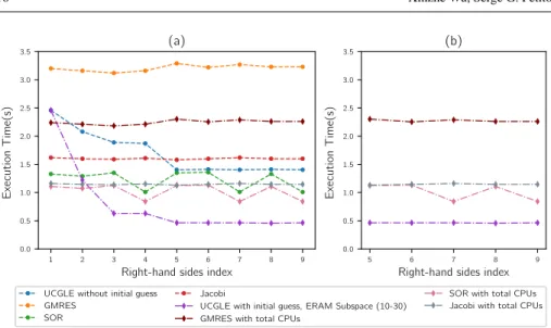
Fig. 4 Mat1: time comparison for solving a sequence of linear systems. (a) shows the solution time for 9 sequent linear systems; (b) shows the cases extracted from (a) after the good selection of parameters in UCGLE.
UCGLE (hence, the CPUs for GMRES and ERAM components are included). In the cap-tions of figures, a given method ”with total CPUs” means that its number of CPUs equals to the total CPU in UCGLE. The time comparisons for solving nine sequent linear systems of Mat1, Mat2 and Mat3 are given respectively in Fig. 4 (a), Fig. 5 (a) and Fig. 6 (a), the comparison of the number of iteration for convergence are respectively given in Table 1, Table 2 and Table 3. From these three tables, we conclude that UCGLE has the ability to speed up the convergence to solve linear systems with test matrices comparing with the con-ventional methods. The generation of initial vectors using the eigenvalues for subsequent linear systems can still speed up the convergence over the UCGLE without initial guess.
Table 1 Mat1: iterative step comparison for solving a sequence of linear systems.
Method 1 2 3 4 5 6 7 8 9 GMRES 509 505 501 505 527 510 523 516 518 GMRES+SOR 169 165 172 130 172 173 130 170 130 GMRES+Jacobi 274 273 270 276 269 274 280 276 273 UCGLE w/o initial guess 120 90 90 90 90 90 90 90 90 UCGLE with initial guess 120 36 35 35 36 36 36 33 35
For the tests of Mat1, the GMRES restart size is 30, the Krylov subspace of ERAM Component for solving the first three linear systems are respectively 10, 20 and 30, the size of this subspace of ERAM for the remaining systems keeps being 30. For the tests of Mat2, the GMRES restart size is 300, the Krylov subspace of ERAM Component for solving the first three linear systems are respectively 100, 150 and 200, the size of this subspace of ERAM for the remaining systems keeps being 200. For the cases that UCGLE
with initial guess, the parameter l0for Mat1 and Mat2 keeps 30. With the augmentation of the size of ERAM Krylov subspace, there will be more eigenvalues to be approximated, and we find that there is acceleration with the accumulation of more eigenvalues for both the case UCGLE with and without initial guess. The influence of subspace of ERAM can be found through the curves of UCGLE with/without initial guess in Fig. 4 (a) and Fig. 5 (a). However, it is not practical to enlarge too much the Krylov subspace of ERAM to approximated more eigenvalues, since if it is too large, it takes too much time by ERAM, LS Component cannot receive the eigenvalues in time, thus it will be difficult for the GMRES Component to perform the LS preconditioning for it each time restart.
1 2 3 4 5 6 7 8 9
Right-hand sides index
10 20 30 40 50 60 E xe cu ti o n T im e( s) (a)
UCGLE without initial guess GMRES
SOR
Jacobi
UCGLE with initial guess, ERAM Subspace (150-300) GMRES with total CPUs
SOR with total CPUs Jacobi with total CPUs
5 6 7 8 9
Right-hand sides index
10 20 30 40 50 60 E xe cu ti o n T im e( s) (b)
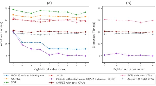
Fig. 5 Mat2: time comparison for solving a sequence of linear systems. (a) shows the solution time for 9 sequent linear systems; (b) shows the cases extracted from (a) after the good selection of parameters in UCGLE.
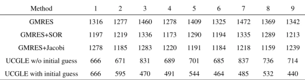
Table 2 Mat2: iterative step comparison for solving a sequence of linear systems.
Method 1 2 3 4 5 6 7 8 9 GMRES 1316 1277 1460 1278 1409 1325 1472 1369 1342 GMRES+SOR 1197 1219 1336 1173 1290 1194 1335 1289 1213 GMRES+Jacobi 1278 1185 1283 1220 1191 1184 1218 1159 1239 UCGLE w/o initial guess 666 671 831 689 701 685 837 736 714 UCGLE with initial guess 666 595 470 491 544 464 485 532 440
For the tests of Mat3, the GMRES restart size is 150, and the Krylov subspace size of ERAM Components keeps the same to be 200. Meanwhile, for the 2nd, 3rd and 4th linear systems, the parameter l0of initial guess are respectively 20, 30 and 40, for the remaining linear systems, this parameter keeps 40. For the solving the linear systems by UCGLE with
initial guess, we can find that with the augmentation of l0, the iteration numbers for the first four linear systems decrease quickly from 360 to 283 with approximately 1.3× speedup. For Mat3, SOR preconditioned GMRES is already good, but UCGLE with initial guess has still about 2.2× speedup of convergence. Even in the case that the computing unit number of SOR preconditioned GMRES equals to the total number of UCGLE, UCGLE with initial
guess can achieve 2.2× of execution time speedup. The augmentation of the parameter l0
has a strong impact on the convergence. Since the Mat3 is generated with the clustered eigenvalues which are randomly distributed inside a fixed region of the real-imaginary plan, if l0is larger, it can be seen as there are much more eigenvalues generated, even they are not very accurate compared with the real ones. The inaccuracy of eigenvalues can result in the enlargement of the norm in Equation (24), but it can still very quickly converge. It is effective to generate an initial guess vector with very large l0, but not the same case for the parameter l inside each preconditioning, since the too many times of repeats for each time restart will amplify quicky this inaccuracy of norm, and it is easy to result in the difficulties of convergence.
In order to use UCGLE for solving a large number of linear systems in sequence, it is necessary to choose the suitable parameters by the evaluation of a small number of sequent linear systems. After the selection of parameters, we compare the best cases of each method with the least time consumption. The results for three test matrices are shown in Fig. 4 (b), Fig. 5 (b) and Fig. 6 (b). We conclude that for Mat1, UCGLE with initial guess has about 4.4× for the acceleration of convergence and 1.7× for the speedup of execution time. For Mat2, it has about 4.3× acceleration for the convergence and 2.6× for the speedup of time. For Mat3, it has about 3.2× acceleration for the convergence and 2.0× for the speedup of execution time.
1 2 3 4 5 6 7 8 9
Right-hand sides index
5 10 15 20 25 E xe cu ti o n T im e( s) (a)
UCGLE without initial guess GMRES
SOR
Jacobi
UCGLE with initial guess, ERAM Subspace (10-30) GMRES with total CPUs
SOR with total CPUs Jacobi with total CPUs
5 6 7 8 9
Right-hand sides index
5 10 15 20 25 E xe cu ti o n T im e( s) (b)
Fig. 6 Mat3: time comparison for solving a sequence of linear systems. (a) shows the solution time for 9 sequent linear systems; (b) shows the cases extracted from (a) after the good selection of parameters in UCGLE.
In conclusion, the UCGLE, especially it with the recycling eigenvalues to generate initial guess vector using the eigenvalues, can significantly accelerate the convergence and reduce
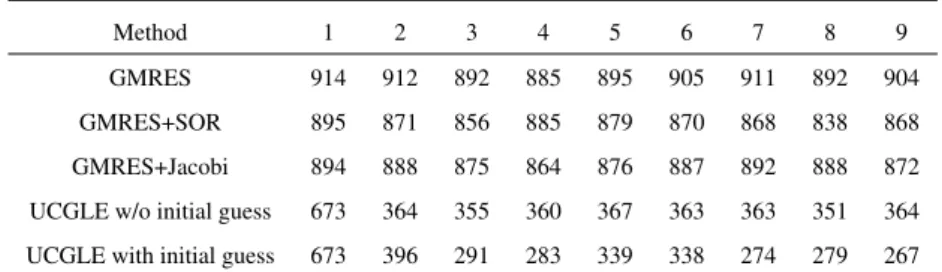
Table 3 Mat3: iterative step comparison for solving a sequence of linear systems.
Method 1 2 3 4 5 6 7 8 9 GMRES 914 912 892 885 895 905 911 892 904 GMRES+SOR 895 871 856 885 879 870 868 838 868 GMRES+Jacobi 894 888 875 864 876 887 892 888 872 UCGLE w/o initial guess 673 364 355 360 367 363 363 351 364 UCGLE with initial guess 673 396 291 283 339 338 274 279 267
the time consumption for solving a sequence of linear systems. However, the time employed by the LS iterative recurrence, especially a small number of Sparse Matrix-Vector Product operations inside makes the time speedup not consistent with the convergence speedup. For example, in Table 3, UCGLE with initial guess has almost 3.0× acceleration on the convergence over the classic GMRES for solving the 3rd linear system. But it has only about 2.0× acceleration on the performance in the case that the classic GMRES and GMRES Component inside UCGLE have the same number of computing units. It is caused by the recurrence of LS iterations to perform the preconditioning on GMRES Component after receiving the parameters from LS Component. Nevertheless, UCGLE is more efficient to solve the sequences of linear systems, and with its distributed and parallel communication framework, it is a good candidate for solving non-Hermitian linear systems in sequence on much larger machines.
5 Conclusion and Perspective
This paper proposes an extended version of the distributed parallel method UCGLE, which is used to solve a large number of linear systems with unique matrices and different right sides on a large platform. UCGLE method was proposed to solve large-scale linear sys-tems on modern computing platforms, which is able to minimize the global communication, cover the synchronous points in the parallel implementation, improve the fault tolerance and reusability and speed up the convergence. In this paper, It is proved this developed variant of UCGLE method can solve the linear systems with special spectral distribution in se-quence more effectively than several preconditioned iterative methods. The recycling of a small group of dominant eigenvalues and generating initial guess vector using them by Least Squares polynomial method has a significant impact on the performance improvement for solving continuous linear systems.
Various parameters have an impact on the convergence. Thus, the auto-tuning scheme is required in the future work, where the systems can select different Krylov subspace di-mensions, numbers of eigenvalues to be computed, degrees of Least Squares polynomial according to different linear systems and cluster architectures.
References
1. Abdel-Rehim AM, Morgan RB, Wilcox W (2014) Improved seed methods for symmet-ric positive definite linear equations with multiple right-hand sides. Numesymmet-rical Linear Algebra with Applications 21(3):453–471
2. Arnoldi WE (1951) The principle of minimized iterations in the solution of the matrix eigenvalue problem. Quarterly of applied mathematics 9(1):17–29
3. Baker AH, Dennis JM, Jessup ER (2006) On improving linear solver performance: A block variant of gmres. SIAM Journal on Scientific Computing 27(5):1608–1626 4. Bellavia S, Morini B (2001) A globally convergent newton-gmres subspace method for
systems of nonlinear equations. SIAM Journal on Scientific Computing 23(3):940–960 5. Benner P, Feng L (2011) Recycling krylov subspaces for solving linear systems with successively changing right-hand sides arising in model reduction. In: Model Reduction for Circuit Simulation, Springer, pp 125–140
6. Brown PN, Saad Y (1990) Hybrid krylov methods for nonlinear systems of equations. SIAM Journal on Scientific and Statistical Computing 11(3):450–481
7. Calvetti D, Reichel L (1994) Application of a block modified chebyshev algorithm to the iterative solution of symmetric linear systems with multiple right hand side vectors. Numerische Mathematik 68(1):3–16
8. Craig RR, Hale AL (1988) Block-krylov component synthesis method for structural model reduction. Journal of Guidance, Control, and Dynamics 11(6):562–570
9. Dongarra J, Hittinger J, Bell J, Chacon L, Falgout R, Heroux M, Hovland P, Ng E, Webster C, Wild S (2014) Applied mathematics research for exascale computing. Tech. rep., Lawrence Livermore National Laboratory (LLNL), Livermore, CA
10. Emad N, Petiton S (2016) Unite and conquer approach for high scale numerical com-puting. Journal of Computational Science 14:5–14
11. Essai A, Berg´ere G, Petiton SG (1999) Heterogeneous parallel hybrid gmres/ls-arnoldi method. In: PPSC
12. Flueck AJ, Chiang HD (1998) Solving the nonlinear power flow equations with an inexact newton method using gmres. IEEE Transactions on Power Systems 13(2):267– 273
13. Gu GD (2002) A seed method for solving nonsymmetric linear systems with multiple right-hand sides. International journal of computer mathematics 79(3):307–326 14. Gullerud AS, Dodds Jr RH (2001) Mpi-based implementation of a pcg solver using an
ebe architecture and preconditioner for implicit, 3-d finite element analysis. Computers & Structures 79(5):553–575
15. Gutknecht MH (2006) Block krylov space methods for linear systems with multiple right-hand sides: an introduction
16. He H, Berg`ere G, Petiton S (2006) A hybrid gmres/ls-arnoldi method to accelerate the parallel solution of linear systems. Computers & Mathematics with Applications 51(11):1647–1662
17. Jolivet P, Tournier PH (2016) Block iterative methods and recycling for improved scala-bility of linear solvers. In: SC16-International Conference for High Performance Com-puting, Networking, Storage and Analysis
18. Kershaw DS (1978) The incomplete choleskyconjugate gradient method for the iterative solution of systems of linear equations. Journal of Computational Physics 26(1):43–65 19. Kilmer ME, De Sturler E (2006) Recycling subspace information for diffuse optical
tomography. SIAM Journal on Scientific Computing 27(6):2140–2166
20. Knoll DA, Keyes DE (2004) Jacobian-free newton–krylov methods: a survey of ap-proaches and applications. Journal of Computational Physics 193(2):357–397
21. Papadrakakis M, Smerou S (1990) A new implementation of the lanczos method in lin-ear problems. International Journal for Numerical Methods in Engineering 29(1):141– 159
22. Parks ML, De Sturler E, Mackey G, Johnson DD, Maiti S (2006) Recycling krylov subspaces for sequences of linear systems. SIAM Journal on Scientific Computing 28(5):1651–1674
23. Saad Y (1987) Least squares polynomials in the complex plane and their use for solving nonsymmetric linear systems. SIAM Journal on Numerical Analysis 24(1):155–169 24. Saad Y (1987) On the lanczos method for solving symmetric linear systems with several
right-hand sides. Mathematics of computation 48(178):651–662
25. Saad Y (2011) Numerical Methods for Large Eigenvalue Problems: Revised Edition. SIAM
26. Saad Y, Schultz MH (1986) Gmres: A generalized minimal residual algorithm for solv-ing nonsymmetric linear systems. SIAM Journal on scientific and statistical computsolv-ing 7(3):856–869
27. Simoncini V, Gallopoulos E (1995) An iterative method for nonsymmetric systems with multiple right-hand sides. SIAM Journal on Scientific Computing 16(4):917–933 28. Smith CF, Peterson AF, Mittra R (1989) A conjugate gradient algorithm for the
treat-ment of multiple incident electromagnetic fields. IEEE Transactions on Antennas and Propagation 37(11):1490–1493
29. WU X (2018) SMG2S Manual v1.0. Technical report, Maison de la Simulation 30. Wu X, Petiton SG (2018) A distributed and parallel asynchronous unite and conquer
method to solve large scale non-hermitian linear systems. In: Proceedings of the Inter-national Conference on High Performance Computing in Asia-Pacific Region, ACM, New York, NY, USA, HPC Asia 2018, pp 36–46, DOI 10.1145/3149457.3154481 31. WU X, Petiton S, Lu Y (2018) A Parallel Generator of Non-Hermitian Matrices
com-puted from Given Spectra. In: VECPAR 2018: 13th International Meeting on High Per-formance Computing for Computational Science, So Paulo, Brazil
32. Ye Z, Zhu Z, Phillips JR (2008) Generalized krylov recycling methods for solution of multiple related linear equation systems in electromagnetic analysis. In: Proceedings of the 45th annual Design Automation Conference, ACM, pp 682–687
33. Zhang Y, Bergere G, Petiton S (2008) Large scale parallel hybrid gmres method for the linear system on grid system. In: Parallel and Distributed Computing, 2008. ISPDC’08. International Symposium on, IEEE, pp 244–249
![Fig. 3 Spasity Pattern of Matrix Generated by SMG2S. [31]](https://thumb-eu.123doks.com/thumbv2/123doknet/13307985.398529/16.892.134.601.305.523/fig-spasity-pattern-matrix-generated-smg-s.webp)