Model constraints on the anthropogenic carbon budget of the Arctic Ocean

HAL Id: hal-02165633

https://hal.sorbonne-universite.fr/hal-02165633

Submitted on 26 Jun 2019

HAL is a multi-disciplinary open access

archive for the deposit and dissemination of

sci-entific research documents, whether they are

pub-lished or not. The documents may come from

teaching and research institutions in France or

abroad, or from public or private research centers.

L’archive ouverte pluridisciplinaire HAL, est

destinée au dépôt et à la diffusion de documents

scientifiques de niveau recherche, publiés ou non,

émanant des établissements d’enseignement et de

recherche français ou étrangers, des laboratoires

publics ou privés.

of the Arctic Ocean

Jens Terhaar, James Orr, Marion Gehlen, Christian Éthé, Laurent Bopp

To cite this version:

Jens Terhaar, James Orr, Marion Gehlen, Christian Éthé, Laurent Bopp. Model constraints on the

anthropogenic carbon budget of the Arctic Ocean. Biogeosciences, European Geosciences Union, 2019,

16 (11), pp.2343-2367. �10.5194/bg-16-2343-2019�. �hal-02165633�

https://doi.org/10.5194/bg-16-2343-2019 © Author(s) 2019. This work is distributed under the Creative Commons Attribution 4.0 License.

Model constraints on the anthropogenic carbon budget

of the Arctic Ocean

Jens Terhaar1, James C. Orr1, Marion Gehlen1, Christian Ethé2, and Laurent Bopp3

1_{Laboratoire des Sciences du Climat et de l’Environnement, LSCE/IPSL, CEA-CNRS-UVSQ,}

Université Paris-Saclay, Gif-sur-Yvette, France

2_{Institut Pierre et Simon Laplace, Paris, France}

3_{LMD/IPSL, Ecole Normale Supérieure/PSL Research University, CNRS, Ecole Polytechnique,}

Sorbonne Université, Paris, France

Correspondence: Jens Terhaar (jens.terhaar@lsce.ipsl.fr) Received: 11 June 2018 – Discussion started: 25 June 2018

Revised: 12 March 2019 – Accepted: 16 April 2019 – Published: 7 June 2019

Abstract. The Arctic Ocean is projected to experience not only amplified climate change but also amplified ocean acid-ification. Modeling future acidification depends on our abil-ity to simulate baseline conditions and changes over the in-dustrial era. Such centennial-scale changes require a global model to account for exchange between the Arctic and sur-rounding regions. Yet the coarse resolution of typical global models may poorly resolve that exchange as well as criti-cal features of Arctic Ocean circulation. Here we assess how simulations of Arctic Ocean storage of anthropogenic car-bon (Cant), the main driver of open-ocean acidification,

dif-fer when moving from coarse to eddy-admitting resolution in a global ocean-circulation–biogeochemistry model (Nu-cleus for European Modeling of the Ocean, NEMO; Pelagic Interactions Scheme for Carbon and Ecosystem Studies, PISCES). The Arctic’s regional storage of Cant is enhanced

as model resolution increases. While the coarse-resolution model configuration ORCA2 (2◦) stores 2.0 Pg C in the Arc-tic Ocean between 1765 and 2005, the eddy-admitting ver-sions ORCA05 and ORCA025 (1/2◦ and 1/4◦) store 2.4 and 2.6 Pg C. The difference in inventory between model resolutions that is accounted for is only from their diver-gence after 1958, when ORCA2 and ORCA025 were ini-tialized with output from the intermediate-resolution config-uration (ORCA05). The difference would have been larger had all model resolutions been initialized in 1765 as was ORCA05. The ORCA025 Arctic Cant storage estimate of

2.6 Pg C should be considered a lower limit because that model generally underestimates observed CFC-12

concen-trations. It reinforces the lower limit from a previous data-based approach (2.5 to 3.3 Pg C). Independent of model res-olution, there was roughly 3 times as much Cant that

en-tered the Arctic Ocean through lateral transport than via the flux of CO2across the air–sea interface. Wider comparison

to nine earth system models that participated in the Cou-pled Model Intercomparison Project Phase 5 (CMIP5) re-veals much larger diversity of stored Cantand lateral

trans-port. Only the CMIP5 models with higher lateral transport obtain Cantinventories that are close to the data-based

esti-mates. Increasing resolution also enhances acidification, e.g., with greater shoaling of the Arctic’s average depth of the aragonite saturation horizon during 1960–2012, from 50 m in ORCA2 to 210 m in ORCA025. Even higher model res-olution would likely further improve such estimates, but its prohibitive costs also call for other more practical avenues for improvement, e.g., through model nesting, addition of coastal processes, and refinement of subgrid-scale parame-terizations.

1 Introduction

The Arctic is experiencing amplified ocean acidification (Steinacher et al., 2009) and amplified climate change (Bekryaev et al., 2010), both of which may affect the marine ecosystem (Gattuso and Hansson, 2011). The main driver of the ongoing acidification of the open ocean is the increase in atmospheric CO2 during the industrial era and the ensuing

uptake of anthropogenic carbon from the atmosphere. Al-though this absorbed anthropogenic carbon cannot be mea-sured directly, being dominated by the natural component, it has been estimated from other oceanographic data.

For instance, Gruber et al. (1996) developed the 1C∗ method, building on seminal studies (Brewer, 1978; Chen and Millero, 1979) and their criticism (Broecker et al., 1985) as well as large new global data sets with improved CO2

sys-tem measurements. That back-calculation method first calcu-lates the total dissolved inorganic carbon (CT) at equilibrium

with the atmosphere before the water parcel is subducted. The preformed CTis then corrected for changes due to

bio-logical activity, as estimated from measurements of dissolved oxygen, total alkalinity (AT), and nutrients, after which an

estimate of preindustrial carbon is removed, finally yielding 1C∗. Yet the 1C∗method’s assumption of a constant air–sea CO2disequilibrium appears problematic in the high latitudes

(Orr et al., 2001).

A second approach approximates the invasion of anthro-pogenic CO2into the interior ocean by a transient time

dis-tribution (TTD) method, itself constrained by observations of transient tracers such as CFC-12 or SF6(Hall et al., 2002;

Waugh et al., 2004). A third approach uses a Green’s func-tion instead of a TTD while also exploiting multiple transient tracers to assess the ocean’s temporally changing distribution of anthropogenic carbon (Khatiwala et al., 2009). A compari-son of these methods suggests that by 2010 the ocean had ab-sorbed 155 ± 31 Pg C of anthropogenic carbon, around one-third of all emitted anthropogenic carbon (Khatiwala et al., 2013)

Less attention has been paid to anthropogenic carbon stor-age in the Arctic. Sabine et al. (2004) estimated that the Arctic Ocean had absorbed 4.9 Pg C by 1994. Yet with-out estimates for anthropogenic carbon in the Arctic itself, Sabine et al. (2004) scaled the Arctic inventory to be 5 % of their 1C∗-based estimate for global anthropogenic carbon storage, assuming the same Arctic : global ocean ratio as in the global gridded distribution of observed CFC-12 (Willey et al., 2004). More recently, Tanhua et al. (2009) used Arc-tic observations of CFC-11, CFC-12, and SF6and the TTD

approach, revising the former Arctic anthropogenic carbon storage estimate downward to a range of 2.5 to 3.3 Pg C for year 2005. With that estimate, they emphasized that while the Arctic Ocean represents only 1 % of the global ocean volume, it stores 2 % of the global ocean’s anthropogenic carbon. Although these numbers are relatively small, Arctic concentrations of anthropogenic CTmust be relatively large,

thus driving enhanced acidification in the Arctic Ocean. No other approaches have been used in the Arctic.

To provide an alternate approach to estimate anthro-pogenic carbon in the Arctic and to assess its budget and the mechanisms that control it, one could make carbon cy-cle simulations over the industrial era with a coupled ocean-circulation–biogeochemical model. A global-scale model configuration would be needed to account for the Arctic in

Figure 1. CFC-12 stations along the AOS94 (red) and Beringia 2005 expeditions (white). Other colors indicate the bathymetry of the Arctic Ocean, while the four dashed black lines show the bound-aries of the Arctic Ocean domain used in this study.

the context of the global carbon cycle, while avoiding ar-tifacts from lateral boundary conditions that must be im-posed in regional models. Yet typical ocean general circu-lation models have coarse resolution, which may be insuffi-cient to adequately represent Arctic Ocean bathymetry, shelf, slopes, and ridges, all of which affect Arctic Ocean circula-tion (Rudels et al., 1994).

The bathymetry of the Arctic Ocean differs from that in other oceans in part because of the preponderance of shelf seas, comprising 53 % of the total surface area (Jakobsson, 2002) (Fig. 1). The remaining 47 % of its surface area cov-ers 95 % of the total volume of the Arctic Ocean, split across four deep basins: the Nansen Basin, the Amundsen Basin, the Makarov Basin, and the Canadian Basin. Water masses enter these deep basins via (1) deep inflow from the At-lantic through the Fram Strait into the Nansen Basin, (2) in-flow from the Barents Sea that sinks into the Nansen Basin through the St. Anna Trough, as cooling increases density, and (3) transport from density flows along the continental shelves that are driven by brine rejection from sea-ice forma-tion (Jones et al., 1995). These three local transfers are dif-ficult to resolve in coarse-resolution models, e.g., local den-sity flows necessitate much higher resolution (Proshutinsky et al., 2016). Model resolution also affects the simulated in-terior circulation of the Arctic Ocean by its connection to the global ocean circulation via four relatively narrow and shal-low passages: (1) the Canadian Archipelago, (2) the Fram Strait, (3) the Barents Sea Opening, and (4) the Bering Strait (Aksenov et al., 2016). Lateral exchange of water, carbon, and nutrients across these sections also affects Arctic Ocean

primary production and acidification (Popova et al., 2013; Luo et al., 2016).

Here our aim is to use a three-dimensional model to help refine the estimate of the total anthropogenic carbon in the Arctic Ocean while assessing the dominant pathways by which anthropogenic carbon enters the Arctic Ocean and the importance of that lateral input relative to the air–sea flux. Three simulations made at increasingly higher lateral grid resolution are aimed at assessing the extent to which the coarse resolution used by typical global ocean models may need to be improved to adequately estimate storage of an-thropogenic carbon in the Arctic Ocean and associated ocean acidification.

2 Methods

Multiple global simulations were made to assess Cantin the

ocean. Simulations were made with a state-of-the-art ocean-circulation–biogeochemical model at three resolutions over the industrial period since the mid-19th century, i.e., as is typ-ical of recent model comparison efforts. Longer simulations were also made at the same resolutions with a less costly (and less precise) perturbation approach to correct for the missing anthropogenic carbon given that the actual industrial era be-gan about a century earlier (mid-18th century). The highest-resolution configuration used an unprecedented lateral grid spacing for such long, global, biogeochemical simulations, although its cost meant its effect could be assessed only over 1958–2012.

2.1 Models

For our study, we used the global ocean circulation model NEMO-v3.2 (Nucleus for European Modeling of the Ocean – version 3.2). The NEMO model has three parts: (1) the ocean dynamics and thermodynamics model Océan Paral-lélisé (OPA) (Madec, 2008), (2) the Louvain-la-Neuve Sea Ice Model (LIM) (Vancoppenolle et al., 2009), and (3) the passive tracer module TOP. This physical model is cou-pled via TOP to version 1 of PISCES (Pelagic Interac-tions Scheme for Carbon and Ecosystem Studies) (Aumont and Bopp, 2006). For this study we used NEMO at three resolutions: a laminar 2◦ configuration (ORCA2) typical of coarse-resolution ocean models (Madec et al., 1998), which does not resolve eddies; an intermediate 0.5◦ config-uration (ORCA05) that just begins to allow eddies to ap-pear spontaneously (Bourgeois et al., 2016); and a higher-resolution, eddy-admitting version, i.e., a 0.25◦ configura-tion (ORCA025), which is still not eddy resolving (Barnier et al., 2006). The highest-resolution simulation is referred to as ORCA025-G70 in the DRAKKAR ensemble.

All three configurations have a tripolar, curvilinear hori-zontal grid. One grid pole (singularity) is located at the geo-graphical South Pole while the conventional North Pole grid

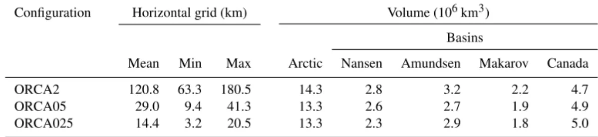
singularity over the Arctic Ocean has been replaced by two grid singularities, both displaced over land – one over Canada and the other over Russia (Madec et al., 1998) – thereby saving computational costs and avoiding numerical artifacts. From 90◦S to 20◦N, the grid is a normal Mercator grid; north of 20◦N, it is distorted into ellipses to create the two northern singularities (Barnier et al., 2006; Madec, 2008). The grid size changes depending on resolution and location (Table 1). The mean horizontal grid size in the Arctic Ocean (average length of the four horizontal edges of surface grid cells in the Arctic Ocean) is 121 km in ORCA2, 29 km in ORCA05, and 14 km in ORCA025. The smallest horizontal grid size in the Arctic is 63 km in ORCA2, 9 km in ORCA05, and 3 km in ORCA025.

Vertically, all three model configurations have the same discretization, where the full-depth water column is divided into 46 levels whose thicknesses vary from 6 m (top level) to 249 m (level 45), but the latter can reach up to 498 m, be-ing extended into level 46 as a function of the bathymetry (partial steps). For its bathymetry, the ocean model relies on the 2 min bathymetry file ETOPO2 from the National Geo-physical Data Center, which is based on satellite-derived data (Smith and Sandwell, 1997) except for the highest latitudes: the International Bathymetric Chart of the Arctic Ocean (IB-CAO) data are used in the Arctic (Jakobsson et al., 2000) and Antarctic Bedrock Mapping (BEDMAP) bathymetric data are used for the Southern Ocean south of 72◦S (Lythe and Vaughan, 2001). To interpolate the bathymetry on the model grid, the median of all data points in one model grid cell was computed. NEMO uses the partial-step approach for the model to better match the observed topography. In this ap-proach, the bathymetry of the model is not tied directly to the bottom edge of the deepest ocean grid level, which varies with latitude and longitude; rather, the deepest ocean grid level for each column of grid cells is partially filled in to better match the observed ocean bathymetry (Barnier et al., 2006).

The lateral isopycnal diffusion and viscosity coefficients were chosen depending on the resolution (Table 2). In ORCA2, a Laplacian viscosity operator was used, whereas a bi-Laplacian operator was used in ORCA05 and ORCA025. To simulate the effect of eddies on the mean advective trans-port in the two coarser-resolution configurations, the eddy parameterization scheme of Gent and Mcwilliams (1990) was applied with eddy diffusion coefficients indicated in Ta-ble 2. Vertically, the same eddy viscosity (1.2×10−4m2s−1) and diffusivity coefficients (1.2 × 10−5m2s−1) were used in all three resolutions.

The biogeochemical model PISCES (Aumont and Bopp, 2006) includes four plankton functional types: two phyto-plankton types (nanophytophyto-plankton and diatoms) and two zooplankton types (micro- and meso-zooplankton). The growth of phytoplankton is limited by the availability of five nutrients: nitrate, ammonium, total dissolved inorganic phosphorus PT, total dissolved silicon SiT, and iron. The

Table 1. Grid size in the Arctic Ocean and volumes by basin as a function of model resolution.

Configuration Horizontal grid (km) Volume (106km3) Basins

Mean Min Max Arctic Nansen Amundsen Makarov Canada ORCA2 120.8 63.3 180.5 14.3 2.8 3.2 2.2 4.7 ORCA05 29.0 9.4 41.3 13.3 2.6 2.7 1.9 4.9 ORCA025 14.4 3.2 20.5 13.3 2.3 2.9 1.8 5.0

Table 2. Coefficients for lateral diffusivity, lateral viscosity, and eddy-induced velocity for ORCA2, ORCA05, and ORCA025.

Configuration Lateral diffusivity Lateral viscositya Eddy-induced velocity ORCA2b 2000 m2s−1 4 × 104m2s−1c 2000 m2s−1

ORCA05 600 m2s−1 −4 × 1011m2s−1 1000 m2s−1 ORCA025 300 m2s−1 −1.5 × 1011m2s−1 none

a_{In ORCA2, a Laplacian viscosity operator was used, whereas a bi-Laplacian operator was used in ORCA05 and}

ORCA025.b_{Lateral diffusivity and viscosity coefficients decrease towards the poles proportional to the grid size.} c_{Reduced to 2100 m}2_s−1_{in the tropics (except along western boundaries).}

nanophytoplankton and diatoms are distinguished by their need for all nutrients, with only diatoms requiring silicon. While the Fe : C and Chl : C ratios of both phytoplankton groups as well as the Si : C ratio of diatoms are predicted prognostically by PISCES, the remaining macronutrient ra-tios are held constant at C : N : P = 122 : 16 : 1 (Takahashi et al., 1985). The same ratio holds for nonliving compart-ments: dissolved organic matter (DOM) and both small and large sinking particles, which differ in their sinking ve-locity. In PISCES, nutrients are supplied by three external pathways: atmospheric dust deposition, river delivery, and sediment mobilization of iron. Dust deposition was taken from a simulation by Tegen and Fung (1995). River dis-charge of CT and dissolved organic carbon (DOC) is based

on the Global Erosion Model (GEM) by Ludwig et al. (1998). Riverine DOC was assumed to be entirely labile, be-ing instantaneously transformed into CT as soon as it

en-ters the ocean. River delivery of the other four nutrients (Fe, N, P, and Si) was calculated from riverine CT

deliv-ery, assuming constant ratios of C : N : P : Si : Fe = 320 : 16 : 1 : 53.3 : 3.64 ×10−3 (Meybeck, 1982). For sediment mo-bilization, the dissolved iron input was parameterized as 2 µmol Fe m−2d−1for depths shallower than 386 m and de-creases exponentially with depth following Moore et al. (2004).

2.2 Biogeochemical simulations

For initial conditions, we used observational climatologies for (1) temperature and salinity (a combined product from Barnier et al., 2006), (2) dissolved oxygen and nutrients (nitrate, PT, and SiT) from the 2001 World Ocean Atlas

(Conkright et al., 2002), and (3) preindustrial CT and AT

from the observation-based Global Data Analysis Product (GLODAP) (Key et al., 2004). As comparable observational climatologies for DOC and iron are lacking, those variables were initialized from the output of a 3000-year spin-up of an ORCA2 simulation including PISCES. Other tracers have short recycling times and were thus initialized with globally uniform constants.

For physical boundary conditions, all simulations were forced with the same DRAKKAR forcing set (DFS) con-structed originally by Brodeau et al. (2010) and routinely up-dated. This historical reanalysis-based forcing data set pro-vides surface air temperature and humidity at 2 m, wind fields at 10 m, shortwave and longwave radiation, and the net surface freshwater flux (evaporation minus precipitation). It covers 55 years, including 1958–2001 from version 4.2 and 2002–2012 from version 4.4.

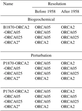
A 50-year spin-up was first made from rest in the ORCA05 NEMO-PISCES model (coupled circulation– biogeochemistry), after initializing the model variables with the abovementioned fields. The resulting simulated physi-cal and biogeochemiphysi-cal fields were then used to initialize the ORCA05 NEMO-PISCES simulations in 1870, and that model was subsequently integrated over 1870–1957. Since no atmospheric reanalysis is available during that period, we simply looped the DRAKKAR Forcing Set. Then, at the be-ginning of 1958, the ORCA05 simulated fields were inter-polated to the ORCA2 and ORCA025 grids, and simulations were continued in each of the three configurations from 1958 to 2012. We refer to these simulations as B1870-ORCA2, B1870-ORCA05, and B1870-ORCA025 (Table 3), where the first letter refers to the type of simulation (B for biogeochem-ical), the following four numbers refer to the initialization

Table 3. Set of simulations.

Name Resolution Before 1958 After 1958 Biogeochemical

B1870-ORCA2 ORCA05 ORCA2 -ORCA05 ORCA05 ORCA05 -ORCA025 ORCA05 ORCA025 -ORCA2∗ ORCA2 ORCA2

Perturbation

P1870-ORCA2 ORCA05 ORCA2 -ORCA05 ORCA05 ORCA05 -ORCA025 ORCA05 ORCA025 -ORCA2∗ ORCA2 ORCA2

P1765-ORCA2 ORCA05 ORCA2 -ORCA05 ORCA05 ORCA05 -ORCA025 ORCA05 ORCA025 -ORCA2∗ ORCA2 ORCA2

year, and the remainder refers to the resolution used over 1958–2012.

The initialization of the ORCA2 and ORCA025 models in 1958 with interpolated fields from ORCA05 introduces an error into the results from ORCA2 and B1870-ORCA025. To estimate this branching error in the low-resolution model, we also made a simulation using ORCA2 from 1870 to 2012 (referred to as B1870-ORCA2∗) and compared it to B1870-ORCA2 (initialized in 1958 with output from ORCA05). This strategy was not possible for ORCA025 because running ORCA025 with PISCES over 1870–2012 is too costly.

For each member of this “B” class of simulations, we ac-tually made two types of runs: historical and control, both forced with the same reanalysis fields. Those two runs differ only in their atmospheric CO2 concentrations. The control

simulations were forced with the preindustrial CO2

concen-tration of 287 ppm in the atmosphere over the entire period from 1870 to 2012. The historical simulations were forced with yearly averaged historical atmospheric CO2

concentra-tions reconstructed from ice cores and atmospheric records over 1870 to 2012 starting at the same reference of 287 ppm (Le Quéré et al., 2015). Making both the control and the his-torical runs for each of the B class of simulations and tak-ing the difference automatically corrects for model drift. That difference is defined as the anthropogenic component. 2.3 Cantperturbation simulations

Because of computational limitations, it was necessary to start the anthropogenic CO2 perturbation of our reference

ORCA05-PISCES simulation in 1870 as opposed to the tra-ditional earlier reference of 1765 (Sarmiento et al., 1992), a more realistic approximation of the start of the industrial-era CO2increase. A similar compromise was adopted for the

Coupled Model Intercomparison Project Phase 5 (CMIP5) (Taylor et al., 2012). During the missing 105 years, atmo-spheric xCO2increased from 278 to 287 ppm, a 9 ppm

dif-ference that seems small relative to today’s total perturba-tion with atmospheric xCO2now above 400 ppm. However,

Bronselaer et al. (2017) estimated that global ocean uptake of Cantin 1995 is actually underestimated by ∼ 30 % (29 Pg C)

for simulations that reference the natural preindustrial state to 1850 rather than 1765. The cause is partly due to ocean car-bon uptake during the missing 1765–1850 period, but mostly it is due to the higher preindustrial reference for atmospheric xCO2that results in the air–sea flux of Cant being

underes-timated throughout the entire simulation. Unfortunately, we cannot use the Bronselaer et al. (2017) results to correct our biogeochemical simulations because they do not include the Arctic Ocean in their global data-based assessment. Further-more, their reference date in the mid 19th century is 20 years earlier than ours.

Instead, to correct for the late starting date of our bio-geochemical simulations, we made additional simulations using the more efficient single-tracer perturbation approach (Sarmiento et al., 1992) rather than the full PISCES bio-geochemical model (24 tracers). To account for the miss-ing carbon, we added the difference between two perturba-tion simulaperturba-tions, denoted as P rather than B, with one start-ing in 1765 (P1765) and the other startstart-ing in 1870 (P1870). For consistency, we applied the same initialization strategy as for the biogeochemical simulations, i.e., using ORCA05 until the end of 1957 with that output serving as the initial fields for subsequent 1958–2012 simulations in all three con-figurations. The naming convention for the P class of simula-tions is like that for the B class (indicated by the first letter). The difference is that in each P simulation there is only one tracer and one run for each (no need for a control and a his-torical run). However, initializing a set of P simulations in 1765 as well as in 1870 implies twice the number of simu-lations (Table 3). The difference in Cantbetween P1765 and

P1870 simulations was later added as a late-start correction to the biogeochemical simulations (B1870), for each resolu-tion separately.

The perturbation approach of Sarmiento et al. (1992) avoids the computationally intensive standard CO2 system

calculations by accounting for only the perturbation (Cant),

assuming it is independent of the natural carbon cycle. By focusing only on anthropogenic carbon, this approach ex-ploits a linear relationship between the anthropogenic change in surface-ocean pCO2 (µatm) and its ratio with the

car-Table 4. Fitted parameters in Eqs. (2) and (3) for the perturbation simulations P1765 and P1870. Parameter P1765 P1870 a0 1.7481 1.8302 a1 −3.2813 × 10−2 −3.4631 × 10−2 a₂ 4.1855 × 10−4 4.3614 × 10−4 b0 3.9615 × 10−3 4.0105 × 10−3 b₁ −7.3733 × 10−5 −7.3386 × 10−5 b2 5.4759 × 10−7 5.1199 × 10−7 bon (δCT): δpCO_2o δCT =z0+z1δpCO2o, (1)

where δpCO2o is the perturbation in surface-ocean pCO2

and the coefficients z0and z1 are each quadratic functions

of surface temperature (◦C):

z0=a0+a1T + a2T2, (2)

z1=b0+b1T + b2T2. (3)

In the model, Eq. (1) was rearranged to solve for δpCO_2o in terms of δCT(Sarmiento et al., 1992, Eq. 11), as needed

to compute the air–sea flux (Sarmiento et al., 1992, Eq. 2). In the air–sea flux equation, the atmospheric xCO2 was

corrected for humidity and atmospheric pressure to convert to pCO2atm, which thus varies spatially while atmospheric

xCO2does not (in the model). The atmospheric xCO2

his-tory for 1765–1869 is from Meinshausen et al. (2017), while the history for 1870 and beyond is the same as used in the NEMO-PISCES simulations. One set of coefficients was de-rived for our reference atmospheric xCO2in 1765; another

set was derived for our reference atmospheric xCO2in 1870

(Table 4). The original approach was only updated to use the equilibrium constants recommended for best practices (Dickson et al., 2007) and to cover a perturbation of up to 280 ppm (see Supplement). The relative uncertainty intro-duced by approximating the perturbation to the ocean CO2

system equilibria with Eq. (1) remains less than ±0.3 % across the global ocean’s observed temperature range when δpCO2oc<280 ppm.

The Arctic Cantinventory in 2012 simulated by the

pertur-bation approach (P1870-ORCA2∗) underestimates that simu-lated by the full biogeochemical approach (B1870-ORCA2∗₎

by 3 % (Appendix A). The corresponding underestimation by P1765-ORCA2∗is expected to be similar. The similar bias of P1765-ORCA2∗and P1870-ORCA2∗means that the bias in their difference is probably much less than 3 %. The same holds for P1765-ORCA2 vs. P1870-ORCA2. Thus, using their difference to correct for the late start of B1870-ORCA2 is not only practical but also sufficiently accurate for our pur-poses. In contrast, not correcting B1870-ORCA2 for its late

starting date would lead to a 19 % underestimation of its Arc-tic Cantinventory for the full industrial era.

In practice, to make the late-start correction, at each grid cell we added the time-varying difference in Cant between

the two perturbation simulations (P1765 − P1870) to the Cant

simulated with B1870 for each resolution separately. From here on, we refer only to these corrected biogeochemical sim-ulations, denoting them as ORCA2, ORCA05, ORCA025, and ORCA2∗.

2.4 CFC-12 simulation

CFC-12 is a purely anthropogenic tracer, a sparingly soluble gas whose concentration began to increase in the atmosphere in the early 1930s and part of which has been transferred to the ocean via air–sea gas exchange. Its uptake and redis-tribution in the ocean has been simulated following Ocean Carbon-cycle Model Intercomparison Project 2 (OCMIP-2) protocols (Dutay et al., 2002). The CFC-12 flux (FCFC) at

the air–sea interface was calculated as follows:

FCFC=kw(αCFCpCFC − Cs)(1 − I ), (4)

where kw is the gas-transfer velocity (piston velocity) in

m s−1 (Wanninkhof, 1992), pCFC is the atmospheric par-tial pressure of CFC-12 from the reconstructed atmospheric history by Bullister (2015), Csis the sea surface

concentra-tion of CFC-12 (mol m−3), αCFC is the solubility of

CFC-12 (mol m−3atm−1) from Warner and Weiss (1985), and I is the model’s fractional sea-ice cover. Once in the ocean, CFC-12 is an inert tracer that is distributed by advection and diffusion; it has no internal sources and sinks. Many high-precision measurements of CFC-12 are available throughout the ocean, in sharp contrast to Cantwhich cannot be measured

directly.

As for the other simulations, those for CFC-12 were made using ORCA05 until 1957, at which point those results were interpolated to the ORCA2 and ORCA025 grids. The ORCA05 CFC-12 simulation began in 1932. From 1958 to 2012, CFC-12 was simulated for each resolution separately. 2.5 Arctic Ocean

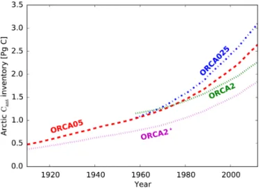
To assess the anthropogenic carbon budget in the Arctic Ocean, we adopt the regional domain defined by Bates and Mathis (2009) delineated in Fig. 1. That domain’s lateral boundaries and the volume of water contained within them vary slightly among the three model versions due to their dif-ferent resolutions and bathymetries (Table 1). The signature of these different volumes is also apparent in the integrated quantity of anthropogenic carbon that is stored in the Arctic in 1958, although the fields for all three models are based on the same 1957 field from the ORCA05 model (Fig. 2).

Figure 2. Arctic Ocean Cant inventory for ORCA2, ORCA05,

ORCA025, and ORCA2∗. The discontinuity for ORCA2 in 1958 is due to its larger total volume of water when integrated across the Arctic domain (Table 1).

2.6 Transport across boundaries

Transects are defined (Fig. 1) along the four boundaries as consistently as possible for the three resolutions. Water trans-port across each of the four boundaries is calculated for each model configuration by using monthly average water veloc-ities at each boundary grid cell along a transect multiplied by the corresponding area of the face of the grid cell through which the water flows. For boundaries defined by a row of cells (Fram Strait; Canadian Arctic Archipelago, CAA; and Bering Strait), the transport is calculated across the north-ern face of each cell. Conversely, for the jagged boundary of the Barents Sea Opening, transport is calculated at the north-ern and eastnorth-ern faces of each cell and the two transports are summed. For each transect, transport across all of its cells is summed to obtain the transect’s monthly net transport.

For the Canttransport, we do the same but also multiply the

water transport at the boundary between two grid cells with their volume-weighted monthly-average concentration. This multiplication of monthly means introduces an error into the transport calculations owing to neglect of shorter-term vari-ability. To elucidate that error, we sum results from those monthly calculations across all four sections, integrate them over time from 1960 to 2012, and compare that to the net transport of Cantinto the Arctic Ocean implied by the

inven-tory change minus the cumulative air–sea flux over the same time period. The inventory of Cantis the total mass of Cant

inside the Arctic Ocean at a given time, while the cumulative flux is the time-integrated air–sea flux of anthropogenic CO2

over the Arctic Ocean since the beginning of the simulation. The difference between these two spatially integrated values is the reference value for the net lateral flux into the Arctic Ocean to which is compared the less exact total lateral flux of anthropogenic carbon computed from monthly mean

veloc-ity and concentration fields integrated over time. The relative error for transport of Cantacross all the separate boundaries

introduced by the monthly average calculations is 28 % for ORCA2, 7 % for ORCA05, and 3 % for ORCA025. This er-ror applies neither to the Cantinventory nor to the cumulative

Cantair–sea flux or the lateral Cantfluxes, which are all

cal-culated online, i.e., during the simulations. 2.7 CFC-12 observational data

Model simulations were evaluated indirectly by comparing simulated to observed CFC-12. We choose CFC-12 to eval-uate the model because it is an anthropogenic, passive, con-servative, and inert tracer, and in contrast to anthropogenic carbon, it is directly measurable. The CFC-12 atmospheric concentration increased from zero in the 1930s to its peak in the 2000s, since declining as a result of the Montreal protocol. Thus, CFC-12 is a transient tracer similar to an-thropogenic carbon but for which there exist extensive direct measurements, all carried out with high precision during the WOCE (World Ocean Circulation Experiment) and CLIVAR (Climate and Ocean – Variability, Predictability and Change) era. Nowadays, ocean models are often evaluated with CFC-11 or CFC-12, especially those used to assess anthropogenic carbon uptake (Dutay et al., 2002; Orr et al., 2017).

The CFC-12 observations used in this study come from two trans-Arctic cruises: the 1994 Arctic Ocean Section (AOS94) (Jones et al., 2007) and the Beringia 2005 expe-dition (Anderson et al., 2011) (Fig. 1). AOS94 started on 24 July and was completed on 1 September, during which CFC-12 measurements were made at 39 stations. That section be-gan in the Bering Strait, entered the Canada Basin adjacent to Mendeleev Ridge, continued to the Makarov Basin, and ended at the boundary of the Nansen Basin and the Barents Sea. The Beringia expedition started on 19 August and ended on 25 September 2005. It began off the coast of Alaska, went through the Canada and Makarov basins and crossed the Lomonosov Ridge, and its last CFC-12 station was taken on the Gakkel Ridge. These two cruises were chosen from among others because they cross large parts of the Arctic, including almost all four major basins.

2.8 Data-based estimates of anthropogenic carbon Our simulated Cant was compared to data-based estimates

from Tanhua et al. (2009) for the year 2005 and from GLO-DAPv2 for the year 2002 (Lauvset et al., 2016), both based on the TTD approach.

3 Results

3.1 Physical evaluation 3.1.1 Lateral water fluxes

The lateral water flux across each of the four Arctic bound-aries is a fundamental reference for the simulated physical transport, especially given our goal to construct a budget that includes the lateral transport of passive tracers. Results for lateral water transport in the three model resolutions may be grouped into two classes: coarse resolution and higher resolutions. In ORCA2, water enters the Arctic Ocean from the Barents Sea and the Bering Strait (2.1 Sv split evenly), with 86 % of that total leaving the Arctic via the Fram Strait and the remaining 14 % flowing out via the CAA (Table 5). Conversely, outflow through the CAA is 7 times larger for ORCA05 and 9 times larger for ORCA025, being fueled by 26 % to 46 % more inflow via the Bering Strait and 110 % to 170 % more inflow via the Barents Sea. Outflow via the Fram Strait is 1.76 Sv in ORCA2, 1.42–1.75 Sv in ORCA05, and 1.46–1.80 Sv in ORCA025, depending on the time pe-riod (Table 5).

Relative to the observed CAA outflow of 2.7 Sv (Curry et al., 2014; Straneo and Saucier, 2008), only ORCA05 and ORCA025 simulate similar results. In contrast, ORCA2’s simulated CAA outflow is about one-ninth of that observed. Likewise, its inflow via the Barents Sea is half of that ob-served, while the two higher-resolution simulations have Barents Sea inflows that are 20 % and 40 % larger than ob-served. Yet for inflow through the Bering Strait, it is ORCA2 that is closest to the observed estimate, overestimating it by 30 %, while ORCA05 and ORCA025 overestimate it by 60 % and 90 %. Thus, too much Pacific water appears to be en-tering the Arctic Ocean. All resolutions underestimate the central observational estimate for the Fram Strait outflow by ∼12 % but still easily fall within the large associated uncer-tainty range.

Summing up, the net water transport across all four bound-aries is not zero. A net Arctic outflow between 0.12 and 0.17 Sv is found for the three model resolutions owing to river inflow and precipitation as well as artifacts caused by using monthly averages. In contrast, when the observed wa-ter transport estimates at all four boundaries are summed up, there is a net outflow of 1.9 Sv, more than 10 times larger. This strong net outflow is also much larger than freshwa-ter input from rivers of 0.08 Sv (McClelland et al., 2006) and precipitation of 0.12 Sv (Yang, 1999). It can only be ex-plained by uncertainties in the data-based estimates of wa-ter transport, which are at least ±2.7 Sv for the net port based on the limited uncertainties available for trans-port across the individual boundaries (Table 5). The exces-sive central observational estimate for the net outflow might be explained by a data-based estimate for the Barents Sea inflow that is too weak combined with a data-based estimate

for the Fram Strait outflow that is too strong, a possibility that is consistent with results from the higher-resolution models ORCA05 and ORCA025.

3.1.2 Sea ice

Because sea-ice cover affects the air–sea CO2flux and hence

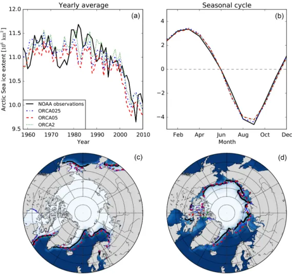
anthropogenic carbon concentrations in the ocean, we com-pare the modeled sea-ice cover to that observed by the US National Snow and Ice Data Center (Walsh et al., 2015). Yearly averages of sea-ice extent agree within 2 % between the observations and models. Only in summer are simu-lated sea-ice concentrations slightly too high (by 0.25–0.5 × 106km3, e.g., 5 %). Despite this overall agreement in inte-grated sea-ice extent, regionally differences are larger. Dur-ing winter (Fig. 3), all three model configurations slightly overestimate the sea-ice extent northeast of Iceland and north of the Labrador Sea, while the simulated sea-ice extent in the Barents Sea and the Bering Strait are similar to observations. During summer, the simulated sea-ice extent resembles that observed in the western Arctic particularly near the Pacific, but all model resolutions slightly overestimate sea-ice extent in the Nordic Seas, north of the Barents Sea, the Kara Sea, and the Laptev Sea. This overestimation should reduce air– sea CO2 fluxes locally in these regions. Overall, the close

model–data agreement for sea-ice extent in terms of the total amount, its trend and seasonal coverage, as well as regional coverage in winter contrasts with the tendency of the models to overpredict sea-ice cover in summer at the highest lati-tudes of the eastern Arctic.

3.1.3 Atlantic water

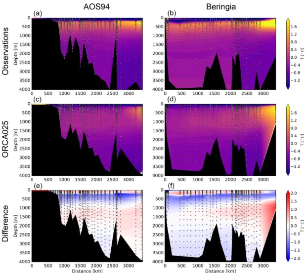
In the Arctic Ocean, water temperature is used to help iden-tify water masses, with values above 0◦C typically coming from the Atlantic Ocean (Woodgate, 2013). The observed temperature along the 1994 and 2005 sections (Fig. 4) in-dicates that Atlantic Water (AW) is found between 200 and 1000 m, penetrating laterally below the strongly stratified Arctic Ocean surface waters. In ORCA025, this AW layer is deeper and more diffuse, lying between 500 and 1500 m and thus leading to a cold bias around 500 m and a warm bias around 1000 m. The Beringia station at the boundary between the Barents Sea and the Nansen Basin indicates that AW lies between 200 m (2.5◦C) and the seafloor at 1000 m (0◦_{C). Conversely in the same location in ORCA025, model}

temperatures remain above 1.5◦_{C throughout the water}

col-umn. That lower maximum temperature and weaker vertical gradient suggest that when ORCA025’s Atlantic water enters the Arctic Ocean through the Barents Sea, it is too diffuse, being well mixed throughout the water column. Weaker max-ima in ORCA025’s simulated temperature relative to obser-vations are also found further west in the Canada Basin along both sections. There, observed temperatures reach maxima

Table 5. Lateral transport of water and Cantacross Arctic Ocean boundaries with average simulated values calculated for the same time

period as observations.

Model configuration Observations Year Sources ORCA2 ORCA05 ORCA025

Lateral water transport (Sv)

Fram Strait −1.76 −1.75 −1.80 −2.0 ± 2.7 1997–2006 Schauer et al. (2008) −1.76 −1.42 −1.46 −1.7 1980–2005 Rudels et al. (2008) Barents Sea 1.20 2.50 2.77 2.0 2003–2005 Skagseth et al. (2008)

1.04 2.42 2.78 2.0 1997–2007 Smedsrud et al. (2010) Bering Strait 1.02 1.29 1.49 0.8 ± 0.2 1991–2007 Woodgate et al. (2010) CAA −0.29 −2.00 −2.59 −2.7 ± 0.2 2004–2013 Curry et al. (2014)

Sum −0.12 −0.16 −0.18

Model configuration Observations Year Sources ORCA2 ORCA05 ORCA025

Lateral Cantfluxes (Tg C yr−1)

Fram Strait −17 −12 −8 −1 ± 17 2002 Jeansson et al. (2011) −17 −7 5 −12 2012 Stöven et al. (2016) Barents Sea 16 43 50 41 ± 8 2002 Jeansson et al. (2011) Bering Strait 18 22 27 18 2000–2010∗ Olsen et al. (2015) CAA −5 −28 −36 −29 2000–2010∗ Olsen et al. (2015) Sum 18 29 38 29 2000–2010∗ Olsen et al. (2015)

∗_{Observational year or period impossible to identify exactly as C}

antand velocity measurements are not from the same year.

of 1.1◦C, while simulated temperature maxima reach only 0.5◦C.

The two lower resolutions represent lateral invasion of AW less successfully than does ORCA025. Both simulations show water with temperatures higher than 0◦C only at the southern end of the Nansen Basin. Vertically, these water masses are situated around 400 m for ORCA2 and between 200 and 1300 m for ORCA05.

3.2 CFC-12

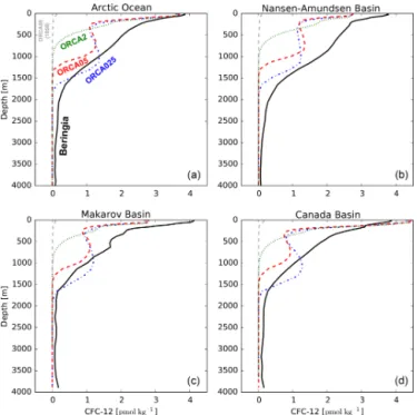
Simulated CFC-12 was compared among the three resolu-tions and with observaresolu-tions, focusing first on basin-scale ten-dencies based on vertical profiles of the distance-weighted means along the Beringia 2005 section (Fig. 5). This compar-ison reveals that among resolutions, simulated CFC-12 con-centrations differ most between 400 and 1900 m; conversely, above and below that intermediate zone, simulated average profiles are nearly insensitive to resolution. In that interme-diate zone and above, simulated concentrations are also gen-erally lower than observed. The only exception is the top 100 m in the Canada Basin where all resolutions overestimate observed concentrations by 10 %. Between 200 and 400 m,

all resolutions underestimate observations by ∼ 50 %. Below 400 m, the ORCA2 CFC-12 concentrations decline quickly to zero by ∼ 1000 m, while the ORCA05 and ORCA025 con-centrations continue to increase, both being 15 % greater at 900 m than at 400 m. Below that depth, the ORCA05 con-centrations decline, quickly reaching zero at 1350 m, while ORCA025 concentrations remain above 1 pmol kg−1 until 1400 m. Between 1100 and 1500 m, average CFC-12 con-centrations along the Beringia section in ORCA025 are up to ∼10 % larger than observed. This overestimation of CFC-12 by ORCA025 reaches up to 40 % in the Canada and Makarov basins. Below 1900 m, the simulated concentra-tions are essentially zero, while the observaconcentra-tions are slightly higher (0.12 pmol kg−1). For comparison, the reported de-tection limit for CFC-12 for the Beringia 2005 expedition is 0.02 pmol kg−1(Anderson et al., 2011).

Given the closer overall agreement of the ORCA025 sim-ulated CFC-12 to the observations, let us now focus on its evaluation along the 1994 and 2005 sections (Fig. 6). On the Atlantic end of the Beringia 2005 section, where water enters the Nansen Basin from the Barents Sea, the water column in ORCA025 appears too well mixed, having CFC-12 con-centrations that remain above 2.0 pmol kg−1. Conversely,

ob-Figure 3. Sea-ice extent (a, b) and sea-ice concentration (c, d) over the Arctic from 1960 to 2012 comparing microwave-based observations from the National Oceanic and Atmospheric Administration (NOAA) (black) to simulated results from ORCA2 (green dots), ORCA05 (red dashes), and ORCA025 (blue dot–dash). Shown are the yearly averages (a), the average (climatological) seasonal cycle over 1958–2010 (b), and the average sea-ice extent in winter (December, January, February) (c) and summer (July, August, September) (d). The lines on the maps show the 50 % sea-ice cover for the three model resolutions and the observations, while the color indicates the observed sea-ice concentration.

served CFC-12 is less uniform, varying from 2.8 pmol kg−1 at the surface to 1.3 pmol kg−1in bottom waters at 1000 m, thereby indicating greater stratification. A similar contrast in stratification was deduced from modeled and observed tem-perature profiles at the same location (Sect. 3.1.3). On the other side of the Arctic in the Canada Basin, there are ob-served local chimneys of CFC-12 where concentrations re-main at about 2.0 pmol kg−1from near the surface down to 1000 m, particularly along the 1994 section. These chim-neys suggest localized mixing that is only barely apparent in ORCA025 (Fig. 6). Such localized features are absent at lower resolution. The CFC-12 inventories were also calcu-lated along the two sections, integrated over depth and dis-tance (Table 7). Depending on the expedition, ORCA025 underestimates the observed CFC-12 section inventories by 13 %–18 %, ORCA05 by 36 %–38 %, and ORCA2 by 47 %– 61 %.

3.3 Anthropogenic carbon inventories and concentrations

Simulated global ocean Cant inventories are 152 Pg C in

ORCA2, 146 Pg C in ORCA05, and 148 Pg C in ORCA025 in 2008, after accounting for corrections for the earlier start-ing date of 1765 usstart-ing our perturbation simulations (P1765– P1870). The correction is similar for each resolution, e.g., 24–25 Pg C in 1995, and is consistent with our biogeochem-ical model simulation strategy (all three resolutions initial-ized with the ORCA05 output in 1958). Furthermore, these model-based corrections fall within the 29 ± 5 Pg C correc-tion calculated for the same 1765–1995 period with a data-based approach (Bronselaer et al., 2017). For the 1765–2008 period, the data-based global Cant inventory estimate from

(Khatiwala et al., 2009) is 140 ± 24 Pg C, the range of which encompasses the results from all three model resolutions.

In the Arctic Ocean, the corrected modeled Cant

Figure 4. Temperature along the 1994 Arctic Ocean Section (AOS94) cruise (a, c, e) and the Beringia 2005 section (b, d, f), both trans-Arctic transects (Fig. 1). The observations (a, b) are compared to simulated results from ORCA025 averaged over the summer of the respective year (c, d). The model–data difference is shown at the bottom.

2.6 Pg C in 2005, in each case with the low from ORCA2 and the high from ORCA025 (Table 6 and Fig. 2). These sim-ulated basin-wide Arctic Ocean Cant inventories were

com-pared to the TTD-based estimates of anthropogenic carbon from (1) the GLODAPv2 assessment (Lauvset et al., 2016) normalized to the year 2002 and (2) the Tanhua et al. (2009) assessment normalized to 2005. The data-based assessment from GLODAPv2 suggests that 2.9 Pg C of anthropogenic carbon was stored in the Arctic Ocean in 2002, while that from Tanhua et al. (2009) suggests that 2.5–3.3 Pg C was stored there in 2005. In 2002, the upper limit of the mod-eled Cant inventory range remains 0.4 Pg C lower than the

GLODAPv2 data-based estimate, but the ORCA025 result in 2005 falls within the data-based uncertainty range of Tanhua et al. (2009). As for the global estimates, the modeled Arctic Ocean Cantinventories include corrections for the late

start-ing date of the biogeochemical simulations. This correction is 0.4 Pg C in 2005 for each of the three resolutions (Table 6).

The differences in basin-wide inventory estimates were further studied by comparing vertical profiles of Cant from

the models to those from the GLODAPv2 data-based es-timates (Fig. 7). Surface concentrations in ORCA05 and ORCA025 are up to ∼ 35 % larger (+12 µmol kg−1) than the data-based estimate, whereas the ORCA2 concentration is ∼22 % larger (+7 µmol kg−1). By 150 m, the simulated con-centrations in all resolutions have dropped below the data-based estimates and remain so, except for ORCA025, down to the ocean bottom. Data–model differences are largest at 400 m, with all resolutions underestimating data-based Cant estimates by up to ∼ 28 % (9 µmol kg−1). Below that

depth, results from the three resolutions differ more. The Cant

concentration in ORCA2 decreases monotonically reaching 11 µmol kg−1at 1000 m and essentially zero by 2300 m. The vertical penetration of Cantin ORCA2∗(the simulation

with-out branching from ORCA05 in 1958) is shallower, reach-ing zero by 1400 m. In ORCA05, Cant concentrations

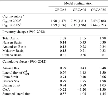
Table 6. Total inventory, its change during 1960–2012, the cumulative air–sea flux, and the lateral flux of Cantin Pg C.

Model configuration

ORCA2 ORCA05 ORCA025 Cantinventorya Cantin 2002b 1.90 (1.47) 2.25 (1.81) 2.49 (2.06) Cantin 2005c 1.99 (1.56) 2.37 (1.96) 2.64 (2.21) Inventory change (1960–2012) Total Arctic 1.08 1.55 1.98 Nansen Basin 0.14 0.33 0.30 Amundsen Basin 0.13 0.28 0.34 Makarov Basin 0.15 0.21 0.33 Canada Basin 0.31 0.36 0.61 Cumulative fluxes (1960–2012) Air–sea flux 0.29 0.43 0.48 Lateral flux of Cd_ant 0.79 1.13 1.50 Fram Strait −0.74 −0.40 −0.06 Barents Sea 0.79 1.75 1.98 Bering Strait 0.74 0.89 1.03

CAA −0.22 −1.20 −1.50

Summed lateral flux 0.57 1.05 1.45

a_{Numbers in parentheses show the uncorrected value (starting date 1870).}b_{Data-based inventory}

in 2002: 2.95 Pg C (GLODAPv2).c_{Data-based inventory in 2005: 3.03 Pg C (2.5–3.3) (Tanhua}

et al., 2009).d_{Computed as inventory change minus cumulative air–sea flux.}

Table 7. Along-section CFC-12 inventories (µmol m−1) integrated over depth and distance along the AOS94 and Beringia 2005 sec-tions vs. colocated results in ORCA2, ORCA05, and ORCA025.

AOS94 Beringia 2005 Observation 5.5 9.4

ORCA2 2.9 3.7

ORCA05 3.5 5.8

ORCA025 4.8 7.7

decline rapidly, reaching zero at 2300 m. Only in ORCA025 do Cant concentrations increase again below 400 m,

reach-ing a local maximum at 900 m, an increase that causes the ORCA025 results to exceed data-based estimates by up to 2 µmol kg−1 (∼ 11 %) at 1100 m. A similar maximum and excess are also seen in the CFC-12 profile for ORCA025 as is the minimum around 400 m (Fig. 5). Below 1500 m, the ORCA025 Cant concentrations decline quickly,

essen-tially reaching zero at 2300 m. Conversely, data-based Cant

concentrations remain roughly constant at 6 µmol kg−1down to the seafloor. Thus, the largest vertically integrated differ-ences between ORCA025 and data-based estimates are found in the deep Arctic Ocean below 1600 m.

3.4 Anthropogenic carbon budget

For the budget of Cant, we focused on the final decades over

which the model resolutions differed (Tables 5 and 6). Dur-ing 1960 to 2012, the Cantinventory in ORCA025 increased

by 1.98 Pg C, 80 % of which is stored in the four major Arc-tic Ocean basins: the Nansen Basin (0.30 Pg C), the Amund-sen Basin (0.34 Pg C), the Makarov Basin (0.33 Pg C), and the Canada Basin (0.61 Pg C). Although the Canada Basin Cantinventory increased most, its volume is larger so that its

average Cant concentration increased less than in the other

basins (Fig. 7). Of the total inventory stored in the Arctic Ocean during that time, only about one-fourth (0.48 Pg C) entered the Arctic Ocean via the air–sea flux, most of which was transferred from the atmosphere through the surface of the Barents Sea (Fig. 8). The remaining 75 % (1.50 Pg C) entered the Arctic Ocean via lateral transport. This net lat-eral influx is the sum of the fluxes (1) from the Atlantic to the Barents Sea (1.98 Pg C), (2) from the Pacific through the Bering Strait (1.03 Pg C), (3) to the Atlantic via the Fram Strait (−0.06 Pg C), and (4) to the Atlantic via the CAA (−1.50 Pg C). Summed up, the net lateral inflow of anthro-pogenic carbon across the four boundaries is 1.45 Pg C. This lateral flux computed from monthly mean Cant

concentra-tions and flow fields is 0.05 Pg C (∼ 3 %) smaller than the lateral flux computed from the change in inventory minus the cumulative air–sea flux (Fig. 8). Within the Arctic, coastal

Figure 5. Profiles of observed CFC-12 (black solid) and simu-lated CFC-12 in ORCA2 (green dots), ORCA05 (red dashes), and ORCA025 (blue dot–dash) along the Beringia 2005 section. Shown are distance-weighted means across that entire section (a) as well as over that section covering the Nansen and Amundsen basins (b), the Makarov Basin (c), and the Canada Basin (d). Shown in light grey is the vertical profile in 1958, the branching point for the three resolutions.

regions typically exhibit net lateral losses, while the deep basins exhibit net lateral gain. The largest lateral loss occurs in the Barents Sea, where the cumulative air–sea flux of Cant

is also largest.

The budget of Cant changes notably with resolution.

Higher resolution results in more simulated Cantbeing stored

in the Arctic region, with increases in both the cumula-tive air–sea flux and lateral transport. The Cant inventory

change from 1960 to 2012 nearly doubles with the resolu-tion increase between ORCA2 and ORCA025 (from 1.08 to 1.98 Pg C). Of that additional Cant, 93 % is found

be-tween 300 and 2200 m, with the maximum being located at 1140 m. The remaining 7 % is located in the upper 300 m (Fig. 7). Resolution also affects the regional partitioning of Cant(Figs. 7 and 8). When refining resolution from ORCA2

to ORCA05, the Arctic Ocean Cant inventory increases by

0.47 Pg C, 72 % of which occurs in the Eurasian basins: the Nansen Basin (0.19 Pg C) and Amundsen Basin (0.15 Pg C). Another 23 % of that increase occurs in the Amerasian basins: the Makarov Basin (0.06 Pg C) and Canada Basin (0.05 Pg C). Coastal regions account for only 5 % of the total inventory increase. In contrast, the subsequent resolution en-hancement between ORCA05 and ORCA025 results in little

increase in inventory in the Eurasian basins (0.03 Pg C) but much more in the Amerasian basins (0.37 Pg C).

As resolution is refined between ORCA2 and ORCA025, the Arctic Cantinventory increases as a result of a 66 %

in-crease in the air–sea flux (+0.19 Pg C) and a 90 % inin-crease in the lateral flux (+0.71 Pg C). Thus, the relative contribu-tion of the lateral flux increases from 73 % to 76 %. Changing model resolution also affects the pathways by which Cant

en-ters the Arctic Ocean (Table 5). The most prominent change occurs in the CAA. From ORCA2 to ORCA025, the net out-flow of Cantthrough the CAA increases 7-fold (from −0.22

to −1.50 Pg C). Other notable changes include (1) the net outflow through the Fram Strait declining 12fold from -0.74 to −0.06 Pg C, (2) the inflow through the Barents Sea increasing by 150 % (from 0.79 to 1.98 Pg C), and (3) the inflow of Cant through the Bering Strait increasing by 39 %

(from 0.74 to 1.03 Pg C).

4 Discussion 4.1 CFC-12

The simulated CFC-12 in ORCA025 underestimates ob-served concentrations between 100 and 1100 m, slightly overestimates them on average between 1100 and 1500 m, and again underestimates the low observed concentrations below 1500 m. The temperature sections suggest that ex-cess simulated CFC-12 between 1100 and 1500 m is due to a vertical displacement of inflowing Atlantic water, which descends too deeply into the Arctic (Fig. 4). Such vertical displacement would indeed reduce simulated CFC-12 con-centrations above 1000 m and enhance them between 1100 and 1500 m. Yet the underestimation of integrated CFC-12 mass above 1100 m is larger than the overestimation below 1100 m. Thus, vertical displacement of Atlantic water cannot provide a full explanation. Simulated CFC-12 concentrations above 1100 m could also be too low because ventilation of subsurface waters is too weak, a hypothesis that is consistent with the simulated vertical gradients in both temperature and CFC-12 that are too strong between 100 and 1100 m. 4.2 Anthropogenic carbon

Vertical profiles of Cant and CFC-12 are similar. Above

1000 m, ORCA025 underestimates data-based estimates of Cant as well as observed CFC-12 owing to weak

ventila-tion in the model. Between 1000 and 1500 m, simulated Cant

and CFC-12 in ORCA025 exhibit local maxima, which make them on average slightly higher than data-based and ob-served concentrations. These local maxima can be explained by the simulated Atlantic water masses, rich in both trac-ers, being too deep. However, the slight overestimation be-tween 1000 and 1500 m is much smaller than the underesti-mation between 200 and 1000 m. Below 2000 m, simulated Cant largely underestimates data-based estimates. The low

Figure 6. CFC-12 concentrations along the AOS94 section (a, c, e) and the Beringia section (b, d, f) for the observations (a, b), the simulated summer means in ORCA025 (c, d), and the model–data difference (e, f).

simulated Cantstems from too little deep-water formation in

the model as indicated by the absence of simulated CFC-12 below 2000 m, an absence that contrasts with the observed CFC-12 concentrations that remain detectable all the way down to the ocean floor (Fig. 5).

A second reason for the low simulated Arctic Cant

inven-tory in ORCA025 is that it was initialized with ORCA05 results in 1958. Had ORCA025 been initialized in 1765, which was not computationally feasible, its simulated inven-tory would be larger, given that both Cantand CFC-12

stor-age for ORCA025 are larger than those for ORCA05 over 1958–2012. That hypothesis is consistent with our finding that ORCA2∗ (complete simulation at 2◦ without branch-ing from the 0.5◦ configuration) takes up less Cant than

does ORCA2 (0.5◦until 1958 then 2◦afterwards), which is in line with ORCA2 taking up less Cant and CFC-12 than

ORCA05 (Figs. 2, 5, and 7). The initialization of ORCA2 with ORCA05 output in 1958 mainly affects Cantstorage

be-tween 1000 and 2000 m, the same depth range over which differences in simulated CFC-12 concentrations are largest

between ORCA2 and ORCA05. Nevertheless, that 1958 ini-tialization has little effect on subsequent changes in Cant

stor-age, cumulative lateral flux, and air–sea flux (Fig. 9). Rather it is the changes before 1958 that dominate the difference between ORCA2 and ORCA2∗.

All our model configurations underestimate Cant

concen-trations in the deep waters of the Arctic Ocean based on the CFC-12 model evaluation. The same conclusion is drawn from comparing simulated to data-based estimates of Cant.

However, results from different data-based approaches to es-timate Cant can differ substantially in the deep ocean (e.g.,

Vázquez-Rodríguez et al., 2009). Furthermore, the TTD ap-proach typically produces the highest values in deep wa-ters due to its assumption of constant air–sea disequilibrium (Khatiwala et al., 2013). Hence applying other data-based ap-proaches to assess the Arctic Ocean inventory of the Cant

in-ventory would eventually help to further constrain uncertain-ties.

Figure 7. Area-weighted basin-wide average vertical profiles of Cant concentration in 2002 for GLODAPv2 data-based estimates

(black solid), ORCA2 (green dots), ORCA05 (red dashes), and ORCA025 (blue dot–dash) over the entire Arctic (a) as well as over the Nansen and Amundsen basins (b), the Makarov Basin (c), and the Canada Basin (d). Ocean corrected for the starting year by the perturbation approach simulations. Shown are the vertical profile in 1958 (dashed, light grey), the branching point for the three resolu-tions, and results from ORCA2∗for 2002 (magenta dots).

4.3 Lateral flux

In our model, about three-fourths of the net total mass of Cant

that accumulates in the Arctic Ocean enters laterally from the Atlantic and Pacific oceans, independent of model resolution. Our simulated lateral fluxes of Cantin ORCA025 were

com-pared to based estimates from studies that multiply data-based Cantconcentrations (TTD estimates) along the Arctic

boundaries by corresponding observation-based estimates of water transport.

The simulated lateral transport of Cantin ORCA025

gen-erally agrees with data-based estimates within their large un-certainties. These uncertainties result from uncertainties in data-based estimates of Cantand from uncertainties in

obser-vational constraints on water flow, which also varies interan-nually (Jeansson et al., 2011). For the Fram Strait, Jeansson et al. (2011) estimated a net Cantoutflux (from the Arctic) of

1 ± 17 Tg C yr−1in 2002, while for 2012 Stöven et al. (2016) estimate an outflux of 12 Tg C yr−1 without indicating un-certainties. For the same years, ORCA025 simulates a net outflux of 8 Tg C yr−1in 2002 but a net influx (to the Arctic) of 5 Tg C yr−1in 2012. Both model and data-based estimates vary greatly between 2002 and 2012. Across the Barents Sea

Opening, there is a consistent net influx from the Atlantic to the Arctic Ocean, i.e., 41 ± 8 Tg C yr−1in 2002 for the data-based estimate (Jeansson et al., 2011) and 50 Tg C yr−1 for ORCA025 in the same year.

More recently, Olsen et al. (2015) added data-based es-timates of lateral fluxes of Cant across the two other major

Arctic Ocean boundaries, completing the set of four bound-aries that define the perimeter. They estimate a Cant influx

of ∼18 Tg C yr−1from the Pacific through the Bering Strait and a Cantoutflux through the CAA of ∼ 29 Tg C yr−1, both

for the 2000s. For the same time period, ORCA025 simulates 50 % more inflow through the Bering Strait (∼ 27 Tg C yr−1) and 24 % more outflow through the CAA (∼ 36 Tg C yr−1). The larger Bering Strait Cantinflux in ORCA025 is

consis-tent with its overestimated Bering Strait water inflow (Ta-ble 5, Sect. 3.1.1). Integrating over all four lateral bound-aries, Olsen et al. (2015) found a total net Cant influx

of ∼ 29 Tg C yr−1, which is 24 % less than that simulated in ORCA025 averaged over 2000–2010 (∼ 38 Tg C yr−1). Olsen et al. (2015) did not provide uncertainties, but the uncertainty of their net lateral flux estimate is at least ±18 Tg C yr−1 based on the data-based transport estimates at the two other Arctic boundary sections where uncertain-ties are available (Table 5).

Weighing in at about one-fourth of the lateral flux is the simulated air–sea flux of Cantin ORCA025 of 10 Tg C yr−1

when both are averaged over 2000–2010. That simulated estimate is only about 40 % of the data-based estimate of 26 Tg C yr−1 from Olsen et al. (2015). Although no uncer-tainty is provided with that data-based air–sea flux estimate, it too must be at least ±18 Tg C yr−1given that it is calcu-lated as the difference between the data-based storage esti-mate (Tanhua et al., 2009) and the Olsen et al. (2015) data-based net lateral flux. The simulated air–sea flux of Cantfalls

within that assigned uncertainty range for the data-based es-timate. In any case, both the model and data-based estimates suggest that the air–sea flux of Cantis not the dominant

con-tributor to the anthropogenic carbon budget of the Arctic Ocean, respectively representing 21 % and 47 % of the to-tal Cantinput averaged over 2000–2010. For both, the lateral

flux dominates. 4.4 Model resolution

Basin inventories of simulated anthropogenic carbon differ between model configurations because of how resolution affects their volume, bathymetry, circulation patterns, and source waters. Much of the water in the Nansen and Amund-sen basins has entered laterally from the Atlantic Ocean through the Fram Strait and the Barents Sea (Jones et al., 1995). Water inflow through the Barents Sea increases by 150 % when moving from ORCA2 to ORCA05 but only by 20 % more between ORCA05 and ORCA025. Water inflow in those two higher-resolution models is also closer to obser-vational estimates. Along with the increase in water inflow,

Figure 8. Inventory change (a, d, g), cumulative air–sea flux (b, e, h), and the lateral flux calculated as the inventory change minus the cumulative air–sea flux (c, f, i) of Cantover 1960–2012 for ORCA025 (a–c), ORCA05 (d–f), and ORCA2 (g–i).

Figure 9. Comparison of results for the Arctic Ocean from ORCA2, ORCA05, ORCA025, and ORCA2∗and the nine earth system models that participated in CMIP5. Shown are the Cantinventory in 2005 (black), the inventory change of Cant(dark grey) between 1960 and 2012,

the corresponding cumulative air–sea flux of Cant(light grey), and the cumulative lateral flux of Cant(white). Also indicated are the

data-based estimate from Tanhua et al. (2009) (dashed black line) along with its associated uncertainty range (grey background). The inventory correction for the late starting date for our forced simulations is indicated as striped bars.

higher resolution also increases the lateral influx of Cant. Yet

despite this increase in the Cant lateral influx, the air–sea

Cantflux into the Arctic Ocean also increases with resolution.

This finding can be explained by two mechanisms:(1) higher resolution decreases the outflux of Cant through the Fram

Strait, which mainly occurs in subsurface currents and thus does not greatly affect surface Cant concentrations nor air–

sea exchanges of Cant, and (2) higher resolution enhances

deep-water formation, mainly in the Barents Sea, which re-duces surface Cant and thus enhances the air-to-sea flux of

Cant. Although the air–sea flux of Cantincreases slightly, the

larger lateral water fluxes in ORCA05 and ORCA025 mainly explain their higher Cant concentrations in the Nansen and

Amundsen basins. Some of this inflowing water continues to flow further along the slope, across the Lomonosov Ridge into the Makarov Basin, and then across the Mendeleev Ridge into the Canada Basin. Yet how well models simu-late that flow path depends on simu-lateral resolution. Between ORCA2 and ORCA05, Cantinventories increase by 16 % in

the Canada Basin (+0.05 Pg C) and by 40 % the Makarov Basin (+0.06 Pg C). But between ORCA05 and ORCA025, increases are 2 to 5 times greater: +0.25 Pg C in the Canada Basin and +0.12 Pg C in the Makarov Basin (Sect. 3.4). The change from ORCA2 to ORCA05 mainly seems to improve lateral exchanges with adjacent oceans, while the change from ORCA05 to ORCA025 improves interior Arctic Ocean circulation.

As the increase from ORCA05 to ORCA025 stems from a finer, more realistic representation of lateral transport within the Arctic, it would appear that eddying ocean models may be needed to adequately simulate the interior circulation in terms of its effect on Cantstorage in the Arctic Ocean. In the

Canada Basin, such lateral inflow may not be the only source of Cant. Another major source appears to come from density

flows along the continental slope, driven by brine rejection from sea-ice formation over the continental shelves (Jones et al., 1995). A signature of this source in the observed sec-tions may be the chimneys of constant CFC-12 concentration from the surface to about 1000 m in the Canada Basin, fea-tures for which only ORCA025 exhibits any such indication, albeit faint. To adequately model lateral exchanges of Cant

in the Arctic Ocean, at least a resolution comparable to that used in ORCA05 may be needed, while resolutions compa-rable to that in ORCA025 or above may well be required to begin to capture the effects from density flows along the slope. As a consequence of the deficient representation of these density flows, we would expect to see an increase in Cantwhen using even higher resolution.

Improved modeled circulation from higher model resolu-tion has also been shown to be critical to improving simu-lated anthropogenic tracers in the Southern Ocean (Lachkar et al., 2007) and simulated oxygen concentrations in the trop-ical Atlantic (Duteil et al., 2014).

4.5 CMIP5 comparison

For a wider perspective, we compared results from our forced NEMO-PISCES simulations to those from nine ocean bio-geochemical models that were coupled within different earth system modeling frameworks as part of CMIP5 (Table 8, Fig. 9). When the CMIP5 models are compared to the data-based estimate of the Cantinventory, only the MIROC-ESM

with its inventory of 2.7 Pg C falls within the data-based un-certainty estimate (2.5 to 3.3 Pg C in 2005). The next closest CMIP5 models are NorESM1-ME and HadGEM2-ES, which fall below the lower limit of the data-based range by 0.1 and 0.5 Pg C. Then come the MPI-ESM and GFDL-ESM models with their Cant inventories in 2005 that are 0.9 to 1.5 Pg C

lower than the lower limit. The lowest CMIP5 estimates are from both versions of the IPSL model, whose inventories reach only ∼ 20 % of the data-based range. Adjusting all the CMIP5-model Arctic inventories upward by ∼ 0.4 Pg C to account for their late start date in 1850, as we did for our three simulations, would place two of them (MIROC-ESM and Nor(MIROC-ESM1-ME) above the lower boundary of the data-based uncertainty estimate and another (HadGEM2-ES) just 0.1 Pg C below this lower boundary. Lateral fluxes over 1958–2012 also vary between CMIP5 models from an out-flow of 0.3 Pg C in the IPSL-CM5A-LR model to an inout-flow of 1.1 Pg C in the MIROC-ESM model. Only the first three CMIP5 models mentioned above exhibit large net inflow of Cantinto the Arctic Basin (between 0.7 and 1.1 Pg C during

1960–2012), a condition that appears necessary to allow a model to approach the estimated data-based inventory range. Indeed, the six other CMIP5 models have lower lateral fluxes (−0.5 to 0.5 Pg C) and simulate low Cantstorage in 2005.

What is perhaps most surprising are the large differences between our forced ORCA2∗ model and the IPSL-CM5A-LR and IPSL-CM5A-MR ESMs. All three of those models use the same coarse-resolution ocean model, although both ESMs rely on an earlier version with a different vertical res-olution (31 instead of 46 vertical levels). The contrast in ver-tical resolution may explain part of the large difference in inventories (1.3 Pg C for our forced version that is not cor-rected for the late starting date vs. 0.3–0.6 Pg C for the two coupled versions) but the forcing could also play a role. Lat-eral resolution is not the only factor when aiming to provide realistic simulations of Cant storage and lateral transport in

the Arctic. Sensitivity studies testing other potentially criti-cal factors are merited.

Table 8. CMIP5 models used in this study and the corresponding model groups.

Model name Modeling center

IPSL-CM5A-LR Institut Pierre-Simon Laplace (IPSL) IPSL-CM5A-MR

GFDL-ESM2G NOAA Geophysical Fluid Dynamics Laboratory (NOAA GFDL) GFDL-ESM2M

MPI-ESM-MR Max-Planck-Institut für Meteorologie (Max Planck Institute for Meteorology) MPI-ESM-LR

HadGEM2-ES Met Office Hadley Centre (additional HadGEM2-ES realizations contributed by Instituto Nacional de Pesquisas Espaciais)

MIROC-ESM Japan Agency for Marine-Earth Science and Technology, Atmosphere and Ocean Research Institute (The University of Tokyo), and National Institute for Environmental Studies

NorESM1-ME Norwegian Climate Centre

Figure 10. Profiles of A for ORCA05 in 1960 (black solid) as

well as ORCA2 (green dots), ORCA05 (red dashes), and ORCA025 (blue dot–dash) in 2012. The vertical black dashed line indicates the chemical threshold where A=1. The point where that vertical

line intersects the other curves indicates the depth of the ASH.

4.6 Effect on aragonite saturation state

Given that simulated Cantis affected by lateral model

resolu-tion, so must be simulated ocean acidification. The aragonite saturation state (A) was computed for each resolution from

the historical run’s CT, AT, T , S, PT, and SiT, after

correct-ing CTand ATfor drift based on the control run. The higher

concentrations of Cantin the ORCA05 and ORCA025

sim-ulations reduces A between 1960 and 2012 by more than

twice as much as found with ORCA2 during the same period (Fig. 10). These differences translate into different rates of shoaling for the aragonite saturation horizon (ASH), i.e., the depth where A=1. During 1960–2012, the ASH shoals by

∼50 m in ORCA2, while it shoals by ∼150 m in ORCA05 and ∼ 210 m in ORCA025. Thus, model resolution also af-fects the time at which waters become undersaturated with

respect to aragonite with higher resolution producing greater shoaling.

Although basin-wide mean surface A does not differ

among resolutions, there are regional differences such as over the Siberian Shelf (Fig. 11). The minimum A in

that region reaches 0.9 in ORCA2, while it drops to 0.3 in ORCA05 and 0.1 in ORCA025. That lower value in ORCA025 is more like that observed, e.g., down to 0.01 in the Laptev Sea (Semiletov et al., 2016). As these lows in A

are extremely local, they cannot be expected to be captured in coarse-resolution models such as ORCA2. Higher-resolution models are needed in the Arctic to assess local extremes not only in terms of ocean acidification but also other biogeo-chemical variables.

5 Conclusions

Global-ocean biogeochemical model simulations typically have coarse resolution and tend to underestimate the mass of Cantstored in the Arctic Ocean. Our sensitivity tests suggest

that more realistic results are offered by higher-resolution model configurations that begin to explicitly resolve ocean eddies. Our high-resolution model simulates an Arctic Cant

inventory of 2.6 Pg C in 2005, falling within the uncertainty from the data-based estimates (2.5–3.3 Pg C). That model es-timate should be considered a lower bound because it gen-erally underestimates CFC-12 concentrations. Thus, it sentially confirms the lower bound from the data-based es-timates, which are based on CFC-12-derived Cant

concen-trations that are not without uncertainties, particularly in the deep Arctic Ocean where measured CFC-12 concentra-tions are small. The high-resolution model would have sim-ulated a higher Arctic Cant inventory had computational

re-sources been available to use it throughout the entire indus-trial era rather than initializing it in 1958 with results from