Global model simulations of the impact of ocean-going ships on aerosols, clouds, and the radiation budget

(1)

HAL Id: hal-00302931

https://hal.archives-ouvertes.fr/hal-00302931

Submitted on 2 Jul 2007

HAL is a multi-disciplinary open access

archive for the deposit and dissemination of sci-entific research documents, whether they are pub-lished or not. The documents may come from teaching and research institutions in France or abroad, or from public or private research centers.

L’archive ouverte pluridisciplinaire HAL, est destinée au dépôt et à la diffusion de documents scientifiques de niveau recherche, publiés ou non, émanant des établissements d’enseignement et de recherche français ou étrangers, des laboratoires publics ou privés.

Global model simulations of the impact of ocean-going

ships on aerosols, clouds, and the radiation budget

A. Lauer, V. Eyring, J. Hendricks, P. Jöckel, U. Lohmann

To cite this version:

A. Lauer, V. Eyring, J. Hendricks, P. Jöckel, U. Lohmann. Global model simulations of the impact of ocean-going ships on aerosols, clouds, and the radiation budget. Atmospheric Chemistry and Physics Discussions, European Geosciences Union, 2007, 7 (4), pp.9419-9464. �hal-00302931�

(2)

ACPD

7, 9419–9464, 2007 The impact of emissions from ocean-going ships A. Lauer et al. Title Page Abstract Introduction Conclusions References Tables Figures ◭ ◮ ◭ ◮ Back Close

Full Screen / Esc

Printer-friendly Version Interactive Discussion

EGU

Atmos. Chem. Phys. Discuss., 7, 9419–9464, 2007 www.atmos-chem-phys-discuss.net/7/9419/2007/ © Author(s) 2007. This work is licensed

under a Creative Commons License.

Atmospheric Chemistry and Physics Discussions

Global model simulations of the impact of

ocean-going ships on aerosols, clouds,

and the radiation budget

A. Lauer1, V. Eyring1, J. Hendricks1, P. J ¨ockel2, and U. Lohmann3

1

DLR-Institut f ¨ur Physik der Atmosph ¨are, Oberpfaffenhofen, Germany

2

Max Planck Institute for Chemistry, Mainz, Germany

3

Institute of Atmospheric and Climate Science, Zurich, Switzerland

Received: 11 June 2007 – Accepted: 20 June 2007 – Published: 2 July 2007 Correspondence to: A. Lauer (axel.lauer@dlr.de)

(3)

ACPD

Full Screen / Esc

EGU

Abstract

International shipping contributes significantly to the fuel consumption of all transport related activities. Specific emissions of pollutants such as sulfur dioxide (SO₂) per kg of fuel emitted are higher than for road transport or aviation. Besides gaseous pollutants, ships also emit various types of particulate matter. The aerosol impacts the Earth’s

5

radiation budget directly by scattering and absorbing incoming solar radiation and indi-rectly by changing cloud properties. Here we use ECHAM5/MESSy1-MADE, a global climate model with detailed aerosol and cloud microphysics, to show that emissions from ships significantly increase the cloud droplet number concentration of low mar-itime water clouds. Whereas the cloud liquid water content remains nearly unchanged

10

in these simulations, effective radii of cloud droplets decrease, leading to cloud optical thickness increase up to 5–10%. The sensitivity of the results is estimated by using three different emission inventories for present day conditions. The sensitivity analysis reveals that shipping contributes with 2.3% to 3.6% to the total sulfate burden and 0.4% to 1.4% to the total black carbon burden in the year 2000. In addition to changes in

15

aerosol chemical composition, shipping increases the aerosol number concentration, e.g. up to 25% in the size range of the accumulation mode (typically >0.1 µm) over the Atlantic. The total aerosol optical thickness over the Indian Ocean, the Gulf of Mexico and the Northeastern Pacific increases up to 8–10% depending on the emission inven-tory. Changes in aerosol optical thickness caused by the shipping induced modification

20

of aerosol particle number concentration and chemical composition lead to a change of the net top of the atmosphere (ToA) clear sky radiation of about −0.013 W/m2 to −0.036 W/m2 on global annual average. The estimated all-sky direct aerosol effect calculated from these changes ranges between −0.009 W/m2 and −0.014 W/m2. The indirect aerosol effect of ships on climate is found to be far larger than previously

esti-25

mated. An indirect radiative effect of −0.19 W/m2 to −0.6 W/m2 (change of the top of the atmosphere shortwave radiative flux) is calculated here, contributing 17% to 39% to the total indirect effect of anthropogenic aerosols. This contribution is high because

(4)

ACPD

Full Screen / Esc

EGU

ship emissions are released in regions with frequent low marine clouds in an other-wise clean environment. In addition, the potential impact of particulate matter on the radiation budget is larger over the dark ocean surface than over polluted regions over land.

1 Introduction 5

Besides gaseous pollutants such as nitrogen oxides (NO_x=NO+NO2), carbon

monox-ide (CO) or sulfur dioxmonox-ide (SO₂), ships also emit various types of particulate matter (Eyring et al., 2005a). Due to low restrictive regulations for international shipping and the use of low quality fuel by most ocean-going ships, shipping contributes for example to around 8% to the present total anthropogenic SO₂emissions (Olivier et al., 2005).

10

The aerosol impacts the Earth’s radiation budget directly by scattering and absorbing incoming solar radiation and indirectly by changing cloud properties. Aerosols emitted by ships can be an additional source of cloud condensation nuclei (CCN) and thus pos-sibly result in a higher cloud droplet concentration (Twomey et al., 1968). The increase in cloud droplet number concentration can lead to an increased cloud reflectivity, known

15

as indirect aerosol effect. Measurements in the Monterey Ship Track Experiment con-firmed this hypothesis (Durkee et al., 2000; Hobbs et al., 2000). This mechanism can also cause anomalous cloud lines, so-called ship tracks, which have often been ob-served in satellite data (e.g. Schreier et al., 2006, 20071). In addition, aerosols from shipping might also change cloud cover and precipitation formation efficiency as well

20

as the average cloud lifetime.

Although a rapid growth of the world sea trade and hence increased emissions from international shipping are expected in the future (Eyring et al., 2005b), the potential global influence of aerosols from shipping on atmosphere and climate has received

lit-1

Schreier, M., Mannstein, H., Eyring, V., and Bovensmann, H.: Global ship track distribution and radiative forcing from 1-year of AATSR-data, Geophys. Res. Lett., submitted, 2007.

(5)

ACPD

Full Screen / Esc

EGU

tle attention so far. Available studies on the global impact of ship emissions on climate concentrate on greenhouse gases such as carbon dioxide (CO₂), methane (CH₄) or ozone (O₃) as well as the direct effect of sulfate particles (e.g. Lawrence and Crutzen, 1999; Endresen et al., 2003; Eyring et al., 2007). Concerning the indirect aerosol effect, only rough estimates for sulfate plus organic material particles from global model

sim-5

ulations without detailed aerosol and cloud physics (Capaldo et al., 1999) are currently available. The overall indirect effect due to international shipping taking into account aerosol nitrate, black carbon, particulate organic matter and aerosol liquid water in ad-dition to sulfate as well as detailed aerosol physics and aerosol-cloud interaction has not been assessed in a fully consistent manner yet.

10

The emissions of gaseous and particulate pollutants scale with the fuel consumption of the fleet. Ideally, the fuel consumption of the world-merchant ships calculated from energy statistics (Endresen et al., 2003; Dentener et al., 2006) and based on fleet ac-tivity (Corbett and K ¨ohler, 2003; Eyring et al., 2005a) should be the same, but there are large differences between the two approaches and there is an ongoing discussion on

15

its correct present-day value (Corbett and K ¨ohler, 2004; Endresen et al., 2004; Eyring et al., 2005a). In addition, various vessel traffic densities have been published over the last years. In order to address these uncertainties, we apply three different emis-sion inventories for shipping (Eyring et al., 2005a; Dentener et al., 2006; Wang et al., 20072). We use the global aerosol climate model ECHAM5/MESSy1-MADE, hereafter

20

referred to as E5/M1-MADE, that includes detailed aerosol and cloud microphysics to study the direct and indirect aerosol effect caused by international shipping. The model and model simulations are described in Sect. 2. To evaluate the performance of E5/M1-MADE we have repeated the extensive intercomparison of the previous model version ECHAM4/MADE with observations (Lauer et al., 2005). The comparison to

observa-25

tions shown here focuses on marine regions and is summarized in Sect. 3. Section 4 presents the model results and Sect. 5 closes with a summary and conclusions.

2

Wang, C., Corbett, J. J., and Firestone, J.: Improving Spatial Representation of Global Ship Emissions Inventories, Environ. Sci. Technol., under review, 2007.

(6)

ACPD

Full Screen / Esc

EGU

2 Model and model simulations

2.1 ECHAM5/MESSy1-MADE (E5/M1-MADE)

We used the ECHAM5 (Roeckner et al., 2006) general circulation model (GCM) cou-pled to the aerosol microphysics module MADE (Ackermann et al., 1998) within the framework of the Modular Earth Submodel System MESSy (J ¨ockel et al., 2005) to

5

study the impact of particulate matter from ship emissions on aerosols, clouds, and the radiation budget. E5/M1-MADE is a further development of ECHAM4/MADE (Lauer et al., 2005; Lauer and Hendricks, 2006) on the basis of ECHAM5/MESSy1 version 1.1 (J ¨ockel et al., 2006). Aerosols are described by three log-normally distributed modes, the Aitken (typically smaller than 0.1 µm), the accumulation (typically 0.1 to

10

1 µm) and the coarse mode (typically larger than 1 µm). Aerosol components consid-ered are sulfate (SO₄), nitrate (NO₃), ammonium (NH₄), aerosol liquid water, mineral dust, sea salt, black carbon (BC) and particulate organic matter (POM). The simu-lations of the aerosol population take into account microphysical processes such as coagulation, condensation of sulfuric acid vapor and condensable organic compounds,

15

particle formation by nucleation, size-dependent wet (Tost et al., 2006) and dry de-position including gravitational settling (Kerkweg et al., 2006a), uptake of water and gas/-particle partitioning of trace constituents (Metzger et al., 2002) as well as liquid phase chemistry calculated by the module SCAV (Tost et al., 2007). Basic tropospheric background chemistry (NO_x-HO_x-CH₄-CO-O₃) and the sulfur cycle are considered as

20

calculated by the module MECCA (Sander et al., 2005). Aerosol optical properties are calculated from the simulated aerosol size-distribution and chemical composition for the solar and thermal spectral bands considered by the GCM. These are used to drive the radiation module of the climate model. Aerosol activation is calculated fol-lowing Abdul-Razzak and Ghan (2000). Activated particles are used as input for a

25

microphysical cloud scheme (Lohmann et al., 1999; Lohmann, 2002) replacing the original cloud module of the GCM. The fractional cloud cover is diagnosed from the simulated relative humidity (Sundqvist et al., 1989). Details of the selected gas phase

(7)

ACPD

Full Screen / Esc

EGU

and aqueous phase chemical mechanisms (including reaction rate coefficients and references) as well as the namelist settings of the individual modules can be found in the electronic supplement (http://www.atmos-chem-phys-discuss.net/7/9419/2007/

acpd-7-9419-2007-supplement.zip).

2.2 Model simulations

5

The impact of shipping is estimated by calculating the differences between model ex-periments with and without taking shipping into account. In order to obtain significant differences with a reasonable number of model years, model dynamics have been nudged using operational analysis data from the European Centre for Medium-Range Weather Forecasts (ECMWF) from 1999 to 2004. The results have been averaged over

10

all six years to reduce the effects of inter-annual variability. The signal from shipping is considered to be significant if the t-test applied to the annual mean values for this period provides significance at a confidence level of 99%. All simulations discussed here were conducted in T42 horizontal resolution (about 2.8◦×2.8◦ longitude by lati-tude of the corresponding quadratic Gaussian grid) with 19 vertical, non-equidistant

15

layers from the surface up to 10 hPa (∼30 km).

To estimate uncertainties in present-day emission inventories (see Sect. 1), we per-formed three present-day model experiments under year 2000 conditions using the ship emissions from Eyring et al. (2005a) (hereafter “inventory A”), Dentener et al. (2006) (hereafter “inventory B”) and Wang et al. (2007)2(hereafter “inventory C”). In addition,

20

a reference simulation was carried out neglecting ship emissions. The emissions of all other trace gases except for SO₂ and dimethyl sulfide (DMS) are taken from the Emission Database for Global Atmospheric Research EDGAR 3.2 FT2000 (Olivier et al., 2005), primary aerosols and SO₂from Dentener et al. (2006).

In inventory A emissions are estimated from the fleet activity (Eyring et al., 2005a),

25

resulting into SO₂ emissions of 11.7 Tg for the world fleet in 2000. This estimate is based on statistical information of the total fleet above 100 gross tons (GT) from Lloyd’s (2002), including cargo ships (tanker, container ships, bulk and combined carriers,

(8)

ACPD

Full Screen / Esc

EGU

and general cargo vessels), non-cargo ships (passenger and fishing ships, tugboats, others) as well auxiliary engines and the larger military vessels (above 300 GT). The emissions are distributed over the globe according to reported ship positions from the Automated Mutual-assistance Vessel Rescue system (AMVER) data set (Endresen et al., 2003). In inventory B emission estimates are based on fuel consumption

statis-5

tics (Dentener et al., 2006) with emission totals of 7.8 Tg per year, and the geographic distribution considers the main shipping routes only. Inventory C takes into account emissions from cargo and passenger vessels only, totaling 9.4 Tg per year (Corbett and K ¨ohler, 2003) and the geographical distribution follows the International Comprehen-sive Ocean-Atmosphere Data Set (ICOADS) (Wang et al., 20072). Inventories A and

10

B provide annual average emissions whereas inventory C provides monthly averages. While the geographic distribution in inventory B considers the main shipping routes only, the geographic distribution in inventory A (AMVER) and inventory C (ICOADS) are based on shipping traffic intensity proxies. These inventories therefore better represent actual shipping movements, and are to date considered the two “best” global ship

traf-15

fic intensity proxies to be used for a top-down approach (Wang et al., 20072). However, a comparison by Wang et al. (2007)2also shows that both ICOADS and AMVER have statistical biases and neither of the two data sets perfectly represents the world fleet and its activity. Therefore we use both of them to estimate the uncertainties stemming from the ship emission inventory used.

20

The primary particles (BC, POM, and SO₄) from shipping are assumed to be in the size-range of the Aitken mode, which is typically being observed for fossil fuel combus-tion processes. Emissions of DMS and sea salt are calculated from the simulated 10 m wind speed (Kerkweg et al., 2006b). Table 1 summarizes the annual emission totals for particulate matter (PM) and trace gases emitted by shipping as considered in this

25

study.

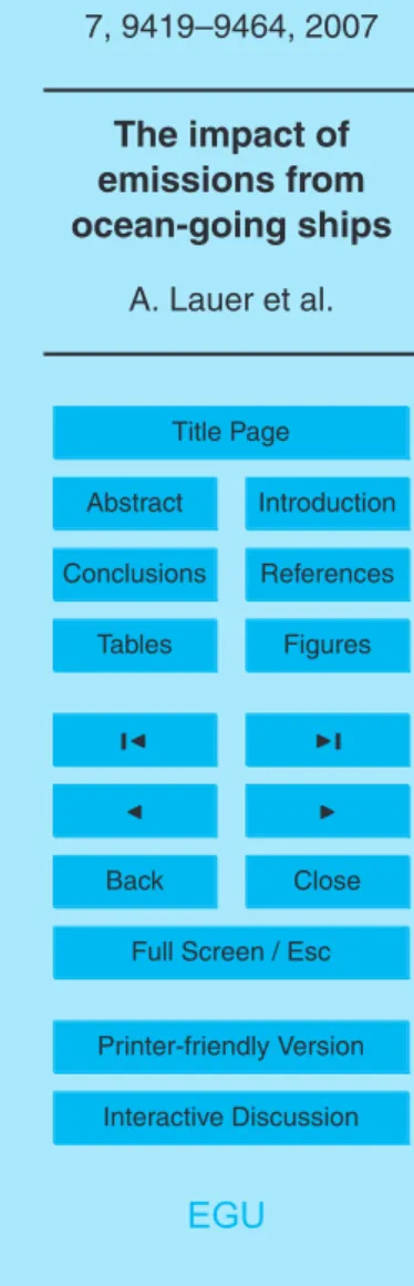
As an example, annual emissions of SO₂ from international shipping in the three different emission inventories are displayed in Fig. 1. A major amount of SO2 from

(9)

fre-ACPD

Full Screen / Esc

EGU

quented shipping routes between the eastern United States and Europe as well as between Southeast Asia and the west coast of the USA. In general emissions are low in the southern hemisphere. Differences between the emission data sets are found particularly in the Gulf of Mexico, in the Baltic, and in the northern Pacific. The Eyring et al. (2005) inventory gives the highest emissions of all three inventories in the Gulf of

5

Mexico. The Dentener et al. (2006) inventory shows higher SO₂ ship emissions in the Baltic compared to inventories A and C. Wang et al. (2007)2suggest higher emissions in the northern Pacific compared to the two other inventories.

3 Comparison to observations

The extensive intercomparison of the previous model version ECHAM4/MADE with

10

observations (Lauer et al., 2005) has been repeated with E5/M1-MADE. This inter-comparison demonstrated that the main conclusions on the model quality (Lauer et al., 2005) hold for the new model system. In particular, the main features of the observed geographical patterns, seasonal cycle and vertical distribution of the basic aerosol pa-rameters are captured. In addition to the comparison shown in Lauer et al. (2005),

15

the cloud forcing and aerosol optical thickness of the E5/M1-MADE simulation have been compared to ERBE (Earth Radiation Budget Experiment) satellite data (Bark-strom, 1984) and Aeronet (Holben et al., 1998) measurements showing reasonable good agreement in most parts of the world, including the marine areas where the largest effects of shipping are simulated. In the following subsections, we show an

20

intercomparison of model results from E5/M1-MADE using ship emission inventory A with observations focusing on marine regions. The differences between the model re-sults using inventory A and inventory B and C are rather small. It should be noted that with this evaluation we mainly evaluate the performance of the model to simulate the background atmosphere, rather than the large-scale effects (i.e. scales comparable

25

to the size of the GCM’s grid boxes) of shipping. The shipping signal cannot be easily evaluated by single-point measurements (see also Eyring et al., 2007). Processes such

(10)

ACPD

Full Screen / Esc

EGU

as long-range transport of pollutants from continental areas or natural processes are often predominant, in particular in areas close to coast. Nevertheless, this intercom-parison unveils strengths and weaknesses of the model to reproduce basic observed features relevant when assessing the impact of shipping, in particular over the oceans.

3.1 Particle number concentration

5

Clarke and Kapustin (2002) compiled vertical profiles of mean particle number concen-tration of particles greater than 3 nm from several measurement campaigns focusing on regions above the Pacific Ocean. The data include measurements performed during ACE-1, GLOBE-2, and PEM-Tropics A and B. The data have been divided into the 3 latitude bands 70◦_S–20◦_{S, 20}◦_S–20◦_{N, and 20}◦_N–70◦_{N covering longitudes between}

10

about 130◦E and 70◦W. Most of the measurements are taken over the ocean far away from the major source regions of aerosols above the continents. The variability of the particle number concentrations is given by the standard deviation. Figure 2 shows the comparison of these data to the simulated particle number concentration profiles ex-tracted for the months covered by the measurements. The model data were averaged

15

over all grid cells within the individual latitude bands.

The observed particle number concentration increases from the surface to the upper troposphere indicative of new particle formation in the upper troposphere. This is most pronounced at tropical latitudes due to strong nucleation taking place in the upper tropical troposphere. These basic features of the vertical profile of the particle number

20

concentration are reproduced by the model. In the lower troposphere of the Southern Pacific (Fig. 2, left panel), E5/M1-MADE underestimates the mean particle number concentration, which could be related to the omission of sea salt particles in the size range of the Aitken mode in the model. In the tropics (Fig. 2, middle panel) and the northern Pacific (Fig. 2, right panel), the model results are mostly within the variability

25

(11)

ACPD

Full Screen / Esc

EGU

3.2 Aerosol optical thickness (AOT)

Figure 3 shows the multi-year average seasonal cycle of the aerosol optical thickness (AOT) at 550 nm calculated by E5/M1-MADE and measured by ground based Aeronet stations (1999–2004 where data available) (Holben et al., 1997) for various small is-lands located in the Pacific (Tahiti, Coconut Island, Midway Island, Lanai), the Atlantic

5

(Azores, Capo Verde), and the Indian Ocean (Amsterdam Island, Kaashidoo, Male). These locations are considered to be basically of marine character. For comparison, also satellite data from MODIS (2000–2003) (Kaufman et al., 1997; Tanre et al., 1997), MISR (2000–2005) (Kahn et al., 1998; Martonchik et al., 1998) and a composite of MODIS, AVHRR and TOMS data (Kinne et al., 2006) are shown, as well as the

me-10

dian of several global aerosol models (Kinne et al., 2006) which provided AOT for the AeroCom Aerosol Model Intercomparison Initiative (Textor et al., 2006). The Aeronet data used are monthly means of level 2.0 AOT, version 2. The AOT data at 550 nm have been linearly interpolated from the nearest wavelengths with measurement data available.

15

For the Pacific measurement sites Coconut Island, Midway Island, and Lanai as well as for the Indian Ocean site Amsterdam Island and the Atlantic Ocean site Azores, the simulated AOT are mostly within the inter-annual variability of the Aeronet measure-ments, given by the standard deviation.

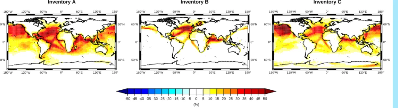
According to the geographical distribution of the ship traffic density (Fig. 3), the

mea-20

surement sites Coconut Island, Lanai, Kaashidoo, Male, Azores, and Capo Verde can be expected to be influenced by ship emissions. In contrast, ship traffic and thus emis-sions from shipping are low for all other measurement sites shown in Fig. 3 (Tahiti, Midway Island, Amsterdam Island).

E5/M1-MADE underestimates AOT compared to Aeronet observations for the sites

25

Tahiti, Kaashidoo, Male, and Capo Verde. The sites Kaashidoo and Male in the Indian Ocean are located near the Indian subcontinent. Thus, we expect the AOT measured at these sites to be influenced by continental outflow of polluted air from India, which

(12)

ACPD

Full Screen / Esc

EGU

does not seem to be reproduced by the model properly. In addition, the 2000 emis-sion data used in the model study might be too low due to the fast economic growth in these regions and thus resulting in an underestimation by the model. The measure-ment site Capo Verde in the Atlantic Ocean is located off the west coast of Africa in a latitude region characterized by easterly trade winds transporting mineral dust from

5

the deserts out onto the Atlantic Ocean. Comparisons of AOT with measurements from other regions with a high contribution of mineral dust to the total AOT indicate that E5/M1-MADE generally underestimates AOT from this aerosol component. As mineral dust is not emitted by international shipping, for the purpose of this study the detected differences between model and measurements is acceptable. However, this clearly

10

points to the need for future improvements of the representation of mineral dust in the model.

3.3 Total cloud cover

The multi-year zonal averages of total cloud cover calculated by E5/M1-MADE and obtained from ISCCP (International Satellite Cloud Climatology Project) satellite

ob-15

servations (Rossow et al., 1996) from 1983 to 2004 are shown in Fig. 4. The total cloud cover in the latitude range 60◦S to 60◦N where most ship traffic takes place is well reproduced by the model. The difference between model and satellite data is be-low 5% for most latitudes. In the polar regions, E5/M1-MADE overestimates the total cloud cover up to 20–25% near 90◦S and up to about 15% near 90◦N. The inter-annual

20

variability of the zonally averaged total cloud cover is only small, with the 1-σ standard deviation mostly below 1%. On global annual average, the simulated total cloud cover of 68% differs insignificantly from the observed total cloud cover from ISCCP of 66%. 3.4 Cloud droplet number concentration (CDNC) and effective cloud droplet radii

In a recent study, satellite observations from MODIS and AMSR-E have been used

25

(13)

ACPD

Full Screen / Esc

EGU

thickness for marine boundary layer clouds (Bennartz, 2007). The MODIS data cover the period July 2002 to December 2004. The oceanic regions we analyze here include the Pacific west of North America (155◦W–105◦W, 18◦N–39◦N), the Pacific west of South America (100◦W–60◦W, 37◦S–8◦S), the Atlantic west of North Africa (45◦W– 10◦_{W, 15}◦_N–45◦_{N), the Atlantic west of Southern Africa (20}◦_W–20◦_{E, 34}◦_S–0◦_{), and}

5

the Pacific east of Northeast Asia (110◦E–170◦E, 16◦N–35◦N).

The cloud droplet number concentrations and effective cloud droplet radii simulated by the model are calculated from the annual mean of all grid cells in the regions spec-ified above, that are defined as ocean according to the T42 land-/sea-mask of E5/M1-MADE. The altitude range of the model data covers 0.6–1.1 km. Table 2 shows the

10

model results using ship emission inventories A, B and C, as well as the model sim-ulation without ship emissions and the satellite data from MODIS and AMSR-E for average cloud droplet number concentration N and cloud droplet effective radii r. Error estimates for the cloud droplet number concentrations from the satellite data depend particularly on cloud fraction and liquid water path. For cloud fractions above 0.8 the

15

relative retrieval error in cloud droplet number concentration is smaller than 80%, for small cloud fractions (<0.1), the errors in N can be up to 260% (Bennartz, 2007).

Basically, the model and satellite data show good agreement in cloud droplet number concentration. The model data lie mostly within the observed range spanned by the standard deviation and the results obtained from the satellite data applying an

alterna-20

tive parameterization to retrieve the cloud droplet number concentration from measured effective radii and cloud optical thickness (Table 2). Bennartz (2007) concluded that marine boundary layer clouds even over the remote oceans have higher cloud droplet number concentrations in the northern hemisphere than in the southern hemisphere. This basic feature is reproduced by the model showing higher cloud droplet number

25

concentrations over the Pacific west of North America (118–127 cm−3_{) than over the}

Pacific west of South America (98–100 cm−3_{) as well as over the Atlantic west of North}

Africa (118–133 cm−3) than over the Atlantic west of Southern Africa (114–121 cm−3). Whereas the simulated cloud droplet number concentrations are in the upper range

(14)

ACPD

Full Screen / Esc

EGU

of the numbers given by the satellite data for all these oceanic regions, the simulated cloud droplet number concentrations are lower than observed over the Pacific east of Northeast Asia. This might indicate an underestimation of Asian aerosol and precursor emissions in the model, which is consistent with the findings in Sect. 3.2 for the Aeronet measurement sites Kaashidoo and Male in the Indian Ocean.

5

The effective cloud droplet radii derived from the satellite data lie between 11 µm to 13 µm. Here the model gives slightly smaller values ranging from 10 µm to 11 µm for the regions North America, North Africa, South America, and Southern Africa. For the region Northeast Asia, the average effective radii calculated by the model range from 8 µm to 9 µm, whereas the satellite data suggest 11 to 12 µm. Smaller cloud droplet

10

radii and smaller cloud droplet number concentrations indicate an underestimation of the liquid water content of low maritime clouds by the model in this region.

3.5 Cloud forcing

The cloud forcing is calculated as the difference between all-sky and clear-sky outgoing radiation at the top of the atmosphere (ToA) in the solar spectral range (shortwave cloud

15

forcing) and in the thermal spectral range (longwave cloud forcing). The cloud forcing quantifies the impact of clouds on the radiation budget (negative or positive cloud forc-ings correspond to an energy loss and a cooling effect or an energy gain and warming effect, respectively). Figure 5 shows the zonally averaged annual mean short- and longwave cloud forcing calculated by E5/M1-MADE and obtained from ERBE (Earth

20

Radiation Budget Experiment) satellite observations (Barkstrom, 1984) for the period 1985–1989. E5/M1-MADE is able to reproduce the observed shortwave cloud forcing reasonably well, i.e. the model results lie mostly within the uncertainty range of the ERBE measurements which is estimated to be about 5 W/m2. However, the model tends to overestimate the observed values (absolute values) in particular near the two

25

local maxima of the shortwave cloud forcing at about 20◦N and 20◦S. Here, deviations between model and satellite data reach up to 10 W/m2. This overestimation could be caused by the too small radii in marine stratocumuli as discussed above. It also

(15)

af-ACPD

Full Screen / Esc

EGU

fects the global annual averages. The model calculates a shortwave cloud forcing of −52.9 W/m2, the ERBE satellite data suggest a value of −47.4 W/m2.

The longwave cloud forcing calculated by E5/M1-MADE is in fairly good agreement with the ERBE observations, too. Differences between model and satellite data are below 5 W/m2 at most latitudes. The global annual averages of the longwave cloud

5

forcing are +28.0 W/m2(E5/M1-MADE) and +29.3 W/m2 (ERBE). However, the maxi-mum shown in the satellite data near the equator is not reproduced to its full extent by the model indicative of either insufficient high clouds or an underestimation of their al-titude. Maximum deviations between model and satellite data up to 12 W/m2are found in this region.

10

4 Results of the impact of shipping on aerosols and clouds

4.1 Contribution of shipping to the global aerosol

The dominant aerosol component resulting from ship emissions is sulfate, which is formed by the oxidation of SO₂by the hydroxyl radical (OH) in the gas phase or by O₃ and hydrogen peroxide (H₂O₂) in the aqueous phase of cloud droplets. Depending on

15

the ship emission inventory used, 2.3% (B,C) to 3.6% (A) of the total annual sulfate burden stems from shipping. On average, 30–40% of the simulated sulfate mass con-centration related to small particles (<1 µm) near the surface above the main shipping routes originates from shipping (Fig. 6). In contrast, contributions are smaller for black carbon emissions from shipping (0.4% in A to 1.4% in B) and particulate organic

mat-20

ter (0.1% in A to 1.1% in C), because the ship emission totals of both compounds are small compared to the contributions of fossil fuel combustion over the continents or to biomass burning. Despite high NO_xemissions from shipping, the global aerosol nitrate burden is only slightly increased by 0.1–0.2% using inventory A and B, but increased by 2.3% using inventory C. Due to the lower average SO₂ emissions in inventory C

25

(16)

ammonium-ACPD

Full Screen / Esc

EGU

nitrate forms. This results in higher aerosol nitrate concentrations. Using inventory B, aerosol nitrate is lower than using inventory C despite low SO₂ emissions. This is caused by the low NO_x emissions in inventory B compared to inventory C (Table 1). The increase in the water soluble compounds sulfate, nitrate and associated ammo-nium causes an increase in the global burden of aerosol liquid water contained in the

5

optically most active particles in the sub-micrometer size-range. This liquid water in-crease amounts to 4.3% (A), 2.2% (B), and 3.5% (C). Table 3 summarizes the total burdens and the relative contribution of shipping for the aerosol compounds consid-ered in E5/M1-MADE for all three ship emission inventories.

The model calculates a ship induced increase in the particle number concentration

10

of the Aitken mode particles (typically smaller than 0.1 µm) of about 40% near the sur-face above the main shipping region in the Atlantic Ocean. Furthermore, the average geometric mean diameter of these particles decreases from 0.05 µm to 0.04 µm as the freshly emitted particles from shipping are smaller than the aged Aitken particles typically found above the oceans far away from any continental source. Subsequent

15

processes such as condensation of sulfuric acid vapor enable some particles to grow into the next larger size-range, the accumulation mode (0.1 to 1 µm), increasing the number concentration in this mode. Accumulation mode particles act as efficient con-densation nuclei for cloud formation. The model results indicate that the accumulation mode particle number concentration in the lowermost boundary layer above the main

20

shipping routes in the Atlantic Ocean is increased by about 15%. In contrast to the Aitken mode, the average modal mean diameter of the simulated accumulation mode is not affected by ship emissions and remains almost constant.

The changes in particle number concentration, particle composition and size-distribution result in an increase in aerosol optical thickness above the oceans of

typ-25

ically 2–3% (Fig. 7, upper row). Depending on the inventory used, different amounts of emissions are assigned to specific regions. This leads to differences in the results. Individual regions such as the Gulf of Mexico show increases up to 8–10% (A), the Northeastern Pacific up to 6% (C), and the highly frequented shipping route through

(17)

ACPD

Full Screen / Esc

EGU

the Red Sea (Suez Canal) to the tip of India in the Indian Ocean up to 10–14% (A, B, C). This effect is mainly related to enhanced scattering of solar radiation by sulfate, nitrate, ammonium, and associated aerosol liquid water. The calculated changes in the global annual average clear-sky top of the atmosphere (ToA) solar radiative flux are −0.038 W/m2 (A), −0.012 W/m2 (B), and −0.030 W/m2 (C). Local changes up to

5

−0.25 W/m2 are simulated for the Gulf of Mexico (A), the Northeastern Pacific (C), or the highly frequented regions of the Indian Ocean (A, B, C). These regions can also be identified in the zonal averages (Fig. 7, lower row). The contribution to changes in the clear-sky ToA thermal flux due to shipping is negligible and not statistically significant compared to its statistical fluctuations.

10

The changes in the simulated clear-sky fluxes do not represent the global average direct aerosol effect because clouds can have a strong impact on the radiation field. The simulations carried out in this study include both, the direct and the indirect aerosol effect. Thus, the all-sky direct aerosol effect cannot be separated from changes in the radiation fluxes due to the indirect aerosol effect. To estimate the changes in the

all-15

sky radiation fluxes due to the direct aerosol effect, an additional assumption has to be made. Here we assume that the direct aerosol effect is relevant in the cloud free areas of each grid cell only and negligible in the cloudy areas. According to our simulations, the signal from shipping on aerosols decays rapidly with altitude. Consequently, a major fraction of the aerosols from shipping is below the clouds (or inside the clouds

20

in case of very low clouds) damping the impact of these aerosol particles on the ToA radiation fluxes in cloudy areas. We then can scale the change in the clear-sky fluxes in each grid cell by (1 – total cloud cover) to estimate the all-sky direct aerosol effect:

∆RFsolar(all-sky) = (1 − total cloud cover) · ∆RFsolar(clear-sky) (1)

Using this simple approximation, we estimate the direct aerosol effect from shipping to

25

amount −0.014 W/m2(A), −0.010 W/m2(B), and −0.009 W/m2 (C). However, it should be kept in mind that this approximation gives an estimate for the direct aerosol effect only, because the presence of clouds can modify the radiation field dramatically and thus change the radiative forcing of aerosols in the cloudy fraction of the grid box.

(18)

ACPD

Full Screen / Esc

EGU

Consequently, the true all-sky direct aerosol RF can only be approximated by the cloud cover area-weighted clear-sky RF given by Eq. (1).

4.2 Modification of cloud microphysical properties

The second important effect of the aerosol changes due to ship emissions is a modifi-cation of cloud microphysical properties. The model simulations reveal that this effect

5

is mainly confined to the lower troposphere from the surface up to about 1.5 km. This implies that regions with a frequent high amount of low clouds above the oceans are most susceptible for modifications due to ship emissions. Such regions are coincid-ing with dense ship traffic over the Pacific Ocean west of North America, the Atlantic Ocean west of Southern Africa and the Northeastern Atlantic Ocean (Fig. 8). These

10

regions are consistent with the locations showing the maximum response in the indirect aerosol effect due to shipping calculated by E5/M1-MADE.

Whereas the vertically integrated cloud liquid water content is only slightly (1–2%) af-fected by ship emissions and the ice crystal number concentration shows no significant change, simulated cloud droplet number concentrations are significantly increased.

15

Maximum changes of the cloud droplet number are computed above the main shipping routes in the Atlantic and Pacific Ocean at an altitude of about 500 m. These changes in cloud droplet number concentration amount to 30–50 cm−3_{(20–30%) in the Atlantic}

(A, B, C) and about 20–40 cm−3 (15–30%, A, C) and 5–15 cm−3(5–10%, B) in the Pa-cific. The corresponding changes in cloud liquid water content at this altitude calculated

20

by the model show an increase in the order of a few percent, but are statistically not significant. The increase in cloud droplet number causes a decrease in the effective radius of the cloud droplets. In the Atlantic Ocean, for instance, the average decrease in the cloud droplet effective radius is 0.42 µm (A), 0.17 µm (B), and 0.25 µm (C) at an altitude of 0.4 km. This effect results in an enhanced reflectivity of these low

ma-25

rine clouds. Figure 9 depicts the annual mean changes in zonal average cloud droplet number concentrations, cloud droplet effective radii, and cloud optical thickness in the spectral range 0.28–0.69 µm due to shipping for the three emission inventories. The

(19)

ACPD

Full Screen / Esc

EGU

increase in cloud droplet number concentration and the decrease in cloud droplet ef-fective radii result in an increase in cloud optical thickness of typically 0.1 to 0.3 on zonal annual average. Whereas the changes in cloud optical thickness are limited to the latitude range 0◦ to 70◦N for inventory B, statistically significant changes are cal-culated between 60◦_{S to 60}◦_{N for inventory A with maximum changes in cloud optical}

5

thickness up to about 0.5 in the latitude range around 20◦_{N to 30}◦_N.

The simulated shipping-changes in the annual mean total cloud cover, the geograph-ical precipitation patterns or the total precipitation are statistgeograph-ically not significant com-pared to the inter-annual variability.

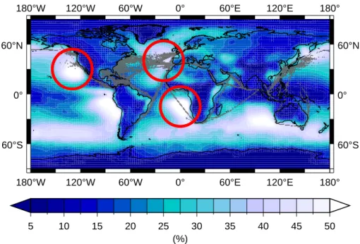
The increased reflectivity of the low marine clouds results in an increased

short-10

wave cloud forcing, calculated as the difference between the whole sky value and the clear-sky value of the net shortwave radiation at the ToA. The shortwave cloud forc-ing quantifies the impact of clouds on the Earth’s radiation budget in the solar spectral range. Figure 10 shows the geographical distribution of the 6-year annual average changes in ToA shortwave cloud forcing and the corresponding zonal means for the

15

three ship emission inventories A, B, and C. Statistically significant changes in the shortwave cloud forcing are found in particular above the Pacific off the west coast of North America (A, C), the Northeastern Atlantic (A, B, C) and above the Atlantic off the west coast of Southern Africa (A, C). Local changes in the Pacific and Atlantic can reach −3 to −5 W/m2 (A, C) and −2 to −3 W/m2 (B). In contrast, changes above the

20

Indian Ocean are smaller despite the high ship traffic density. This is due to the low cloud amount susceptible to ship emissions being rather low in this region (Fig. 8). Sim-ulated changes in the longwave cloud forcing (thermal spectral range) are small and statistically not significant because of the comparably low temperature differences be-tween the sea surface temperature and the cloud top height of the low marine clouds.

25

Changes in the zonally averaged annual mean cloud forcing for the solar spectrum due to ship emissions are mostly confined to the latitude range 40◦_{S to 50}◦_{N (A), 10}◦_{N to}

50◦N (B), and 30◦S to 50◦N (C). Table 4 summarizes the annual average changes in shortwave cloud forcing for all three emission inventories and different regions. The

(20)

ACPD

Full Screen / Esc

EGU

global annual mean changes in the shortwave cloud forcing amount to −0.6 W/m2(A), −0.19 W/m2(B), and −0.44 W/m2(C).

A comparison of the results with E5/M1-MADE simulations using pre-industrial emis-sions for trace gases (van Aardenne et al., 2001) and particles (Dentener et al., 2006) results in a total anthropogenic indirect aerosol effect (including ships) of −1.1 W/m2

5

(B) to −1.5 W/m2 (A). These values are within the range of previous model estimates (−0.9 to −2.9 W/m2) (Lohmann and Feichter, 2005) of the total anthropogenic indirect effect. According to the results of our model studies, shipping contributes to about 17% (B) to 39% (A) to the total anthropogenic indirect effect. This contribution is larger than the contribution of shipping to aerosol emissions, because of larger albedo changes by

10

clouds over dark oceans than over land. In addition, this effect is comparatively large since ship emissions are released in regions with frequent occurrence of low clouds, which are highly susceptible to the enhanced aerosol number concentration in an oth-erwise clean marine environment. For both reasons, the susceptibility of the radiation budget to ship emissions is much higher than for continental anthropogenic aerosol

15

sources of the same source strength. Simple scaling of the total anthropogenic indirect aerosol effect to the contribution of an individual source to the total atmospheric burden is therefore questionable for shipping.

4.3 Radiative forcing due to international shipping

The indirect aerosol effect of shipping on climate discussed in Sect. 4.2 results in a

20

negative radiative forcing (RF) which is, in absolute numbers, much higher than the negative RF caused by the scattering and absorption of solar radiation by aerosol par-ticles (direct aerosol effect) or the positive RF due to greenhouse gases, mainly carbon dioxide and ozone. NO_x and other ozone precursor emissions from shipping not only perturb the atmosphere by the formation of O₃, but also lead to enhanced levels of OH,

25

increasing removal rates of CH₄, thus generating a negative radiative forcing. These previously estimated forcings are all in the range of ±15 to 50 mW/m2 (Endresen et

(21)

ACPD

Full Screen / Esc

EGU

al., 2003; Eyring et al., 2007). RF due to direct CH₄from shipping (0.52 Tg CH₄ from fuel and tanker loading; Eyring et al., 2005a) has not been estimated so far. How-ever, because of the small contribution (<0.2%) to total anthropogenic CH₄ emissions (Olivier et al., 2005), the resulting forcings are expected to be negligible compared to the other components. Figure 11 shows the RF due to shipping from CO₂, O₃,

5

CH₄, and the direct effect of SO4 particles from Endresen et al. (2003) and Eyring et

al. (2007) as well as the radiative forcing due to ship tracks (Schreier et al., 20071) in comparison to the estimated direct aerosol effect (Sect. 4.1) and indirect aerosol effect (Sect. 4.2) obtained in this study for the three ship emission inventories A, B, and C. Schreier et al. (2006) showed that ship tracks can change the radiation budget on a

10

local scale, but are short lived and cover a very small fraction of the globe so that their radiative effect on the global scale is negligible (−0.4 to −0.6 mW/m2±40%; Schreier et al., 20071). The contribution of water vapor emissions from shipping is also negligible. Also shown is a previous estimate by Capaldo et al. (1999), who used a global model without detailed aerosol microphysics and aerosol-cloud interaction and assessed the

15

first indirect effect of SO4 plus organic material particles (−0.11 W/m2). In contrast to

Capaldo et al. (1999), Endresen et al. (2003) and Eyring et al. (2007), the model study presented here considers not only sulfate, but changes in the radiation budget due to the sum of all relevant aerosol components (SO₄, NO₃, NH₄, BC, POM, and aerosol liquid water).

20

The model results discussed in Sects. 4.1 and 4.2 and shown in Fig. 11 also in-dicate that the geographical distribution of emissions over the globe plays a key role determining the global impact of shipping. The large differences in the model results obtained with three different ship emission inventories (Eyring et al., 2005; Dentener et al., 2006; Wang et al., 20072) imply a high uncertainty, but on the other hand the

25

main conclusions of this study hold for all three inventories. For all inventories used, the present-day net RF from ocean-going ships is strongly negative, in contrast to, for instance, estimates of RF from aircraft (Sausen et al., 2005). In addition, the direct aerosol effect due to scattering and absorption of solar light by particles from shipping

(22)

ACPD

Full Screen / Esc

EGU

is only of minor importance compared to the indirect aerosol effect. Additional sen-sitivity simulations with sulfur free fuel with E5/M1-MADE revealed that about 75% of the direct and indirect aerosol effect from shipping is related to the fuel sulfur content, which is currently about 2.4% (EPA, 2002). Thus, a simple upscaling of the results from Capaldo et al. (1999) to the total indirect effect considering all relevant aerosol

com-5

pounds from shipping results in about −0.15 W/m2. This value is comparable to the indirect aerosol effect calculated in this study using inventory B (−0.19 W/m2). Inven-tory B has similar emission totals for SO₂(7.8 Tg yr−1_{) as the ship emission inventory}

used by Capaldo et al. (1999) totaling 8.4 Tg yr−1_.

5 Summary and conclusions

10

In this study we used the general circulation model ECHAM5/MESSy1 coupled to the aerosol module MADE (E5/M1-MADE) to study the impact of shipping on aerosols, clouds and the Earth’s radiation budget. The aerosols calculated by E5/M1-MADE are used to drive the radiation and cloud scheme of the GCM allowing to assess both, the direct and indirect aerosol effect of emissions from shipping. The evaluation of the

15

model showed that the main features of the observed geographical patterns, seasonal cycle and vertical distribution of the basic aerosol parameters are captured. However, the comparison also unveiled still existing weaknesses of the model such as represent-ing the optical properties of mineral dust or capturrepresent-ing Asian emissions of particulate matter and aerosol precursors. For the purpose of this study, these model deficiencies

20

are acceptable when assessing the impact of shipping on aerosols and clouds by cal-culating differences between model simulations with and without taking into account ship emissions.

To assess uncertainties in estimates of present-day emission totals and spatial ship traffic proxies, we used three different present-day (year 2000 conditions) ship emission

25

inventories, Eyring et al. (2005) (inventory “A”), Dentener et al. (2006) (inventory “B”), and Wang et al. (2007)2(inventory “C”) and one simulation without ship emissions. The

(23)

ACPD

Full Screen / Esc

EGU

impact of emissions from international shipping on the chemical composition, particle number concentration, and size distribution of atmospheric aerosol has been assessed by analyzing the differences between model simulations with and without shipping. In order to obtain significant differences with a reasonable number of model years, model dynamics have been nudged using operational analysis data from the European

Cen-5

tre for Medium-Range Weather Forecasts (ECMWF) from 1999 to 2004. The changes in aerosol properties affect the optical properties such as aerosol optical thickness of the particles (direct aerosol effect) as well as their ability to act as cloud condensa-tion nuclei (indirect aerosol effect). Both mechanisms that impact the Earth’s radiacondensa-tion budget are taken into account in the E5/M1-MADE simulations.

10

The model results reveal that the most important aerosol component from shipping is SO₄, formed by the oxidation of SO₂emitted by ships, contributing 2.3% to 3.6% to the total atmospheric sulfate burden in the simulations with different emission scenar-ios performed here. The contribution of BC and POM from shipping is only 0.4–1.4% and 0.1–1.1%, respectively. Aerosol nitrate from shipping shows the highest sensitivity

15

to the emission inventory and contributes between 0.1% and 2.3% to the total aerosol nitrate burden. The signal from shipping decays rapidly with altitude, and is mostly lim-ited to the lowermost 1.5 km in the troposphere. The model results show an increase in the Aitken mode particle number concentration of about 40% in the near surface layer above the main shipping routes in the Atlantic Ocean and a decrease in the modal

20

mean diameter of the Aitken mode from 0.05 µm to 0.04 µm in this region. Due to subsequent growth processes such as condensation of sulfuric acid vapor and coagu-lation, some particles grow into the next larger size-range of the accumulation mode, which can act as additional cloud condensation nuclei. These changes in chemical composition, particle number concentration, and size-distribution cause an increase in

25

aerosol optical thickness above the oceans, which is related particularly to enhanced scattering of incoming solar radiation by sulfate, nitrate, ammonium, and associated aerosol liquid water. Local changes up to −0.25 W/m2 are simulated in individual re-gions such as the Gulf of Mexico, the Northeastern Pacific or the highly frequented

(24)

ACPD

Full Screen / Esc

EGU

regions in the Indian Ocean, depending on the emission inventory used. The calcu-lated global annual average changes in the clear-sky top of the atmosphere radiative fluxes in the solar spectrum range from −0.012 W/m2 to −0.038 W/m2, the estimated (Eq. 1) corresponding direct aerosol effects range from −0.009 W/m2to −0.014 W/m2. The by far most important impact of ship emissions on the radiation budget is related

5

to changes in the microphysical properties of low marine clouds. The simulations re-vealed that emissions from international shipping impact the Earth’s radiation budget significantly and more than previously estimated from model studies without detailed aerosol microphysics and aerosol-cloud interaction using older ship emission invento-ries with lower emission totals (−0.11 W/m2) (Capaldo et al., 1999). The changes in

10

the radiation budget caused by modified cloud properties from the three different ship emission inventories range from −0.19 W/m2to −0.6 W/m2. The regions affected are in particular the Northeastern Pacific off the west coast of North America, the Northeast-ern Atlantic, and the Atlantic off the west coast of SouthNortheast-ern Africa. These regions are characterized by frequent occurrence of low marine clouds and coinciding high ship

15

traffic density. The model results show that the impact of shipping is mostly confined to liquid water clouds. Ice clouds are hardly influenced. This is related to the fact, that liquid water clouds are the dominant cloud type in the regions and in the altitude range (<1.5 km) predominantly affected by shipping. The additional cloud condensa-tion nuclei from shipping increase the cloud droplet number concentracondensa-tion of the marine

20

clouds, whereas the simulated liquid water content is only slightly changed. This re-sults in a decrease of the cloud droplet effective radii increasing the reflectivity of the marine clouds and thus enhancing the shortwave cloud forcing. Sensitivity studies us-ing pre-industrial emissions suggest that shippus-ing contributes between 17% and 39% to the total anthropogenic indirect aerosol effect. This large contribution is related to the

25

larger albedo changes by clouds over dark oceans than over land and to the fact that ship emissions are released in regions with frequent occurrence of low clouds, which are highly susceptible to the enhanced aerosol number concentration in an otherwise clean marine environment. This results in a much higher response for shipping than

(25)

ACPD

Full Screen / Esc

EGU

for continental anthropogenic aerosol sources of the same source strength.

The net RF from shipping, calculated from previous estimates of the RF from CO₂, O₃, and CH₄ from shipping as well as from the direct and indirect aerosol ef-fect estimated here, is negative for all three emissions inventories ranging between −0.16 W/m2and −0.58 W/m2. Further sensitivity studies with sulfur free fuel show that

5

about 75% of both, the direct and indirect aerosol effect from shipping, are related to the fuel sulfur content. Carbon dioxide’s atmospheric lifetime (>100 years) is much longer than global atmospheric mixing timescales, so ship CO₂ emissions generate a radiative forcing in just the same way as any other CO₂ source. In the future, the positive RF from shipping CO₂ is expected to increase, because of the expected CO₂

10

emission growth from the ocean-going fleet (Eyring et al., 2005b). All other RF con-tributions strongly depend on the technology applied. Future reductions in SO₂ from ships are to be expected because of air quality issues in the vicinity of major harbors and because of the acidification of the oceans due to sulfate and sulfur emissions. The first sulfur emission control area (SECA, with only 1.5% sulfur content) in the Baltic

15

Sea was established in May 2006. The next SECA is planned for parts of the English Channel and the North Sea and will enter into force in 2007. Furthermore, the Euro-pean Union has disbanded the Directive 2005/33/EC, to limit the sulfur content to 0.1% in marine fuels for harbor regions in 2010. If the sulfur content of the fuel is reduced, the positive contributions to the overall RF from CO₂will remain, whereas the negative

20

RF due to the effect on aerosols and clouds will strongly decrease. However, because of air quality issues and acidification as a consequence of ship sulfur emissions, en-hanced shipping with sulfur-rich fuel should not be considered as a geo-engineering strategy to decelerate global warming.

This study also showed that the geographical distribution of ship emissions over the

25

globe plays a key role determining the global impact of shipping. The large differences in the model results obtained with three different ship emission inventories (Eyring et al., 2005; Dentener et al., 2006; Wang et al., 20072) imply a high uncertainty. Never-theless, the main conclusions of this study hold for all three inventories. We therefore

(26)

ACPD

Full Screen / Esc

EGU

conclude that the impact of ship exhaust on atmosphere and climate has received too little attention so far and should be subject to further investigations. In particular, it remains a challenge to reduce uncertainties in present-day emission inventories, both in the emission total estimates as well as in the spatial ship traffic proxies. In addi-tion, modeling of the indirect aerosol effect introduces still many uncertainties. Critical

5

model parameters and processes are in particular the aerosol size-distribution and particle number concentration (Penner et al., 2006) as well as the parameterization of aerosol activation (Lohmann and Feichter, 2005).

Acknowledgements. This work was supported by the German Helmholtz-Gemeinschaft

Deutscher Forschungszentren (HGF) and the Deutsches Zentrum f ¨ur Luft- und Raumfahrt 10

(DLR) within the Young Investigators Group SeaKLIM and the project Particles and Cirrus Clouds (PAZI-2). We wish to thank the whole MESSy team of the Max Planck Institute for Chemistry in Mainz, Germany for their support and help and the Max Planck Institute for Mete-orology in Hamburg, Germany for the development and provision of ECHAM5. We also kindly acknowledge the provision of MADE by the University of Cologne, Germany (RIU/EURAD-15

project) and thank U. Schumann and R. Sausen for very helpful discussions. All model simu-lations were performed on the High Performance Computing Facility (HPCF) at the European Centre for Medium-Range Weather Forecasts (ECMWF).

References

Abdul-Razzak, H. and Ghan, S. J.: A parameterization of aerosol activation, 2. Multiple aerosol 20

types, J. Geophys. Res., 105(D5), 6837–6844, 2000.

Ackermann, I. J., Hass, H., Memmesheimer, M., Ziegenbein, C., and Ebel, A.: Modal Aerosol Dynamics for Europe: Development and first applications, Atmos. Environ., 32, 2981–2999, 1998.

Barkstrom, B. R.: The Earth Radiation Budget Experiment (ERBE), Bull. Amer. Meteor. Soc., 25

65, 1170–1185, 1984.

Bennartz, R.: Global assessment of marine boundary layer cloud droplet number concentration from satellite, J. Geophys. Res., 112, D02201, doi:10.1029/2006JD007547, 2007.

(27)

ACPD

Full Screen / Esc

EGU

Capaldo, K., Corbett, J. J., Kasibhatla, P., Fischbeck, P. S., and Pandis, S. N.: Effects of ship emissions on sulfur cycling and radiative climate forcing over the ocean, Nature, 400, 743– 746, 1999.

Clarke, A. D. and Kapustin, V. N.: A Pacific Aerosol Survey. Part I: A Decade of Data on Particle Production, Transport, Evolution, and Mixing in the Troposphere, J. Atmos. Sci., 59, 363–382, 5

2002.

Corbett, J. J. and Koehler, H. W.: Updated emissions from ocean shipping, J. Geophys. Res., 108(D20), 4650, doi:10.1029/2003JD003751, 2003.

Dentener, F., Kinne, S., Bond, T., Boucher, O., Cofala, J., Generoso, S., Ginoux, P., Gong, S., Hoelzemann, J. J., Ito, A., Marelli, L., Penner, J. E., Putaud, J.-P., Textor, C., Schulz, M., 10

van der Werf, G. R., and Wilson, J.: Emissions of primary aerosol and precursor gases in the years 2000 and 1750, prescribed data-sets for AeroCom, Atmos. Chem. Phys., 6, 4321– 4344, 2006,

http://www.atmos-chem-phys.net/6/4321/2006/.

Durkee, P. A., Chartier, R. E., Brown, A., Trehubenko, E. J., Rogerson, S. D., Skupniewicz, C., 15

Nielsen, K. E., Platnick, S., and King, M. D.: Composite Ship-Track Characteristics, J. Atmos. Sci., 57, 2542–2553, 2000.

Endresen, Ø., Sørg ˚ard, E., Sundet, J. K., Dalsøren, S. B., Isaksen, I. S. A., Berglen, T. F., and Gravir, G.: Emission from international sea transportation and environmental impact, J. Geophys. Res., 108(D17), 4560, doi:10.1029/2002JD002898, 2003.

20

EPA (Environmental Protection Agency, USA.): SPECIATE 3.2, profiles of total organic com-pounds and particulate matter, http://www.epa.gov/ttn/chief/software/speciate/index.html, 2002.

Eyring, V., K ¨ohler, H. W., van Aardenne, J., and Lauer, A.: Emissions from international ship-ping, Part 1: The last 50 years, J. Geophys. Res., 110(D17305), doi:10.1029/2004JD005619, 25

2005a.

Eyring, V., K ¨ohler, H. W., Lauer, A., and Lemper, B.: Emissions From International Shipping: 2. Impact of Future Technologies on Scenarios Until 2050, J. Geophys. Res., 110(D17306), doi:10.1029/2004JD005620, 2005b.

Eyring, V., Stevenson, D. S., Lauer, A., Dentener, F. J., Butler, T., Collins, W. J., Ellingsen, K., 30

Gauss, M., Hauglustaine, D. A., Isaksen, I. S. A., Lawrence, M. G., Richter, A., Rodriguez, J. M., Sanderson, M., Strahan, S. E., Sudo, K., Szopa, S., van Noije, T. P. C., and Wild, O.: Multi-model simulations of the impact of international shipping on atmospheric chemistry

(28)

ACPD

Full Screen / Esc

EGU

and climate in 2000 and 2030, Atmos. Chem. Phys., 7, 757–780, 2007,

Hobbs, P. V., Garrett, T. J., Ferek, R. J., Strader, S. R., Hegg, D. A., Frick, G. M., Hoppel, W. A., Gasparovic, R. F., Russel, L. M., Johnson, D. W., O’Dowd, C., Durkee, P. A., Nielsen, K. E., and Innis, G.: Emissions from ships with their respect to clouds, J. Atmos. Sci., 57, 5

2570–2590, 2000.

Holben, B., Eck, T., Slutsker, I., Tanre, D., Buis, J., Vermote, E., Reagan, J., Kaufman, Y., Naka-jima, T., Lavevau, F., Jankowiak, I., and Smirnov, A.: AERONET – A federated instrument network and data archive for aerosol characterization, Rem. Sens. Environ., 66, 1–16, 1998. J ¨ockel, P., Sander, R., Kerkweg, A., Tost, H., and Lelieveld, J.: Technical Note: The Modular 10

Earth Submodel System (MESSy) – a new approach towards Earth System Modeling, At-mos. Chem. Phys., 5, 433–444, 2005,

J ¨ockel, P., Tost, H., Pozzer, A., Br ¨uhl, C., Buchholz, J., Ganzeveld, L., Hoor, P., Kerk-weg, A., Lawrence, M. G., Sander, R., Steil, B., Stiller, G., Tanarhte, M., Taraborrelli, D., 15

van Aardenne, J., and Lelieveld, J.: The atmospheric chemistry general circulation model ECHAM5/MESSy1: consistent simulation of ozone from the surface to the mesosphere, At-mos. Chem. Phys., 6, 5067–5104, 2006,

Kahn, R., Banerjee, P., McDonald, D., and Diner, D. J.: Sensitivity of multi-angle imaging to 20

aerosol optical depth and to pure particle size distribution and composition over ocean, J. Geophys. Res., 103, 32 195–32 213, 1998.

Kaufman, Y., Tanre, D., Remer, L., Vermote, E., Chu, D., and Holben, B.: Operational remote sensing of tropospheric aerosol over the land from EOS-MODIS, J. Geophys. Res., 102, 17 051–17 061, 1997.

25

Kerkweg, A., Buchholz, J., Ganzeveld, L., Pozzer, A., Tost, H., and J ¨ockel, P.: Technical Note: An implementation of the dry removal processes DRY DEPosition and SEDImentation in the Modular Earth Submodel System (MESSy), Atmos. Chem. Phys., 6, 4617–4632, 2006a. Kerkweg, A., Sander, R., Tost, H., and J ¨ockel, P.: Technical note: Implementation of prescribed

(OFFLEM), calculated (ONLEM), and pseudo-emissions (TNUDGE) of chemical species in 30

the Modular Earth Submodel System (MESSy), Atmos. Chem. Phys., 6, 3603–3609, 2006b. Kinne, S., Schulz, M., Textor, C., Guibert, S., Balkanski, Y., Bauer, S. E., Berntsen, T., Berglen,