HAL Id: hal-03105806
https://hal.archives-ouvertes.fr/hal-03105806
Submitted on 11 Jan 2021
HAL is a multi-disciplinary open access
archive for the deposit and dissemination of
sci-entific research documents, whether they are
pub-lished or not. The documents may come from
teaching and research institutions in France or
abroad, or from public or private research centers.
L’archive ouverte pluridisciplinaire HAL, est
destinée au dépôt et à la diffusion de documents
scientifiques de niveau recherche, publiés ou non,
émanant des établissements d’enseignement et de
recherche français ou étrangers, des laboratoires
publics ou privés.
Guodong Gai, Olivier Thomine, Abdellah Hadjadj, Sergey Kudriakov
To cite this version:
Guodong Gai, Olivier Thomine, Abdellah Hadjadj, Sergey Kudriakov. Modeling of particle cloud
dispersion in compressible gas flows with shock waves. Physics of Fluids, American Institute of
Physics, 2020, 32 (2), pp.023301. �10.1063/1.5135774�. �hal-03105806�
compressible gas flows with shock waves
Cite as: Phys. Fluids 32, 023301 (2020); https://doi.org/10.1063/1.5135774Submitted: 08 November 2019 . Accepted: 14 January 2020 . Published Online: 03 February 2020 Guodong Gai , Olivier Thomine, Abdellah Hadjadj, and Sergey Kudriakov
ARTICLES YOU MAY BE INTERESTED IN
Numerical study on shock-accelerated gas rings
Physics of Fluids
32, 026102 (2020);
https://doi.org/10.1063/1.5135762
Stability of a vertical Couette flow in the presence of settling particles
Physics of Fluids
32, 024104 (2020);
https://doi.org/10.1063/1.5140422
Linear and weakly nonlinear stability analysis on a rotating anisotropic ferrofluid layer
Modeling of particle cloud dispersion
in compressible gas flows with shock waves
Cite as: Phys. Fluids 32, 023301 (2020);doi: 10.1063/1.5135774
Submitted: 8 November 2019 • Accepted: 14 January 2020 • Published Online: 3 February 2020
Guodong Gai,1,2,a) Olivier Thomine,1 Abdellah Hadjadj,2 and Sergey Kudriakov1 AFFILIATIONS
1DEN-DM2S-STMF, Commissariat à l’Énergie Atomique et aux Énergies Alternatives, Université Paris-Saclay,
91191 Gif-sur-Yvette, France
2University of Normandy, INSA, CORIA UMR - 6614 CNRS, 76000 Rouen, France
a)Author to whom correspondence should be addressed:guodong.gai@cea.fr
ABSTRACT
The effect of shock waves on the dispersion characteristics of a particle cloud is investigated both numerically and analytically. A one-dimensional analytical model is developed for the estimation of the cloud topology in the wake of a shock wave, as a function of time, space, and characteristic response time τpof the cloud based on the one-way formalism. The model is compared with the results obtained
with numerical simulations over a wide range of incident Mach numbersMsand particle volume fraction τv,0. An extension of the one-way
formalism to the two-way is proposed by taking into account the post-shock gas deceleration due to the presence of particles. A significant increase in the cloud density is noticed. The effects of different parameters affecting the shock–spray interaction are elucidated and discussed. The two-way formalism is seen to better describe the effects of the particles on the propagation of the shock wave.
Published under license by AIP Publishing.https://doi.org/10.1063/1.5135774., s
I. INTRODUCTION
The interaction between shock waves and particles has been an active research field for decades.1–5Many theoretical and experi-mental studies are conducted in order to understand the interaction mechanisms of shock waves with droplets or solid particles,6–10since it is present and of major importance in various industrial applica-tions. For instance, the compression waves can coalesce and generate shock waves in internal engines.11The shocked fuel spray has differ-ent dispersion topologies, thus changing the combustion properties. Other applications concern explosion in the confinement building, where the shock waves can be initiated accidentally. In order to mit-igate their effects, an aqueous foam12–15or a water spray system16 can be used. In this case, the shock–spray interaction can change dramatically the dispersion of droplets, leading to the change in the mitigation capacity of the spray system.17–19On the contrary, the particle cloud can also affect the propagation of the shock wave.20
Basically, as a result of the high velocity of the shocked gas, the shock–droplet interaction can generate complex coupled phenom-ena such as droplet deformation, atomization, collision, coalescence, and evaporation.11,21,22Moreover, the polydispersion of the droplets
adds further difficulties to the investigations. To simplify the prob-lem, various studies focus on the interaction between a shock wave and a single or an array of particles,23–25where the effects of par-ticles on gas flow are weak. Dense particle or particle curtains are also investigated,3,26in which the collision between the particles is important.
Given the complexity of the droplet behavior during the inter-action, rigid particles of uniform diameters are commonly used to simplify the shock–particle interaction. Even though the qual-itative phenomena are well known,1,3 the interaction mechanisms between shock and particles are yet to be elucidated quantitatively in both well-conducted experiments and in numerical simulations and modelings.27 Particularly, the particle clouds of the volume fraction O(10−4–10−3) are of great interest in nuclear industrial applications.
The integral properties of the particle cloud movements such as volume fraction distribution and velocity distribution are also important for the large-scale simulations.28 However, to the best knowledge of the authors, the existing particle-resolved models for simulations of large-scale geometries such as nuclear confinement building are scarce, as a result of high computational expenses, espe-cially for high Reynolds number flows. Thus, simple reduced-order
modeling approaches and empirical correlations are considered to be the alternative solutions.
In this study, a new analytical model is developed to quantify the shocked gaseous flow impact on the dispersed phase using a one-way formalism. An extended two-one-way theoretical model is proposed, which takes into consideration the deceleration effect of the particles on the gas phase. The objectives of this study are threefold: (i) pro-vide a simplified analytical formulation of particle cloud dispersion after the interaction with a shock wave, (ii) elucidate the importance of the two-way formalism on the description of the shock–cloud interaction, and (iii) identify the main parameters and their effects on the shock–cloud interaction. The theoretical model is validated with high-resolved numerical simulations.
This paper is organized as follows: SectionIIdiscusses the char-acteristics of the particle cloud. SectionIIIpresents an analytical formulation of particle dispersion with a shock wave. Section IV
discusses the assessment of the analytical model, and the compar-isons between the analytical results and the numerical simulations are presented in Sec.V. Finally, the main conclusions together with recommendations for future work are given in Sec.VI.
II. CHARACTERISTICS OF THE CLOUD PARTICLES In this study, assumptions are made so that the gas is consid-ered as inviscid and follows the perfect-gas law, the particles are supposed to be rigid and spherical, with small volume fractions, the collisions between them are neglected,29only viscous drag forces act on the particles, and the heat transfer between gas and particles is neglected.
Initially at rest, the particles are assumed to be uniformly dis-tributed throughout the computational domain. After the passage of the shock, the particles are accelerated by the gas flow. In order to determine the evolution of the particles, we compute the force applied by the flow of velocity u(x,t) on a spherical particle of coor-dinate x, with a velocity V(t) and a diameter dp. The general equation
of motion reads
mpdV(t)
dt = ∑F, (1)
wheremp=πρpd3p/6 is the particle mass and ρpis the particle density.
Here, we neglect the gravity, the Magnus’ force, and the Basset force as a result of the high ratio between the densities of the liquid and gas phases. The viscous drag force gives
F =π 8ρpd
2
pCD∣u(x,t) − V(t)∣(u(x, t) − V(t)), (2) whereCDis the drag coefficient of the particles defined as
CD= 24
Rep, with
Rep=
ρg∣u(x,t) − V(t)∣dp
μg , (3)
where Rep is the particular Reynolds number related to the flow
around the particle and μgis the dynamic viscosity of the gas. The
diameters of the particles considered in this study vary from 10 nm to 50 μm. Due to the small size of particles, the drag coefficient is given by the Stokes coefficient for laminar flow. The equation of motion for each particle can be obtained as
dV(t) dt = 1 τp (u(x,t) − V(t)), with τp= ρpd2p 18μg . (4)
In the case of a two-way interaction, and in order to estimate the effect of the particles on the gas, the momentum conservation is taken into consideration. For a gas volumeV containing one par-ticle with a velocity variationdVdt, the particle can decelerate the gas with respect to the following equality:
du dt = − mp ρgV dV(t) dt . (5)
III. ANALYTICAL DETERMINATION OF PARTICLE DISPERSION WITH SHOCK WAVE
A. Eulerian cloud velocity
In the one-way formalism, the evolution of the particles allows us to determine analytically their velocities and coordinates as a function of time, when a constant velocity gas is applied. Let Ms
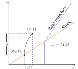
denote the Mach number of the shock wave. The pre- and the post-shock gas properties can be found in Appendix A. Consider any point in the particle-laden domain at a time t, with the position x, denoted as (x, t). The time origin corresponds to the beginning of the cloud interaction, with the shock initially atx = 0. For each point in the (x, t) diagram (seeFig. 1), two configurations are pos-sible, depending on whether the shock wave has already passed the interface (x ≥ Msc t) or not (c being the sound speed in the gas at
rest).
It is possible to calculate the initial position and time of each particle. Letx′be the distance covered by the particle after the inter-action with the shock, andt′ the duration of the interaction. The distance covered by the particle duringt′isx′=x(t′) =x − x0, and
the distance covered by the shock wave isMsct′=Msct − x0.
Know-ing the shock velocity,Vs=Msc, and the gas velocity behind the
shockug, one can deduce from Eq.(4)the velocity as well as the
dis-tance covered by a particlex′as a function of timet′during which it is exposed to the gas of a velocityug,
FIG. 1. Space–time diagram (x, t) of the considered system with xsthe shock position, x′the distance covered by a particle located initially at x
0, and t′the duration of the interaction of the particle with the shock.
⎧ ⎪ ⎪ ⎨ ⎪ ⎪ ⎩ V(t′, τp,ug) =ug(1 −e−t ′/τ p) x(t′, τp,ug) = ∫t ′ 0 V(t, τp,ug)dt = ug(t ′ −τp(1 −e−t ′/τ p)). (6)
The two unknown variables x′ and t′ satisfy the following relations:
{x
′
=x(t′, τp,ug) =x − x0
Msct′=Msct − x0. (7)
By excludingx0from Eq.(7)and substituting the expression forx′
from Eq.(6), one can deduce that ugτp(e−t
′/τ p
−1) +Msc t − x = (Msc − ug)t′. (8)
Solving this equation (cf. Appendix B) gives the following expression: t′(x, t, ug) =τpW ( ugeη Msc − ug )+Msct − ugτp −x Msc − ug , (9) where η =ugτp−Msc t + x τp(Msc − ug) . (10)
The Lambert functionW30is defined implicitly as the solution of the equation α exp(α) = β (seeAppendix B). It is also possible to obtain the Eulerian velocity of the cloudu as
u(x, t, τp,ug) =V(t′(x, t, ug), τp,ug) =ug(1 − exp(−t′(x, t)/τp)).
(11) B. Mean cloud density
Using the conservation of mass, it is possible to determine the global spray characteristics in the post-shock area. If one considers that the timet of the interaction of the shock with the cloud is very large with respect to the response time τp, the first particle distance
covered can be approximated withx(t, τp/t → 0) = ugt. It allows us
to determine the cloud length in the post-shock area as L(t, τp/t → 0, ug) =Msct − x(t, τp/t → 0, ug) = (Msc − ug)t.
(12) Considering that the particles are solid and undeformable, the initial cloud length isMsct and becomes (Msc − ug)t, we deduce that the
post-shock density of the particles τvcan be linked to the pre-shock
density τv,0by
τv(t, τp,ug) =τv,0 Msc
Msc − ug
. (13)
The initial and the post-shock cloud lengths are represented in
Fig. 2(b). Using Eq.(A1), one can obtain τv τv,0 = 1 γ − 1 γ + 1+ 2 γ + 1 1 M2 s . (14)
The evolution of the ratio τv/τv,0 as a function of Ms is given
inFig. 2(a). One can see that when Ms → ∞, τv/τv,0approaches
(γ + 1)/(γ − 1) = 6.0 for air, a value that τv/τv,0 can never exceed.
FIG. 2. Cloud density as a function of the Mach number and the length of cloud in the post-shock area. (a) Evolution ofτv/τv,0as a function of Ms; the dashed blue line represents the asymptotic limit given by (γ + 1)/(γ − 1) with γ = 1.4. (b)
Space–time diagram showing the cloud length pre- and post-shock.
When the inertia of the particles cannot be neglected, one can obtain a mean load rate after the shock passage using Eqs.(6)
and(12),
τv(t, τp,ug) =τv,0 Msc
Msc − ug+ugτtp(1 − exp(−t/τp))
. (15)
Equations(13)and (15)show accumulation of particles after the shock at the contact surface. The evolutions of the particle load rate for different τpand for a fixedMs= 1.1 are given inFig. 3. We can see
that the time necessary to reach the asymptotic value for the particle load rate increases with particle response time as expected.
C. Eulerian cloud density evolution
One more hypothesis is necessary to estimate the Eulerian cloud density evolution. Let us assume that the particles are initially regularly disposed with a mean distance of Δx0between them. The
FIG. 3. Mean load rate evolutions for particles of different τpin air:τp= 3 × 10⁻⁶s (blue solid line),τp= 7.5 × 10⁻⁵s (green solid line),τp= 3 × 10⁻⁴s (red solid line),τp= 1.2 × 10⁻³s (orange solid line),ρp= 103kg/m3, Ms= 1.1, and ug= 55.19 m/s.
FIG. 4. Initial configuration of the shock/particle interaction.
cloud is also initially structured according to a cubic particle shape. The load rate τv,0of this cloud is also the ratio between the volume
taken by the particles and the volume of the gas. The initial organi-zation of the particles and the initial load rate are shown inFig. 4. With such a cubic arrangement, the load rate is
τv,0= πd3p
6 Δx3 0
. (16)
Knowing that the shock propagates along thex-direction, the load rate of the shocked particle-laden region can be
τv(t, τp,ug) =
πd3p
6 Δx2
0Δx(t, τp,ug)
. (17)
Let us consider two neighbor particles on thex-axis at initial posi-tionsx02andx01such asx02−x01 =Δx0. With previous results, it is
possible to estimate the timet′ during which the particles are in the post-shock area. Let us denote Δt = Δx0/Msc, the interval time
taken by the shock to cover the inter-particle distance. The distance between these two particles as a function oft′is
Δx(t′, τp,ug) =x2(t′−Δt, τp,ug) −x1(t′, τp,ug)
= (x02+x(t′−Δt, τp,ug)) − (x01+x(t′, τp,ug)) =Δx0+x(t′−Δt, τp,ug) −x(t′, τp,ug). (18)
Substituting Eqs.(6)and(16)into(18)and according to the defini-tion of Δt and τp, one can deduce
Δx = Δx0(1 − ug Msc )+ugτpexp(−t′/τp) × [exp( √ 18μgτp ρp 3 √ π 6τv,0 1 Mscτp ) −1] . (19)
Dividing Eq.(19)byx0, one can obtain according to Eqs.(16),(17),
and the definition of τp,
τv(t′, τp,ug) τv,0 = ⎡ ⎢ ⎢ ⎢ ⎢ ⎢ ⎢ ⎢ ⎢ ⎢ ⎣ (1 − ug Msc )+ √ ρp 18 μτp 3 √ 6τv,0 π ugτpexp(−t ′ /τp)(exp( √ 18μgτp ρp 3 √ π 6τv,0 1 Mscτp ) −1) ´¹¹¹¹¹¹¹¹¹¹¹¹¹¹¹¹¹¹¹¹¹¹¹¹¹¹¹¹¹¹¹¹¹¹¹¹¹¹¹¹¹¹¹¹¹¹¹¹¹¹¹¹¹¹¹¹¹¹¹¹¹¹¹¹¹¹¹¹¹¹¹¹¹¹¹¹¹¹¹¹¹¹¹¹¹¹¹¹¹¹¹¹¹¹¹¹¹¹¹¹¹¹¹¹¹¹¹¹¹¹¹¹¹¹¹¹¹¹¹¹¹¹¹¹¹¹¹¹¹¹¹¹¹¹¹¹¹¹¹¹¹¹¹¹¹¹¹¹¹¹¹¹¹¹¹¹¹¹¹¹¹¹¹¹¹¹¹¹¹¹¹¹¹¹¹¹¹¹¹¹¹¹¹¹¹¹¹¹¹¹¹¹¹¹¹¹¹¹¹¹¹¹¹¹¹¹¹¹¹¹¹¹¹¹¹¹¹¹¹¹¹¹¹¹¹¹¹¹¹¹¹¹¹¹¹¹¹¹¹¹¹¸¹¹¹¹¹¹¹¹¹¹¹¹¹¹¹¹¹¹¹¹¹¹¹¹¹¹¹¹¹¹¹¹¹¹¹¹¹¹¹¹¹¹¹¹¹¹¹¹¹¹¹¹¹¹¹¹¹¹¹¹¹¹¹¹¹¹¹¹¹¹¹¹¹¹¹¹¹¹¹¹¹¹¹¹¹¹¹¹¹¹¹¹¹¹¹¹¹¹¹¹¹¹¹¹¹¹¹¹¹¹¹¹¹¹¹¹¹¹¹¹¹¹¹¹¹¹¹¹¹¹¹¹¹¹¹¹¹¹¹¹¹¹¹¹¹¹¹¹¹¹¹¹¹¹¹¹¹¹¹¹¹¹¹¹¹¹¹¹¹¹¹¹¹¹¹¹¹¹¹¹¹¹¹¹¹¹¹¹¹¹¹¹¹¹¹¹¹¹¹¹¹¹¹¹¹¹¹¹¹¹¹¹¹¹¹¹¹¹¹¹¹¹¹¹¹¹¹¹¹¹¹¹¹¹¹¹¹¹¹¹¹¶ A ⎤ ⎥ ⎥ ⎥ ⎥ ⎥ ⎥ ⎥ ⎥ ⎥ ⎦ −1 . (20)
Two evident conclusions can be deduced. The term A is always positive and
τv(t′, τp,ug) <τv,0 Msc
Msc − ug
=τv,max, (21)
which is the maximal value of the post-shock density estimated by Eq.(15). In the one-way formalism, we can conclude that for any physical parameters, the maximal density of the cloud can never exceed the mean density that a null-inertia cloud could have. The second point is that, for a very low τp, one can have A → 0. In
this case, the cloud density increases to a constant value τv,max. This
model is applicable for various particle cloud density ratios ρp/ρg,
provided that the gravity of the particles is negligible compared to the drag force.
D. Extension to two-way formalism
With the existence of the particle–gas interaction, the gas veloc-ity decreases due to the conservation of momentum. We can assume that this velocity is reduced by a value ε(ug). The next particle will
relax to a velocity ofug−ε(ug).Figure 5shows the acceleration of
two successive particles by the shock wave in the two-way model. In this case, the load rate will severely increase at the cloud extrem-ity. In addition, the presence of particles can slow down the post-shock gas velocity. It is at the cloud extremity that the particles slipping velocity is the highest. It is also at this location that the gas is most impacted by the presence of particles, and that ε has the
FIG. 5. Sketch of two successive particle motion (a) before and (b) after the shock passage.
highest values. Knowing that the density and the local velocity of the cloud have no analytical solutions, one can only determine the mean characteristics of the cloud after the shock.
First, it is assumed that the Mach number of the transmitted shock takes a constant value equal toMs= 1.1 in the two-way
model-ing. According to numerical simulations, this assumption is justified for small particle volume fractions τv,0<10−3. Our attempt is to obtain the mean post-shock gas velocity ˜ug. Let us consider a volume
elementV inside, which is the particle volume τv,0V. This analysis is
considered in the case where the particles have completely relaxed to the post-shock gas velocity ˜ug. With respect to the kinetic energy
conservation, one can directly deduce
ρgu2gV = ρ′g˜u2gV′+ τv,0V′ρp˜u2g, whereV′≃V (1 − ug Msc ) (22) and ρ′g ρg = (γ + 1) Ms2 2 + (γ − 1) M2 s , (23)
where ρpis the density of the particles. So, we obtain
˜ug= ug √ 1 − ug Msc √ (γ+1)M2 s 2+(γ−1)M2 s + τv,0 ρp ρg . (24)
Taking the mean load rate given by Eq.(15), we have ˜τv=τv,0
Msc
Msc − ˜ug
. (25)
IV. ASSESSMENT OF THE ANALYTICAL MODEL
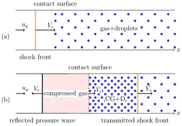
Here, we consider the numerical simulation of the interaction between a shock wave and a gas–particle in the two-phase mixture as illustrated inFig. 6. This is a basic configuration commonly used to study shock wave attenuation particle-laden regions.31A piston moving at a speedugcan generate a shock traveling at a velocityVs
(seeAppendix A).
FIG. 6. Sketch of the shock and contact surface before (a) and after the interaction (b); CG: compressed gas, D: droplets.
TABLE I. Post- and pre-shock gas flow characteristics, Ms= 1.1,ρp/ρg= 553.7.
Gas flow parameters Post-shock Pre-shock
ug(m/s) 58.21 0
ρg(kg/m3) 1.21 1.04
pg(bar) 1.25 1.01
Tg(K) 396 370
The simulations are conducted using an in-home compress-ible Navier–Stokes code named Asphodele, developed in CORIA laboratory Rouen France.32 The Eulerian–Lagrangian approach is used with an Unresolved Discrete Particle Model (UDPM). The space discretization uses a fifth-order WENO (weighted essentially non-oscillatory) scheme with global Lax–Friedrichs splitting.33 A third-order Runge–Kutta method is adopted for time marching. The minimal storage time-advancement scheme34is used to reconstruct the Runge–Kutta method for the temporal resolution. The one-dimensional computational domainL0= 1 m consists of 1000 points,
with 1000 particles initially defined in each elementary cell. The analytical model and the numerical results are compared together in this section. The difference between theoretical and numerical cloud velocities in the one-way formalism is first studied. As illustrated inFig. 6, the shock wave and the contact surface are initially located atx0= 0. These characteristics of the gas in the
pre-and the post-shock domain are given inTable I.
The cloud velocity and the gas velocity are studied for particles with five distinct diameters ranging from nano to micro meters. The particles have a mass density of ρp= 664.4 kg/m3at atmospheric
temperature and pressure corresponding to a given gas (here, we consider cycloheptene C7H16, as an example). Table II gives the
particle diameters and the related equivalent characteristic response time τp. In what follows, we choose the initial pre-shock
proper-ties as characteristic scales such asug ,0, τv,0, andP0. The length of
the calculation domainL0is chosen as the characteristic scale of the
coordinates.
For very small particles (dp= 10 nm anddp= 1 μm), one can
assume that their velocity increases rapidly toward the gas veloc-ity and coincides with it. As a consequence, two areas are noted in
Figs. 7(a)and7(b): the pre-shock area, where both particles and gas are at rest, and the post-shock area, where the gas and the particles velocity are equal toug.
In the case where the particles inertia cannot be neglected, they progressively accelerate to relax toward the gas velocity.
TABLE II. Diameter of particles and corresponding equivalent characteristic response timeτp.
Droplet diameterdp(μm) Response time τp(μs)
0.01 1.575 10−4
1 1.575
10 157.5
20 630
FIG. 7. Eulerian cloud velocity within the one-way formalism. Numerical results (black circle), theoretical model (red solid line), and their maximal value (ug) for different diameters at t = 1.756 ms and
Ms= 1.1, ug ,0= 58.21 m/s,ρp= 664.4 kg/m3; (a) d
p= 10 nm, (b) dp= 1μm, (c) dp= 10μm, and (d) dp= 50μm.
FIG. 8. Droplet volume fraction in the one-way formalism. Numerical results (blue solid line), theoretical model (red solid line), and maximum (τv ,max/τv ,0) for different diameters at t = 1.756 ms,
Ms= 1.1, andρp= 664.4 kg/m3; (a) dp = 10 nm, (b) dp= 1μm, (c) dp= 10μm, and (d) dp= 50μm.
FIG. 9. Comparison between the theoretical model and numerical simulations at 0.2 ms (orange solid line), 0.4 ms (dark blue solid line), 0.6 ms (blue solid line), the-oretical results (red dashed line);τv ,0= 5.2 × 10⁻⁴, dp= 1μm, ρp= 664.4 kg/m3, original contact surface (black dashed line); (a) droplet volume fraction and (b) droplet velocity evolution.
The time necessary for this relaxation process is τp[seeFigs. 7(c)
and 7(d)], which increases with their diameters. A comparison between analytical and numerical results shows a good agreement in terms of gas and particle velocities (seeFig. 7).
Figure 8shows comparisons of the temporal evolutions of the cloud density τvbetween the numerical simulations and the
analyt-ical model given by Eq.(21)for particle cloud of different diame-ters. Different from the continuous solution given by the analytical model, the numerical results show some oscillatory behavior as a result of the random repartition of particles in the Lagrangian for-malism used in the Navier–Stokes code. The mean cloud density is seen to be close to the analytical prediction, which is limited by the maximal cloud density obtained by Eq.(21).
The small particles respond immediately to the gas flow [see
Figs. 8(a)and 8(b)], while the larger ones accelerate progressively [see Figs. 8(c) and 8(d)]. It can be concluded that the relation-ship established before in a one-way formalism is validated by the numerical simulations.
The extended two-way theoretical model is studied by com-parison with the numerical simulations using two-way formalism as given inFig. 9. The volume fraction evolution of the particles is shown inFig. 9(a)for particles of diameter 1 μm. The maximal value for the volume fraction increases from 5.2 × 10⁻⁴to 6.08 × 10⁻⁴. Similarly, Fig. 9(b) shows the comparison of particle velocities, which increases sharply toward a maximal value that is lower than the initial post-shock gas velocity. The theoretical particle velocity is slightly smaller than the calculation, which results in a lower estima-tion of the volume fracestima-tion as shown inFig. 9(a). In fact, Eq.(24)can only give a global estimation of the real particle velocity. The relative error of the volume fraction is 2% in the case of 1 μm.
V. NUMERICAL RESULTS
A. One-way vs two-way simulations
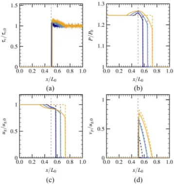
In this section, the comparison of numerical results using one-way and two-one-way formalisms is given.Figure 10(a)shows the evo-lution of volume fraction of particles in the computational domain
FIG. 10. Comparison one-way/two-way for different time instants. One-way on 0.2 ms (dark blue dashed line), 0.4 ms (blue dashed line), and 0.6 ms (orange dashed line) and two-way on 0.2 ms (dark blue solid line), on 0.4 ms (blue solid line), 0.6 ms (orange solid line);τv ,0= 5.2 × 10⁻⁴, dp= 10μm, ρp= 103kg/m3, original contact surface (black dashed line); (a) droplet volume fraction, (b) gas pressure, (c) gas velocity, and (d) droplet velocity.
fort = 200–600 μs. It can be seen that the volume fraction of the particles increases after the passage of the shock. The amplification of the high volume fraction is around 1.1 times the original volume fraction. The interface of the pure gas and the particle-laden domain is pushed downstream of the gas flow. The mass density of particles takes the value of ρp= 103kg/m3in the following simulations.
Figure 10(b)shows the pressure evolution in the computational domain. Results of the two-way simulations are highlighted by solid lines, while the corresponding one-way simulations are depicted by dashed lines. First, as a result of the attenuation effects of particles, one can notice that the pressure of the post-shock gas is lower than the one-way coupling. This shows that the strength of the shock is decreased due to the presence of particles. Second, the reflec-tion pressure waves are seen only in the two-way simulareflec-tion. The maximal value for the post-shock pressure is 1.27 bar located at the interface of the two domains. Moreover, the reflection pressure wave propagates at a velocity lower than the original shock wave.
Figure 10(c)shows the evolution of the gas velocity. The one-way simulation indicates that there is no change in the post-shock gas velocity, while this quantity is much reduced in the two-way method, with a maximal velocity of gas smaller than 55 m/s. An effective change of particle velocity can be seen in Fig. 10(d)for the two-way simulation. After the passage of the shock, the parti-cle velocities are smaller in the two-way simulation compared to the one-way case.
The comparison indicates that the two-way formalism should be taken into account to better describe the interaction process between the shock wave and the particle cloud.
B. Effects of particle response time
It is noted that several characteristics of the cloud such as the characteristic response time τpand the volume fraction of particle
τv,0can have important effects on the interaction mechanism. These
effects are studied numerically in this part.
Figure 11(a)shows the gas velocity evolution after the passage of the shock wave through the cloud. Different particle sizes are sim-ulated to elucidate the effect of the response time. The interaction between the particles and the shock can effectively decelerate the post-shock gas velocity. For example, the velocity is reduced from 55 m/s to 50 m/s for particles having a diameter of 1 μm and a volume fraction of τv,0= 5.2 × 10⁻⁴. The small particles respond
rapidly to the shock wave, and give a piece-wise structure of the gas properties during the shock–particle interaction. The larger parti-cles are more difficult to accelerate; thus, they reduce gradually the gas velocity.
The evolution of the particle volume fraction after the passage of the shock is given inFig. 11(b). One can see that the small particles can give an upper bound of cloud density for the larger ones, which confirms the statement deduced from Eq.(21)through an analytical model.
C. Effect of particle volume fraction
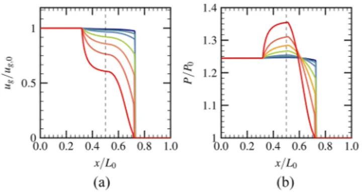
The last section concerns the study of the effect of the particle volume fraction.Figure 12(a)shows the gas velocity evolution for different particle volume fractions. The reduction of the gas velocity is much reinforced by the increase in the particle volume fraction. However, the reflected and the transmitted wave velocities seem to be independent of the volume fraction. For a very dense cloud, where τv,0= 5 × 10⁻³, the post-shock gas velocity reduces to zero at 600 μs,
which means that there is no more transmitted pressure wave.
FIG. 11. Evolutions of flow parameters for different particle diameters: dp= 1μm (dark blue solid line), dp= 2μm (dark green solid line), dp= 4μm (blue solid line), dp= 6μm (green solid line), dp= 8μm (orange solid line), dp= 10μm (red solid line); t = 600μs, τv ,0= 5.2 × 10⁻⁴, Ms= 1.1,ρp= 103kg/m3, original contact surface (black dashed line); (a) gas velocity evolution, (b) droplet velocity evolution.
FIG. 12. Evolutions of flow parameters for different particle volume fractions:
τv ,0= 5 × 10⁻⁵(dark blue solid line),τv ,0= 1 × 10⁻⁴(dark green solid line), τv ,0= 2 × 10⁻⁴(blue solid line),τv ,0= 5 × 10⁻⁴(green solid line),τv ,0= 1 × 10⁻³ (orange solid line),τv ,0= 2 × 10⁻³(dark orange solid line),τv ,0= 5 × 10⁻³(red solid line); t = 600μs, dp= 10μm, Ms= 1.1,ρp= 103kg/m3, original contact surface (black solid line); (a) gas velocity and (b) gas pressure.
Figure 12(b)gives the pressure evolution after the interaction between a shock and the cloud of diameterdp= 10 μm. One can
notice that the particles of volume fraction τv,0 = 5 × 10⁻⁵ have
less influence on the pressure evolution. A higher volume fraction τv,0= 5 × 10⁻³shows an evident pressure increase at the interface
between the pure gas and the particle-laden region. It seems that the transmitted pressure is completely attenuated at aroundx = 0.75 m in this case. The reflection pressure wave can be noted for all particle volume fractions, and the velocity of the reflected wave seems to be very close.
The comparison shows that the particle volume fraction can enhance the reflection pressure value and play an important role in the attenuation of the transmitted shock.
VI. CONCLUSIONS
An analytical model is developed to study the cloud topology after the passage of a shock wave in the framework of a one-way interaction formalism. Special attention is made to the momen-tum exchange between the shock and particles in order to elucidate the dynamic aspects of the shock–cloud interaction mechanisms. The assessment of the model is conducted through a compari-son with numerical simulations performed using a high accuracy Navier–Stokes solver.
The extension of the one-way analytical model to the two-way formulation is proposed and compared to the numerical two-way simulations. The two-way theoretical model shows less accuracy than the one-way modeling, but still remains predictable in the scope of this study.
The necessity of using the two-way formalism in the numer-ical simulation of the shock–cloud interaction is discussed. Vari-ous mechanisms such as shock reflection and attenuation can be observed in the two-way simulations, which are neglected in the one-way formalism.
Small particles of diameterO(1) μm are more sensitive to the drag of the post-shock gas and the present piece-wise structures of
the shock–cloud interaction. An important shock attenuation effect is noticed for the particle cloud of high volume fractionsO(10−3).
More studies can be performed considering the two- or three-dimensional shock–spray interactions to study the role of the trans-verse waves on the spray dispersion. The polydispersion of the cloud particles as well as the secondary breakup of the water spray can also be included in the simulations to improve the spray dispersion modeling.
ACKNOWLEDGMENTS
The authors gratefully acknowledge the financial support from Electricité de France (EDF) within the framework of the Generation II and III reactor research program.
APPENDIX A: CHARACTERISTICS OF THE PLANAR SHOCK
A planar shock wave can be generated by a piston as shown inFig. 13. The piston starts moving att = 0 with a velocity Vp,
generating a shock wave with a velocityVs. Two areas are divided
by the shock wave: the post- (1) and the pre-shock area (2). Given the sound speed in the pre-shock area,c2, one can obtain the piston
velocity,Vp, by the following relation:
2 γ + 1 M2s−1 Ms = Vp c2 ; Vs=Msc2. (A1)
The post-shock gaseous flow is assumed to have the same veloc-ity as that of the piston. Analytical solutions are available for the relationship of the pre- and post-shock thermodynamic quantities,35
p1 p0 =Γ1(Ms, γ), T1 T0 =Γ1(Ms, γ)Γ2(Ms, γ) M2 s , ρ1 ρ0 =p1 p0 T0 T1 , (A2) where Γ1(Ms, γ) = 2 γ + 1(γM 2 s−γ − 1 2 ), Γ2(Ms, γ) = 2 γ + 1(1 + γ − 1 2 M 2 s). (A3) APPENDIX B: RESOLUTION OF EQ.(8)
Equation(8)has the form t′(Msc − ug) =ugτp(exp(−
t′ τp
) −1) +Msct − x, (B1)
FIG. 13. Shock wave generation in a piston tube.
which can be written, by the arrangement of terms, as ⎡ ⎢ ⎢ ⎢ ⎢ ⎢ ⎢ ⎢ ⎢ ⎣ t′ τp − Msc t − x − ugτp τp(Msc − ug) ´¹¹¹¹¹¹¹¹¹¹¹¹¹¹¹¹¹¹¹¹¹¹¹¹¹¹¹¹¹¹¹¹¹¹¹¹¹¹¹¹¹¹¹¹¹¹¹¹¹¹¹¹¹¹¹¹¹¹¹¸¹¹¹¹¹¹¹¹¹¹¹¹¹¹¹¹¹¹¹¹¹¹¹¹¹¹¹¹¹¹¹¹¹¹¹¹¹¹¹¹¹¹¹¹¹¹¹¹¹¹¹¹¹¹¹¹¹¹¹¶ α ⎤ ⎥ ⎥ ⎥ ⎥ ⎥ ⎥ ⎥ ⎥ ⎦ exp ⎛ ⎜ ⎜ ⎜ ⎜ ⎝ α ³¹¹¹¹¹¹¹¹¹¹¹¹¹¹¹¹¹¹¹¹¹¹¹¹¹¹¹¹¹¹¹¹¹¹¹¹¹¹¹¹¹¹¹¹¹¹¹¹¹¹¹¹¹¹¹¹¹¹¹·¹¹¹¹¹¹¹¹¹¹¹¹¹¹¹¹¹¹¹¹¹¹¹¹¹¹¹¹¹¹¹¹¹¹¹¹¹¹¹¹¹¹¹¹¹¹¹¹¹¹¹¹¹¹¹¹¹¹¹µ t′ τp − Msc t − x − ugτp τp(Msc − ug) ⎞ ⎟ ⎟ ⎟ ⎟ ⎠ = ug Msc − ug exp(−Msc t − x − ugτp τp(Msc − ug) ) ´¹¹¹¹¹¹¹¹¹¹¹¹¹¹¹¹¹¹¹¹¹¹¹¹¹¹¹¹¹¹¹¹¹¹¹¹¹¹¹¹¹¹¹¹¹¹¹¹¹¹¹¹¹¹¹¹¹¹¹¹¹¹¹¹¹¹¹¹¹¹¹¹¹¹¹¹¹¹¹¹¹¹¹¹¹¹¹¹¹¹¹¹¹¹¹¹¹¹¹¹¹¹¹¹¸¹¹¹¹¹¹¹¹¹¹¹¹¹¹¹¹¹¹¹¹¹¹¹¹¹¹¹¹¹¹¹¹¹¹¹¹¹¹¹¹¹¹¹¹¹¹¹¹¹¹¹¹¹¹¹¹¹¹¹¹¹¹¹¹¹¹¹¹¹¹¹¹¹¹¹¹¹¹¹¹¹¹¹¹¹¹¹¹¹¹¹¹¹¹¹¹¹¹¹¹¹¹¹¹¶ β . (B2)
The previous equation can also be written as α exp(α) = β. We obtain, thanks to theW Lambert function,30 α = W(β). As a consequence, one can obtain
t′=τpW[ ug Msc − ug exp(−Msc t − x − ugτp τp(Msc − ug) )]+Msc t − x − ugτp Msc − ug . (B3) REFERENCES 1
G. Carrier, “Shock waves in a dusty gas,”J. Fluid Mech.4, 376–382 (1958). 2
G. Jourdan, L. Biamino, C. Mariani, C. Blanchot, E. Daniel, J. Massoni, L. Houas, R. Tosello, and D. Praguine, “Attenuation of a shock wave passing through a cloud of water droplets,”Shock Waves20, 285–296 (2010).
3
T. Theofanous, V. Mitkin, and C.-H. Chang, “The dynamics of dense particle clouds subjected to shock waves. Part 1. Experiments and scaling laws,”J. Fluid Mech.792, 658–681 (2016).
4
J. Kersey, E. Loth, and D. Lankford, “Effect of evaporating droplets on shock waves,”AIAA J.48, 1975–1986 (2010).
5O. Williams, T. Nguyen, A.-M. Schreyer, and A. Smits, “Particle response anal-ysis for particle image velocimetry in supersonic flows,”Phys. Fluids27, 076101 (2015).
6G. Rudinger, “Some properties of shock relaxation in gas flows carrying small particles,”Phys. Fluids7, 658–663 (1964).
7
M. Olim, G. Ben-Dor, M. Mond, and O. Igra, “A general attenuation law of mod-erate planar shock waves propagating into dusty gases with relatively high loading ratios of solid particles,”Fluid Dyn. Res.6, 185–199 (1990).
8
J. Geng, A. V. de Ven, Q. Yu, F. Zhang, and H. Grönig, “Interaction of a shock wave with a two-phase interface,”Shock Waves3, 193–199 (1994).
9Y. Ling, L. Wagner, S. Beresh, S. Kearney, and S. Balachandar, “Interaction of a planar shock wave with a dense particle curtain: Modeling and experiments,” Phys. Fluids24, 113301 (2012).
10J. McFarland, W. Black, J. Dahal, and B. Morgan, “Computational study of the shock driven instability of a multiphase particle-gas system,”Phys. Fluids28, 024105 (2016).
11B. Gelfand, “Droplet break-up phenomena in flows with velocity lag,”Prog. Energy Combust. Sci.22, 201–265 (1996).
12
A. Hadjadj and O. Sadot, “Shock and blast waves mitigation,”Shock Waves23, 1–4 (2013).
13A. Britan, H. Shapiro, M. Liverts, G. Ben-Dor, A. Chinnayya, and A. Hadjadj, “Macro-mechanical modelling of blast wave mitigation in foams. Part I: Review of available experiments and models,”Shock Waves23, 5–23 (2013).
14E. D. Prete, A. Chinnayya, L. Domergue, A. Hadjadj, and J.-F. Haas, “Blast wave mitigation by dry aqueous foams,”Shock Waves23, 39–53 (2013).
15
G. Jourdan, C. Mariani, L. Houas, A. Chinnayya, A. Hadjadj, E. D. Prete, J.-F. Haas, N. Rambert, D. Counilh, and S. Faure, “Analysis of shock-wave propa-gation in aqueous foams using shock tube experiments,”Phys. Fluids27, 056101 (2015).
16A. Foissac, J. Malet, M. Vetrano, J. Buchlin, S. Mimouni, F. Feuilleboiset al., “Droplet size and velocity measurements at the outlet of a hollow cone spray nozzle,”Atomization Sprays21, 893–905 (2011).
17
G. Thomas, “On the conditions required for explosion mitigation by water sprays,”Process Saf. Environ.78, 339–354 (2000).
18
G. Gai, S. Kudriakov, A. Hadjadj, E. Studer, and O. Thomine, “Modeling pres-sure loads during a premixed hydrogen combustion in the presence of water spray,”Int. J. Hydrogen Energy44, 4592–4607 (2019).
19
T. Hanson, D. Davidson, and R. Hanson, “Shock-induced behavior in micron-sized water aerosols,”Phys. Fluids19, 056104 (2007).
20
A. Chauvin, G. Jourdan, E. Daniel, L. Houas, and R. Tosello, “Experimental investigation of the propagation of a planar shock wave through a two-phase gas-liquid medium,”Phys. Fluids23, 113301 (2011).
21
M. Pilch and C. Erdman, “Use of breakup time data and velocity history data to predict the maximum size of stable fragments for acceleration-induced breakup of a liquid drop,”Int. J. Multiphase Flow13, 741–757 (1987).
22D. Guildenbecher, C. Lopez-Rivera, and P. Sojka, “Secondary atomization,” Exp. Fluids46, 371–402 (2009).
23
Y. Ling, A. Haselbacher, and S. Balachandar, “Importance of unsteady contri-butions to force and heating for particles in compressible flows. Part 2: Applica-tion to particle dispersal by blast waves,”Int. J. Multiphase Flow37, 1013–1025 (2011).
24Y. Mehta, T. Jackson, J. Zhang, and S. Balachandar, “Numerical investigation of shock interaction with one-dimensional transverse array of particles in air,” J. Appl. Phys.119, 104901 (2016).
25J. Dahal and J. McFarland, “A numerical method for shock driven multiphase flow with evaporating particles,”J. Comput. Phys.344, 210–233 (2017).
26
J. Wagner, S. Beresh, S. Kearney, W. Trott, J. Castaneda, B. Pruett, and M. Baer, “A multiphase shock tube for shock wave interactions with dense particle fields,” Exp. Fluids52, 1507–1517 (2012).
27
Y. Sugiyama, H. Ando, K. Shimura, and A. Matsuo, “Numerical investigation of the interaction between a shock wave and a particle cloud curtain using a CFD– DEM model,”Shock Waves29, 499–510 (2018).
28
K. Wingerden and B. Wilkins, “The influence of water sprays on gas explosions. Part 2: Mitigation,”J. Loss Prev. Process Ind.8, 61–70 (1995).
29S. Elghobashi, “An updated classification map of particle-laden turbulent flows,” inIUTAM Symposium on Computational Approaches to Multiphase Flow (Springer, 2006), Vol. 81, pp. 3–10.
30R. Corless, G. Gonnet, D. Hare, D. Jeffrey, and D. Knuth, “On the Lambert W function,”Adv. Comput. Math.5, 329–359 (1996).
31
E. Chang and K. Kailasanath, “Shock wave interactions with particles and liquid fuel droplets,”Shock Waves12, 333–341 (2003).
32O. Thomine, “Development of multi-scale methods for the numerical sim-ulation of biphasic reactive flows,” Ph.D. thesis, University of Rouen, France, 2011.
33G.-S. Jiang and C.-W. Shu, “Efficient implementation of weighted ENO schemes,”J. Comput. Phys.126, 202–228 (1996).
34
A. Wray, “Minimal storage time-advancement schemes for spectral methods,” Technical Report No. MS 202, NASA Ames Research Center, 1991.
35F. White, Fluid Mechanics, McGraw-Hill Series in Mechanical Engineering (McGraw-Hill, 2011).