Distributional models of ocean carbon export

Distributional models of ocean carbon export

Brendan Barry

Submitted to the Joint Program in Physical Oceanography in partial fulfillment of the requirements for the degree of

Doctor of Philosophy at the

MASSACHUSETTS INSTITUTE OF TECHNOLOGY and the

WOODS HOLE OCEANOGRAPHIC INSTITUTION February 2019

@2019

The author hereby grants to MIT and WHOI permission to reproduce and to distribute publicly paper and electronic copies of this thesis document in whole or in

part in any medium now known or hereafter created.

Signature redacte

Signature

... ... ... .... ...

Join Program in h a ceanograp

assachuset stitut of T o ogy

ods Ho ceanographic Institution

redacted

C ertified b y ... ... Michael J. Follows Professor of Earth, Atmospheric, and Planetary Sciences Massachusetts Institute of Technology Thesis Supervisor A ccepted by ... OF TECHNOLOGY

FEB

0

6 2019

LIBRARIES

ARCHIVES

Signature redacted

Chairman, Joint Committee for Physical Oceanography Massachusetts Institute of Technology Woods Hole Oceanographic Institution

Distributional models of ocean carbon export by

Brendan Barry

Submitted to the Joint Program in Physical Oceanography Massachusetts Institute of Technology

& Woods Hole Oceanographic Institution on December 12, 2018, in partial fulfillment of the

requirements for the degree of Doctor of Philosophy

Abstract

Each year, surface ocean ecosystems export sinking particles containing gigatons of carbon into the ocean's interior. This particle flux connects the entire ocean microbiome and consti-tutes a fundamental aspect of marine microbial ecology and biogeochemical cycles. Particle flux is also variable and intricately complex, impeding its mechanistic or quantitative de-scription. In this thesis we pair compilations of available data with novel mathematical models to explore the relationships between particle flux and other key variables - temper-ature, net primary production, and depth. Particular use is made of (probability) distribu-tional descriptions of quantities that are known to vary appreciably. First, using established thermodynamic dependencies for primary production and respiration, a simple mechanistic model is developed relating export efficiency (i.e. the fraction of primary production that is exported out of the surface ocean via particle flux) to temperature. The model accounts for the observed variability in export efficiency due to temperature without idealizing out the remaining variability that evinces particle flux's complexity. This model is then used to esti-mate the metabolically-driven change in average export efficiency over the era of long-term global sea surface temperature records, and it is shown that the underlying mechanism may help explain glacial-interglacial atmospheric carbon dioxide drawdown. The relationship between particle flux and net primary production is then explored. Given that these are inextricable but highly variable and measured on different effective scales, it is hypothesized that a quantitative relationship emerges between collections of the two measurements - i.e. that they can be related not measurement-by-measurement but rather via their probability distributions. It is shown that on large spatial or temporal scales both are consistent with lognormal distributions, as expected if each is considered as the collective result of many subprocesses. A relationship is then derived between the log-moments of their distributions and agreement is found between independent estimates of this relationship, suggesting that upper ocean particle flux is predictable from net primary production on large spatiotempo-ral scales. Finally, the attenuation of particle flux with depth is explored. It is shown that while several particle flux-versus-depth models capture observations equivalently, these carry very different implications mechanistically and for magnitudes of export out of the surface ocean. A model is then proposed for this relationship that accounts for measurements of both the flux profile and of the settling velocity distribution of particulate matter, and is thus more consistent with and constrained by empirical knowledge. Possible future applica-tions of these models are discussed, as well as how they could be tested and/or constrained observationally.

Thesis Supervisor: Michael J. Follows

Title: Professor of Earth, Atmospheric, and Planetary Sciences Massachusetts Institute of Technology

Acknowledgments

Despite the premise that a thesis represents individual effort, to get here has taken a large and diverse village, each member of which I am grateful for and indebted to, for support, assistance, patience, encouragement, enthusiasm, challenge, trust, and all other phenomena that comprise life and inquiry. I thank my family, friends, labmates, classmates, and col-leagues - those within WHOI and MIT, at the University of Chicago, and those that make up my larger scientific community - for everything. Any and all of you, if you are reading this: thank you for everything. I thank my thesis committee - Ken Buesseler, Raf Ferrari, Melissa Omand, and Dan Rothman - and my thesis chair, Andrew Babbin, for their per-spectives, conversations, and precious time. I thank the many people who continue to make possible all of what goes on at MIT, WHOI, and in the Joint Program. I thank Geoff Lynn for designing Figure 1-1. I thank the Massachusetts Institute of Technology, the National Science Foundation, and the National Aeronautics and Space Administration for financial support. I thank Chris Follett for being a tremendous and generous font of wisdom, both scientific and otherwise, from whom I have learned so much. It would be remiss of me not to extend a particularly heartfelt thanks to Kelsey Bisson for every moment of our friendship and colleagueship, which has always been nurturing, inspiring, and joyous. Finally, it is a deep and true pleasure, which even as I write this elicits tears, to thank my advisor, mentor, and friend, Mick Follows, for putting up with me over these years - and for always being exactly what I needed you to be.

Contents

1 Introduction 19

2 Temperature and export efficiency

2.1 On the temperature dependence of oceanic export efficiency 2.1.1 O verview . . . . 2.1.2 Introduction . . . . 2.1.3 Temperature vs. export efficiency: Model and Data . 2.1.4 Temperature shifts measurements' distribution . . . 2.1.5 D iscussion . . . . 2.2 How have recent temperature changes affected the efficiency ical carbon export? . . . . 2.2.1 O verview . . . . 2.2.2 Introduction . . . . 2.2.3 A metabolic model of export efficiency . . . . 2.2.4 2.2.5 2.2.6 2.2.7 33 . . . 33 . . . 33 . . . 34 . . . 35 . . . 38 . . . 42 of ocean biolog-. biolog-. biolog-. biolog-. biolog-. biolog-. biolog-. biolog-. biolog-. biolog-. 43 . . . 43 . . . 43 . . . 44 Global estimates of multidecadal change in export efficiency . . . . . C onclusion . . . . Sensitivity of atmospheric CO2 to export efficiency at equilibrium . .

Statistical details and sensitivity . . . . 3 Primary production and export

3.1 Can Rates of Ocean Primary Production and Biological Carbon Export Be Related Through Their Probability Distributions? . . . . 3.1.1 O verview . . . . 3.1.2 Introduction . . . . 3.1.3 Theory: the lognormal distribution as a null model . . . .

46 50 51 53 57 57 57 58 62 7

.

.

.

3.1.4 3.1.5 3.1.6 3.1.7 3.1.8 3.1.9 3.1.10 3.1.11 3.1.12 3.1.13 3.1.14 3.1.15 3.1.16 3.1.17 3.1.18 3.1.19 3.1.20

Theory: relating export and production by their distributions' moments Compilation of production measurements . . . . Subregions of production measurements . . . . Compilation of export measurements . . . . Statistical m ethods . . . . Production and export are log normally distributed . . . . Log-Moments of subregions' production distributions sort predictably. Export scales sublinearly with production . . . . What Are the uses and requirements of a more complete theory? . . . Can the probabilistic approach developed here be used to test models? What about the spatiotemporal structure of the surface ocean? . . . . C onclusion . . . . Re-examining efficiency-production relationships . . . . Convergence of the Central Limit Theorem . . . . Derivation of log-moment relationships . . . . Lower cutoff for production measurements . . . . Kuiper's statistic and other cumulative distribution function statistics 4 Depth and particulate organic carbon flux

4.1 Particle flux parameterizations: quantitative and mechanistic similarities and differences . . . . 64 65 66 68 69 70 70 74 77 79 80 81 81 85 86 87 89 91 91 Overview . . . . Introduction . . . .

Several mechanistic particle flux attenuation models .

Large differences in export estimates . . . . Quantitative indistinguishability . . . .

Conclusion . . . .

Derivations . . . . Flux profiles . . . . Euphotic and mixed layer depth climatologies . . . . . Normalizations . . . . Statistical routine . . . . . . . 91 . . . 92 . . . 93 . . . 94 . . . 97 . . . 98 . . . 99 . . . 104 . . . 104 . . . 104 . . . 106 8 4.1.1 4.1.2 4.1.3 4.1.4 4.1.5 4.1.6 4.1.7 4.1.8 4.1.9 4.1.10 4.1.11

4.2 Distributional model for particle flux attenuation . . . 112

4.2.1 Overview . . . 112

4.2.2 Particle flux complexity . . . 113

4.2.3 Settling velocity distribution data . . . 115

4.2.4 Distributional model . . . 118

4.2.5 Fit to settling velocity distribution data . . . 121

4.2.6 Fit to flux-depth data . . . 122

4.2.7 Discussion . . . 127

5 Summary and future directions 131

List of Figures

1-1 Illustration of the global carbon cycle. . . . 21 1-2 Simplified illustration of the carbon cycle, taken from Figure S2 of [Cael et al.,

20 17]. . . . 22 1-3 Illustration of the pathways of the biological pump, taken from Figure 4 of

[Siegel and Others, 2016]. . . . 26

2-1 Temperature sensitivity for phytoplankton and copepod growth rates, adapted from (a) Eppley [Eppley, 19721 and (b) Huntley and Lopez [Huntley and Lopez, 1992]. The temperature scaling prefactor is larger for the copepods, the key thermodynamic relation that drives this model. Another key dif-ference is that copepod growth clusters along, while phytoplankton growth lies under, their respective curves; copepod growth appears to deviate sig-nificantly from this curve near T = 24'C. These predictions from the above pictured original data sets have been additionally tested and verified in, e.g., Rose and Caron [Rose and Caron, 2007]. Note the x axes of each subplot cover different limits. The prefactor is the value which multiplies temperature in

the expressions p

cx

Ax

2-2 Model prediction for maximum export efficiency as a function of temperature, compared with data from sources described in Methods. The four points enclosed by diamonds were those taken to fix parameter a = .24. The model agrees well with data in its applicable temperature range - vertical dashed line indicates the cutoff at 24'C observable in Huntley and Lopez [Huntley and Lopez, 1992] and Rose and Caron [Rose and Caron, 2007]. Remaining dashed lines indicate possible extrapolations of the model prediction above 240C. ... ... 40

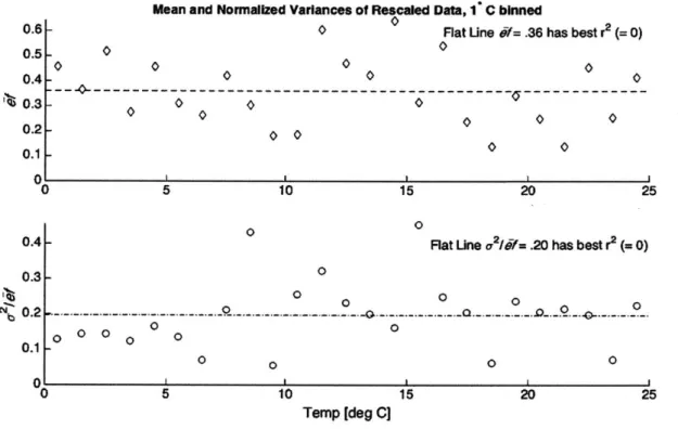
2-3 Mean and normalized variance of the data after being binned at width 1C and rescaled by predicted maximum export efficiency. Binned values are best explained by a constant line; the best fit regression line computed with ordinary least squares has a negative adjusted r2; thus, after the model's prediction for temperature dependence has been removed, no variation in the binned values can be explained by temperature. . . . 41

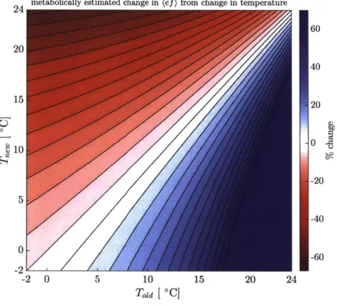
2-4 Percent change in (ef) after a temperature change, as estimated by MM (see Eq. (2.9)), as a function of the initial and final temperatures (Told and Tne). Contours are spaced at 5%. . . . 47

2-5 Percent change in (ef) from 1982-2014, as estimated by MM, as a function of latitude, for different data products. Color corresponds to SST product and line type to P product. Black curve is the average across the SST-P pairs. . . 50

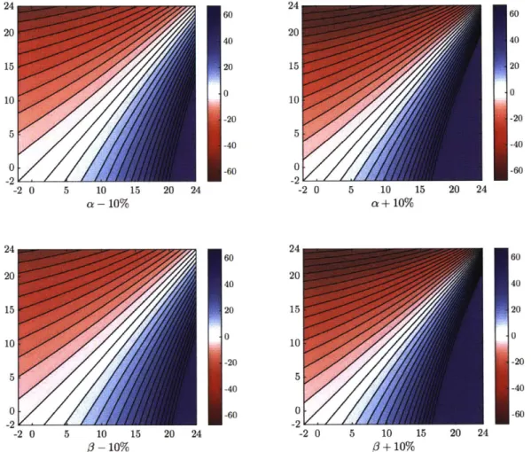
2-6 a-d) As in Figure 2-4, except for a or 3 are changed by 10% in each case, as noted below each subfigure. The overall structure of ef changes is similar, but the magnitude of ef changes for a given temperature change increases with both a and 3. . . . 54

3-1 Scatterplot of particulate organic carbon flux (f) at 100m and depth-integrated net primary production by phytoplankton (P) data from [Maiti et al., 2013]. Notice the lack of a clear correlation between the two. Metrics reported are from Pearson's correlation: The fraction of variance of explained (R2) and the p value of the correlation. Compare to Figure 3-10. . . . 59

3-2 Schematic of approach: p and

f

3-3 Top: Locations of p samples > 0.5 mug C L- 1 day-1 from the compilation

by [Buitenhuis et al., 2013]; compare to their Figure 2a. The solid black

boundary line denotes the separation of data into ocean basins (Section 3.1.6). The time series are indicated by crosses. Middle: Locations of

f

mg C m- 2 day1 from the compilation. The time series are indicated by crosses. Bottom: Map of biomes into which p and

f

num-ber of samples included in the PDF, which excludes data from HOT, BATS, CARIACO, as well as data below the 10% of peak height threshold < 0.5 pg

C L- 1 day-1. Green curve is the probability density function of the lognor-mal which minimizes the Kuiper statistic as compared to the data. Bottom: PDF of global

f

of samples included in the PDF, which excludes data from HOT, BATS, and CARIACO time series, as well as data below the 10% of peak height threshold of 3.6 mg C m-2 day-1. Green curve is the probability density function of the lognormal which minimizes the Kuiper statistic as compared to the data. HOT = Hawaii Ocean Time; BATS = Bermuda Atlantic Time series Study; CARIACO = CArbon Retention In A Colored Ocean time series; PDF = probability density function. . . . 71

3-5 Probability density functions (PDFs) of p data for different subregions. In each case the green curves are the PDF of the lognormal which minimizes the

Kuiper statistic as compared to the data. (p, a) is plotted in Figure 3-6. . . . 72 3-6 Log-moments for each of the p subregions. Error bars are 95% confidence

intervals estimated from bootstrapping; contours are lines of constant mean for a lognormal distribution, equal to exp(p + _1 ) . . . . . . . 73 3-7 Histograms of time series' p and

f

f

in Figure 3-8; p data for the biomes are plotted in Figure 3-5. . . . . 76

3-8 pf versus pp for the three time series, the three biomes, and the global ocean. Dotted blue line is the estimated line from the regression on the biomes (pf =

aQbp

time series (pf = atap + Ct); parameter estimates from the regressions are reported in the top-left of the figure, along with their estimated standard errors. Solid black lines represent 95% bootstrap confidence intervals. The global distributions' log-means (yellow) are not included in the regressions that produce the dashed lines. Inset:

of

op

uf=

ap;

o's

3-9 Illustration of spurious relationships. a) scatterplot of x and y, two uncorre-lated random variables sampled from a uniform distribution (n = 200). b) y/x plotted against x (dashed line is 1/x; compare to Maiti et al. [Maiti et al., 2013]). c) X and Y are binned averages of x and y, into five bins; dashed line is two-parameter fit (Y = 0.45; X-0 08; r2 = 0.99); compare to Laws et al. [Laws et al., 2000a]. 1/8 random sample sets will have a monotonic relationship such as the one seen here if binned into five bins (2-4 = 1/16 will be monotonically increasing and 1/16 will be monotonically decreasing; this number increases rapidly even in response to very weak correlations, e.g.

p = 0.01). . . . 83

3-10 P and ef data from Laws et al. [Laws et al., 2000a], originally compiled by Dunne et al. [Dunne et al., 2005]. Metrics reported are from Pearson's correlation: the fraction of variance of explained (R2) and the P-value of the correlation. . . . 84

3-11 PDF of sums of triplets drawn from the unit uniform distribution, with normal distribution overlaid, illustrating the rapid convergence of the Central Limit T heorem . . . . 85

3-12 Identification of the lower threshold for p samples considered. a) Bars are PDF of measurements of p > 0; dashed black line (for both panels) is the threshold identified at 0.5 pg C L- 1 d- 1, or -10% of the peak in the log-transformed distribution. Green line is a lognormal probability distribution function above the threshold. b) Bars are the relative residual error of the lognormal distribution shown in panel (a). . . . 88

4-1 A: Seven models from the text fit to mesopelagic data from Figure 5 of Martin et al. [Martin et al., 1987b] (their 'Open Ocean Composite') and extended upwards to 50m depth. Goodness-of-fits are very similar, but the power-law model overestimates particulate organic carbon (POC) flux at 50m by 132% relative to the exponential model. Inset shows attenuation (I ) dif-ferences are even more pronounced. Attenuation for the exponential model coincides with most others around -400m. B: Maximum tolerable root-mean-square error (RMSE) to distinguish models based on data from (A) with 90% confidence, estimated using a bootstrap method (see text for details). Row corresponds to 'true' model (from which data are assumed to be generated) and column corresponds to 'false' model (to be rejected). RMSEs are small relative to those in (A), indicating differences in goodness-of-fits between the models are not statistically significant. C: Ratio of power-law-model- and exponential-model-estimated POC flux at euphotic layer and mixed layer depths from the profiles in the data compilation as a function of extrapo-lation distance. Grey shading shows nominal 25% measurement uncertainty. Note the y-axis is logarithmic. The power-law model systematically and sub-stantially overestimates relative to the exponential model (as well as the other models - see Section 4.1.10). For 29 profiles, fp(MLD)/fe(MLD) > 10 (not show n ).) . . . 95

4-2 A map of data locations with histograms of data properties. POC flux is reported in mg C m- 2 d-1. . . . 103

4-3 Cumulative distribution function of fixed-parameter vs. fit-parameter nor-malizations. Horizontal lines indicate the fraction of profiles in each case where the fixed-parameter normalization underestimates relative to the fit-parameter normalization. That these are all close to 0.5 indicates that the approximations of 500 m for

e

rejecting the 'false' (column) model in favor of the 'true' (row) one, from applying the statistical routine illustrated (a) to an artificial profile with ob-servations at z = [125, 250, 500, 1000, 2000, 4000]m and 20% measurement variability. Initials are first letter of each model, except I refers to ExpInt m odel. . . . 110 4-5 Schematic of an IRSC sediment trap in settling velocity mode; figure adapted

from [Peterson et al., 2005]. Settling particles are collected by the intended rotating sphere (1), which then rotates 1800 to dump material into the skewed funnel (2), which is then separated by settling velocity via successive rotations of the sam ple carousel (3). . . . 116 4-6 Empirical cumulative distribution functions (CDFs) for the inverse of the

settling velocity (m or 11w) with respect to POC flux from deployments of modified indented rotating sphere carousel sediment traps at three oceano-graphic stations at different times and depths. Compare to Figure 4 from [Trull et al., 2008]. Note that the ALOHA CDF only has five values because collection cups had to be aggregated due to low total flux [Trull et al., 2008]. Viewed right-to-left these distributions are also complementary CDFs for w. . 117 4-7 Fits of exponential, power-law, and reciprocal distributions (corresponding to

rational, power-law, and ExpInt models) to one CDF from Figure 4-6. v is K uiper's statistic. . . . 124 4-8 a) Probability density functions (PDFs) of r2 values for fits of the power-law,

rational, exponential, and ExpInt models to the 722 profiles in the database described in Section 4.1. b,c) PDFs of F values for fits of the ballast (double) and ExpInt models to the profiles with n > 4 (n > 5) measurements - total of 277 (187) profiles. In each case, PDFs are estimated using the kernel method [H ill, 1985]. . . . 126

List of Tables

2.1 Percent change in ((ef)), during the period 1982-2014, as estimated by MM, for different data products. All changes suggest a decrease in ((ef)) and are statistically significant (p < .001; see Section 2.2.7). Mean and standard deviation of percent change across each SST-P pair are -1.5 0.4%. . . . . 49

3.1 Summary of analyses of Dunne et al. [Dunne et al., 20051 data. First column is the model equations used to predict ef from P and/or T; equations are those considered by Laws et al. [Laws et al., 2000a or simplifications thereof. Second column indicates whether the parameters in the equation were fit to the data (free) or if their values were taken from Laws et al. [Laws et al., 2000a] (fixed). Third column indicates which variable(s) ef is a function of in each case. Fourth column indicates the percentage of variation in ef explained by the independent variables via each equation. . . . 82

4.1 Fraction of profile fits for for which fe significantly overestimates or

fp

4.2 Number of profiles (out of a total of 722) for which the percent bootstrap confidence in rejecting the 'false' (column) model in favor of the 'true' (row) one is greater than 90%, assuming a measurement uncertainty of 20%. Initials are first letter of each model, except i refers to the ExpInt model. . . . .111 4.3 Same as Figure S3b except n = 20. . . . 112 4.4 Same as Table 4.3 except max(z) =

1km

the distribution which when substituted into Eq. (4.30) yields that model. . .120 4.6 Results of fitting the distributions corresponding to the power-law, rational,

and ExpInt models to each CDF from Figure 4-6, using all three CDF statis-tics. Values in parentheses are the parameters for the best-fit distributions: b for the power-law model,

(

Chapter 1

Introduction

Numerous elements play indispensable roles in living systems, their environments, and the interactions between these; arguably none plays a more vital role than carbon, the celebrated sixth element in the periodic table. The abundance of carbon in Earth's crust and surface, along with its unique ability to form diverse compounds and polymers at the temperature ranges occurring there, underlie its function as the basis of living systems [Smith and Mo-rowitz, 2016], constituting roughly half of all dry biomass [Schlesinger, 1991, Houghton, 2003] and making it the standard unit of measure for living material [Bar-On et al., 2018]. Carbon also features prominently in discussions of Earth's climate; carbon is the central atom in carbon dioxide, methane, and other greenhouse gases (e.g. fluorocarbons) and therefore the partitioning of carbon between atmosphere, ocean, and land is of extreme importance to the state of Earth's climate, both today and throughout Earth's history [IPCC, 2014, Williams and Follows, 2011]. The myriad physical, chemical, and biological processes that transform and transport carbon through different states and places in the Earth system are collec-tively termed the carbon cycle. Furthermore, as living organisms mediate many of these transformations via their metabolisms, the carbon cycle is a principal conduit by which life influences and feeds back upon its environment [Falkowski et al., 2008]. Any comprehensive understanding of the biosphere or the climate thus requires an understanding of the carbon cycle, as is the broad motivation of this thesis. Here a particular oceanic branch of this cycle, strongly linked to both climate and microbial ecology, forms the object of study. The aim of the present chapter is to contextualize this branch within the global carbon cycle and the investigations described in subsequent chapters.

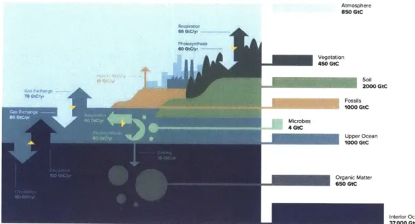
Figure 1-1 presents an illustration of the carbon cycle. Both its global nature and the interweaving of biotic and abiotic components are evident. While the carbon cycle is a consummate complex system, and therefore will be grossly oversimplified by any such representation, a few key features of interest for our present purposes can be gleaned. 1) The ocean - particularly the deep ocean - is the dominant reservoir of surficial carbon (i.e. carbon in the surface Earth) [Sarmiento, 2013, Williams and Follows, 2011, Schlesinger, 1991]. Even the organic carbon content of the deep ocean, a small fraction of the total carbon in the deep ocean, is comparable to the atmosphere's total carbon content. The total oceanic carbon content is an order of magnitude larger than that of all other reservoirs combined. This underscores, at least on long timescales, the dominance of processes controlling the carbon transformations within the deep ocean and the exchanges of carbon between the deep ocean and other components of the system. 2) The surface ocean mediates the exchange of carbon between the deep ocean and the atmosphere (and thus the terrestrial components of the carbon cycle as well) [Sarmiento, 2013, Williams and Follows, 2011, Schlesinger, 1991]. One can also see that the net flux between the surface ocean and the atmosphere is small relative to the gross fluxes from either to the other, such that the surface ocean and atmosphere are nearly in equilibrium in terms of carbon storage. This further underscores the central importance of the vertical distribution of carbon in the ocean1. 3) Despite comprising a relatively negligible reservoir of carbon, marine biota drive a carbon flux from the surface to the deep ocean on the order of the flux of carbon into the atmosphere due to fossil fuel burning and cement production [Sarmiento, 2013, Williams and Follows, 2011, Schlesinger, 1991]. (Note that this flux is largely balanced by a net upwards exchange of carbon from the deep ocean into the surface ocean, which results from higher carbon concentrations in deep ocean water.) This underscores the importance of this downward flux of carbon due to marine biota in controlling the vertical distribution of carbon in the ocean. Altogether, then, this illustration suggests that this flux has an appreciable influence on the global carbon cycle.

These observations are encapsulated in a further idealized depiction of the carbon cycle in Figure 1-2. One may neglect terrestrial fluxes and stores, and consider the partitioning of carbon between the atmosphere, surface ocean, and deep ocean. Carbon is exchanged across

'While one might describe this more coarsely, but in better keeping with Figure 1-1, as the partitioning of carbon between the surface and deep ocean, the above description is less preferable because the distinction between 'surface' and 'deep' ocean is a useful but unavoidably inexact construction.

Atmosphere 850 GtC Vegetation 450 GtC soil 2000 GtC Fossils 1000 GtC Microbes 4 GtC

-

Figure 1-1: Illustration of the global carbon cycle.

the ocean-atmosphere interface and the surface ocean equilibrates with the atmosphere. The deep and surface ocean exchange carbon via ocean circulation and diffusion, and the there is also a biological 'export' of carbon from the surface ocean into the deep [Cael et al., 2017, Ito and Follows, 2005, Williams and Follows, 2011, Goodwin et al., 2008]. The deep ocean carbon concentration is then the sum of a contribution from subducted surface waters and a biologically mediated accumulation. The biologically mediated pool is here assumed to represent the accumulation due to the same marine-biota-driven flux discussed above. Thus in this simple depiction, this flux maintains a vertical gradient of carbon in the ocean, thereby reducing the carbon content of all other reservoirs [Volk and Hoffert, 19851. But what is this flux?

Though somewhat of a misnomer, for historical reasons the collection of processes that comprise this flux are referred to as the biological (carbon) pump. Volk and Hoffert [Volk and Hoffert, 1985] initially defined two2 _{biotic ocean carbon pumps, i.e. processes that deplete} the ocean surface of carbon relative to deep waters: biological fluxes of i) organic carbon and ii) CaCO3. Far more carbon is fluxed in organic form, though individual estimates of these pumps' magnitudes vary and also depend greatly on the definition of the interface

2

Volk and Hoffert [Volk and Hoffert, 1985] also defined a third, abiotic solubility pump resulting from increased CO_{2 solubility in cold downwelling water, that accounts for about a third of the difference in} surface vs. deep dissolved inorganic carbon.

XCo

2

F

4,

V

Atmosphere

Surface Ocean

Csurf

=

Csat

Deep Ocean

Figure 1-2: Simplified illustration of the carbon cycle, taken from Figure S2 of [Cael et al., 2017].

between the surface and deep ocean [Siegel et al., 2014, Palevsky and Doney, 2018, Kwon et al., 20091. The flux of organic carbon can in turn be decomposed further into contributing sub-processes, e.g. sinking of various classes of particles [Fowler and Knauer, 1986], vertical migration of zooplankton [Turner, 2015], or subduction of dissolved or suspended material [Omand et al., 2015]. Of these, particles are the largest vector of carbon transport to the deep sea overall [Buesseler and Boyd, 2009], though other processes can dominate in some situations. Whatever the level of resolution considered, in aggregate these biotic processes are the constituents of the biological pump, that flux which in large part maintains the ocean's vertical gradient in carbon concentration.

The biological pump is of interest not only for its impact on this vertical gradient and therefore atmospheric carbon, but also as a fundamental feature of marine ecology and elemental cycling. The entry of carbon, energy, and other elements into the marine biosphere is concentrated in the thin lens that is the sunlit surface ocean, whereas the consumption of this mass and energy occurs throughout the entire ocean [Schlesinger, 1991, Sarmiento, 2013, Williams and Follows, 2011]. The downward flux therefore transports organic matter from source to sink, connects the global ocean microbiome, and supplies the metabolism of the largest habitat on Earth: the deep sea. The workings of the biological pump are therefore of great interest from several angles.

It comes then as no surprise that the biological pump is the subject of a substantial literature. A number of modeling studies explore the structure, function, and sensitivity of the biological pump; these studies also confirm its global significance, corroborating that the ocean exerts a dominant control on atmospheric carbon and that the biological pump is an essential feature of the marine carbon cycle and microbiome [Kwon et al., 2009, Ito and Follows, 2005, Sarmiento and Toggweiler, 1984, Siegenthaler and Wenk, 1984, Marinov et al., 2008, Cox et al., 2000, Quer6 and Others, 2007]. The biological pump has also been of sustained observational interest which continues today (e.g. the EXPORTS field campaign [Siegel and Others, 2016]), using as broad an array of measurement techniques and experimental designs as any problem in oceanography.

From these efforts a general portrait of the biological pump can be deduced. In the surface ocean, phytoplankton fix dissolved carbon into organic compounds via photosyn-thesis. Globally, this occurs at a rate of roughly ~60 GtC/yr [Buitenhuis et al., 2013] after subtracting autotrophic respiration, though the rate of net carbon fixation (termed

net primary production, NPP) both fluctuates and varies greatly over time and space [Cael et al., 2018]. Much of this carbon is respired and thus returned to its dissolved form by various heterotrophic microorganisms in the surface ocean such as bacteria and zooplank-ton, but a fraction leaves, or is 'exported' from, the surface ocean. By 'a fraction' it is meant something roughly an order of magnitude less than total NPP - the most commonly quoted range of estimates at present is 5-12 GtC/yr [Siegel et al., 2014], though this range depends on the surface through which the flux is defined and one can readily find estimates <5 or >12 GtC/yr - while the local fraction of NPP exported (often termed the 'export efficiency') varies substantially on local spatiotemporal scales, anywhere from close to 0 to close to 1 [Cael and Follows, 2016]. By 'exported' it is meant fluxed downward from the surface ocean either in the form of 'marine snow' aggregates of detrital material, as liv-ing or minimally degraded whole phytoplankton, as zooplankton fecal pellets, as physically subducted suspended material, as vertically migrating organisms, or as some other distinct pathway. By 'the surface ocean' it is often meant either the euphotic layer - the portion of the ocean receiving enough sunlit to sustain net photosynthetic activity, the mixed layer - the upper ocean boundary layer that is considered vertically homogenized by turbulence, or a fixed depth, commonly 100m; in practice all of the above are operationally defined to some extent [Palevsky and Doney, 2018]. The carbon exported is primarily particulate and organic (particulate organic carbon, POC), and is accompanied by particulate organic nitrogen, phosphorous, and various other materials such as biogenic silica or calcium car-bonate [Schneider et al., 2003, Klaas and Archer, 2002]. The efficiency of the biological pump is closely related to the fraction of nutrients that are used to fuel NPP (and therefore associated with carbon) before being subducted; the more nutrients are 'preformed' (i.e. are subducted into the ocean interior without having fueled primary production in the surface ocean), the less efficient the biological pump [Ito and Follows, 2005]. The relatively larger nutrient utilization in high latitudes results in increased carbon storage and higher export efficiency, suggesting a disproportionate global role for high latitude oceans relative to their small areal extent [Sarmiento and Toggweiler, 1984]. Below the surface ocean, the vertical flux attenuates with depth, as microorganisms both attached to particles and within the wa-ter column consume, degrade, break apart, and in general solubilize or remineralize sinking particulate material. Depending on the depth at which sinking material is returned to the water column, it can remain sequestered from the surface ocean from months to millennia

[Kwon et al., 2009, Siegel and Others, 2016]; the climatic impact of the biological pump is thus very sensitive to the depths at which sinking material is remineralized. Various interdependencies between the atmospheric carbon concentration and the biological pump suggest in the net a complex climate-biosphere feedback. Many of these essential features are captured in Figure 1-3.

One can rightly say that the above portrait is rather uncertain and qualitative. Indeed, much of the fundamentals of the biological pump remain poorly understood; neither its global magnitude, nor its structure or variability over space and time, nor its attenuation with depth are well-characterized. Even less established are the relative importance of different pathways, how the dominant mechanisms controlling these pathways work, or how these are likely to change/have changed in the future/past. As an example: what governs how much POC makes it into the bathypelagic? Is this 'refractory' POC that is either not palatable or only very slowly degraded by microorganisms [Jiao and Others, 2010]? Or is this POC labile but physically protected from degradation by associated 'ballast' minerals [Armstrong et al., 2001]? Or does POC degradation simply proceed more slowly with increasing depth due to the much lower temperatures experienced by microbes in the deep sea [L6pez-Urrutia et al., 2006]? Or is this POC transported by very fast-sinking particles that give microbes little time to act [Fowler and Knauer, 1986]? Likely all of these processes can and do influence how much POC is fluxed into the bathypelagic, more or less at different places and times, but in what combination, when and where, and what determines this?

The biological pump's persistent mysteriousness can largely be ascribed to two factors: its complexity, and the difficulty of its measurement. To quote from Section 4.2:

In the ocean, particle flux is nothing if not complex and heterogeneous. Total fluxes comprise myriad sinking particles which are themselves the complex result of myriad biological, chemical, and physical factors [de la Rocha and Passow, 2007]. These particles' physical properties vary widely, from their size and shape to their density and porosity [Kajihara, 1971, Alldredge and Gotschalk, 1988]. Individual particles themselves are comprised of a complex suite of organic and inorganic materials, which may represent a continuum ranging from highly labile to utterly refractory [Hedges et al., 2001, Dittmar, 2008, Jiao and Others, 2010]. Beyond this, the remineralization of particulate material is plausibly related to properties of the ambient fluid like temperature or oxygen concentration [Mooy

Pkco Phyto _zoo Phyto 1 2 3 S2 3 I'. .5% .5

EZ

17

Figure 1-3: Illustration of the pathways of the biological pump, taken from Figure 4 of

[Siegel and Others, 2016].

26

.a

0

v

et al., 2002], may occur via consumption by different bacteria using different metabolic/chemical pathways even within a single particle [Bianchi et al., 2018], may occur at different rates due to the physical microstructure of the particle [Rothman and Forney, 2007], and may in turn alter the shape and other physical properties of the particle [Mayor et al., 2014]. Settling velocity is also related to the density of the ambient fluid, which of course changes with depth due to stratification [Maclntyre et al., 1995]. Individual particles may also interact with each other through myriad aggregation and disaggregation events [Burd and Jackson, 2009, Jackson and Burd, 1998, Alldredge et al., 1990], may be consumed or otherwise altered by free-swimming zooplankton [Steinberg et al., 2008, Kiorboe, 2000, Steinberg, 1995], etc.

Beyond this, neither zooplankton migration nor the submesoscale turbulence responsible for most physical subduction are any simpler - both are active areas of research and their general impacts are beyond robust quantification at present. One can readily see the diffi-culties in accounting for all of these processes rigorously, even in a highly controlled setting. Further complicating this is that POC flux is no simple thing to measure, often involving extended deployment of sediment traps that collect sinking material or inferred indirectly from chemical radiotracers that estimate POC flux on different effective timescales than the measurements of related processes and are subject to similarly large uncertainties as sediment traps [Buesseler, 1991, Buesseler and Others, 2000, Stanely et al., 2004, Buesseler and Others, 2007]. In other words, POC flux is a dynamic result of a large number of interactions between different organisms and with their physiochemical environment, which varies with space and time even on small scales and can only be measured somewhat accu-rately, usually by methods that are expensive and intensive. Where these measurements are made, the number of potentially important covariates is substantial, beyond the ability of most observational campaigns to capture - and the measurement of many of these covariates themselves present significant challenges. Thus the biological pump is not an easy thing to measure or to model.

Even while a complete description of the biological pump might require a great deal more data and detailed understanding of all of these factors' interdependencies, insight is the product of simplicity, and for many applications an approximate quantitative description of the biological pump and what controls its variations is sufficient. Certain relationships

between POC flux and other phenomena have been proposed that make mechanistic sense and are empirically supported; in cases where sufficient data are available, simple and general relationships can be deduced that provide valuable intuition about the biological pump (though these may not always provide satisfactory predictive power). These relationships tend to be with more 'basic' variables - e.g. the temperature of the surrounding fluid, rather than e.g. the mean fractal dimension of marine snow aggregates. A formative paper by Eppley and Peterson [Eppley and Peterson, 1979], building on the work of Dugdale and Goering [Dugdale and Goering, 1967], argued from a steady-state perspective that POC export should be approximated by new production (NPP fueled by nutrients externally injected into the euphotic layer, primarily by the upwelling of nutrient-rich deep waters), and that new production is an increasingly large fraction of total production as total production increases - therefore that export efficiency increases with productivity. Suess [Suess, 1980] looked further at the relationship between POC flux and NPP to include depth, and found an approximately inverse relationship between flux and depth. Laws et al [Laws et al., 2000b], examining a detailed numerical model of the planktonic ecosystem, concluded that export efficiency should also be determined by mixed layer temperature; a small self-consistent set of observations corroborated this interpretation, with both suggesting a negative linear relationship between export efficiency and temperature. Relationships with other variables or processes, e.g. different metrics of community structure [Guidi et al., 2009], have been proposed - these relationships are however more challenging to assess, quantify, and measure than these basic oceanographic variables of temperature, depth, and productivity.

Subsequent literature has built upon these initially posited relationships, incorporating over time the additional constraints of many more observations, and exploring the validity of different, sometimes contradictory, models to relate POC flux to these other variables. The simple correspondences between these and POC flux are not clearly supported by these expanded datasets, which instead reflect the highly variable nature of POC flux, e.g. [Maiti et al., 2013, Dunne et al., 2005, Henson et al., 2011, Bisson et al., 2018]. Thus it is necessary to revisit these relationships in this context and to develop new models that capture the relationship between POC flux and these other variables while also acknowledging and being consistent with this variability. Improving our understanding of how these basic variables relate to POC flux can help provide a general quantitative characterization of the biological pump despite its complexity and variability. Export efficiency may not be a simple linear

function of temperature, but the fundamental insight underlying Laws et al. [Laws et al., 2000b] that temperature should influence export efficiency is no less plausible - perhaps temperature is one of many influences, and the mechanistic and quantitative nature of this influence can still be extracted. Even if individual measurements of NPP and POC flux seem to suggest differing or very weak relationships, the mechanistic link between the two is fundamental - all of the sinking material that comprises POC must previously be fixed via NPP - so it should be possible to identify some quantitative relationship between the two. And there is plenty of room for progress in understanding quantitatively and mechanistically the depth-attenuation of POC flux that determines the fate of this exported material. As the scientific community invests ever-greater resources into the study of the biological pump, there is a need to compile and make sense of the data that are out there.

To summarize: the biological pump is an integral component of the carbon cycle, marine ecology, and climate. While the biological pump has been the subject of much investigation, because of its complexity and variability, along with the extremely difficult nature of its measurement, in its characterization there is much room for improvement. The sinking flux of particulate organic carbon is thought to be the dominant vector of transport for the biological pump. Key relationships between this flux and temperature, productivity, or depth have been identified; specifying this flux in terms of these variables yields a necessarily oversimplistic yet still valuable description. These relationships are less clear in the light of additional data and analyses thereof, suggesting a need to revisit these relationships and to find ways of describing them that are consistent with the variability exhibited by these data. By pairing compilations of extant data with novel mathematical models, this thesis attempts to address this need.

The modeling approach taken here is to incorporate variability and/or heterogeneity in the biological pump by describing certain quantities as random variables sampled from prob-ability distributions - what we will refer to as a distributional approach. Rather than con-sidering export efficiency as a function of temperature, i.e. ef = ef(T), we consider export

efficiency as a random variable sampled from a probability distribution that is temperature-dependent, i.e. ef ~ Pef = Pef(T). This is not to suggest that export efficiency is actually a random process, but rather that a number of factors, of which temperature is one, influence export efficiency, and in the absence of information about these other processes, we may for simplicity assume that they influence export efficiency in a way that appears to us as

dom. Rather than considering POC flux as a function of NPP, i.e. F = F(NPP), we consider POC flux as a random variable sampled from a probability distribution that is a function of the probability distribution that NPP is sampled from, i.e. F ~ PF = PF(PNPP). Rather than considering a single settling velocity w for sinking particles, we consider particulate material to sink heterogeneously at varying speeds, collectively described by a distribution P,. Though only minimally more sophisticated than standard statistical models for these relationships, this type of distributional approach allows us to make appreciable progress in capturing the observed relationships, without idealizing out the variability that evinces the system's complexity. We apply this distributional perspective to each of the relationships discussed above in turn.

Chapter 2 addresses the relationship between export efficiency and temperature. A simple mechanistic-distributional model for the relationship between export efficiency and temperature is derived from considering the dynamics of a phytoplankton population in the mixed layer. The underlying mechanism is the differential temperature sensitivity of totrophic and heterotrophic processes; as temperatures increase, the maximum rate of au-totrophy increases, but the typical rate of heterotrophic processes increases even more so, as reflected in growth-temperature relationships of phytoplankton and zooplankton. The model predicts that the distribution of export efficiency measurements is scaled, or 'squeezed,' by the temperature of the mixed layer; the model extracts the temperature dependency of a collection of observations >2 orders of magnitude larger than the original dataset considered by Laws et al. [Laws et al., 2000b]. The model is then applied to global sea surface temper-ature records to estimate a decline in global average export efficiency of 1-2% over the past three decades due to this metabolic mechanism. Finally, incorporation of this temperature sensitivity into a simple box model framework suggests that this mechanism accounts for a ~7 ppm K- 1 decrease in atmospheric

pCO

Chapter 3 addresses the relationship between export and net primary production. As described above, NPP and export are inextricable by mass conservation, but the quantitative relationship between the two is elusive. We hypothesize that a qualitative relationship should emerge between collections of the two measurements, because they are measured on different effective spatiotemporal scales. We therefore describe the basis of a theory for interpreting measurements of the two fluxes in terms of their probability distributions. We take as

a null model that both should be lognormally distributed on large scales, and show that compilations of measurements of each are consistent with this hypothesis. The compilation of NPP measurements is extensive enough to subregion by biome, basin, depth, or season; these subsets are also well described by lognormals, whose log-moments sort predictably. Informed by this robust lognormality we infer a statistical scaling relationship between the two fluxes. Two independent estimates of the relationship between the distributions' log-moments agree, illustrating the utility of a distributional approach to biogeochemical fluxes and suggesting that POC flux is predictable from NPP on large scales.

Chapter 4 addresses the relationship between POC flux and depth. Several idealized models for this relationship are derived mechanistically, and the mechanistic differences be-tween these models are highlighted. A large quantitative difference bebe-tween these models is then demonstrated; from the same POC flux measurements, these models estimate widely different magnitudes of export (i.e. POC flux normalized to a reference depth such as the euphotic or mixed layer depth) and remineralization lengthscales at shallow depths. In contrast, it is shown that these models are quantitatively indistinguishable from available measurements, given the variability and uncertainty of POC flux measurements and the flex-ibility and similarity of these models over the depths at which most POC flux measurements are made, indicating the need to leverage additional measurements to produce multiple con-straints. Next we propose a mechanistic, distributional model for the depth-attenuation of marine particle flux, that takes into account measurements of both the flux profile and the settling velocity distribution of particulate matter. Settling velocity distribution mea-surements are best captured by a reciprocal distribution. This distribution then implies a two-parameter model for the flux-depth relationship if it is assumed that the bulk flux profile is the superposition individual particles' fluxes and controlled by the initial variation in settling velocity. This model also fits measured flux profiles equivalently to or better than standard models. Though necessarily oversimplistic, it is therefore unique in captur-ing observations of both flux vs. depth and of the settlcaptur-ing velocity distribution, and thus constitutes a particle flux parameterization that is more consistent with and constrained by empirical knowledge. Furthermore, the emergence of the reciprocal distribution underlying the model is predictable as a result of the large number of processes that produce sinking particulate material. The model also generates multiple hypotheses that are testable in situ. Lastly, Chapter 5 summarizes the main findings of the preceding chapters and discusses

several possible avenues of future inquiry. These avenues include both theoretical - e.g. ap-plying the model developed in Chapter 2 to glacial-interglacial atmospheric pCO2 changes

- and observational - _{e.g. testing the model developed in Chapter 4 in situ} - research, ranging from specific and targeted to broad and general. In the end, a great deal more work is required to come to a rigorous understanding of the biological pump and its relationship to other oceanic phenomena such as those examined herein.

Chapter 2

Temperature and export efficiency

The work in this chapter is based upon the following publications:

Cael, B. B., and M. J. Follows. 2016. On the temperature dependence of oceanic export efficiency. Geophysical Research Letters. [Cael and Follows, 2016]

Cael, B. B., K. Bisson, and M. J. Follows. 2017. How have recent temperature changes affected the efficiency of ocean biological carbon export? Limnology and Oceanography: Letters. [Cael et al., 2017]

2.1

On the temperature dependence of oceanic export

effi-ciency

2.1.1 Overview

Quantifying the fraction of primary production exported from the euphotic layer (termed the export efficiency ef) is a complicated matter. Studies have suggested empirical rela-tionships with temperature which offer attractive potential for parameterization. Here we develop what is arguably the simplest mechanistic model relating the two, using established thermodynamic dependencies for primary production and respiration. It results in a single-parameter curve that constrains the envelope of possible efficiencies, capturing the upper bounds of several ef-T data sets. The approach provides a useful theoretical constraint on this relationship and extracts the variability in ef due to temperature but does not ideal-ize out the remaining variability which evinces the substantial complexity of the system in question.

2.1.2 Introduction

The export of organic carbon out of the upper ocean is an important component of the climate system, driving the "biological pump" which reduces the partial pressure of atmo-spheric carbon dioxide and fuels the ecosystems of the deep ocean and benthos [Archer et al., 2000]. The efficiency with which limiting resources (usually nutrients) are exported, relative to local recycling, is often termed the ef ratio, here defined as the ratio of the sinking flux of particulate organic carbon across a defined depth horizon and the integrated primary production Pp above that horizon, e.g., [Laws et al., 2000b]. Eppley and Peterson [Eppley and Peterson, 1979] identified a simple, empirical relationship between ef and integrated primary production, but it has been difficult to establish a clear theoretical basis for the controls on ef due to the myriad physical and biological processes at play [de la Rocha and Passow, 2007].

Laws et al. [Laws et al., 2000b] examined a relatively detailed numerical model of the planktonic ecosystem, which suggested that ef is shaped by PP and mixed layer temperature T. A compilation of self-consistent observations of export efficiency ef along with local physical and biogeochemical factors, from the Joint Global Ocean Flux Study (JGOFS) Process Study data, supported this interpretation. Both model and data suggested an approximately linear, negative correlation between ef and mixed layer temperature, T, and that the temperature dependence of the ecosystem processes which shape export production provide a dominant control on ef. Indeed, the temperature variation explained far more of the variance in ef than P, in that data set. A series of subsequent studies [Laws et al., 2000a, Henson et al., 2011, Dunne et al., 2005, Maiti et al., 20131 have explored the validity and possible forms of temperature-ef relationships, and there has been a significant increase in the empirical data constraints over the past 15 years. The simple correspondence between ef and T of Laws et al. [Laws et al., 2000b] is not clearly supported with a much expanded data set. Consequently, recent models and interpretations of these data sets have not lead to a consistent, simple relationship between ef and T.

However, Laws et al. [Laws et al., 2000a] revisited the ef-T relationship from an em-pirical perspective, showing that the upper bound of ef declines as temperature increases. Here we consider this upper bound from a mechanistic perspective. At the heart of the temperature dependence in the Laws et al. [Laws et al., 2000b] model is the differential

temperature sensitivity of phototrophic and heterotrophic metabolism [L6pez-Urrutia et al.,

2006, Huntley and Lopez, 1992, Eppley, 19721 (clearly characterized by Rose and Caron

[Rose and Caron, 20071). We develop a highly idealized framework which reflects this key element. We argue that while finding a simple relationship between ef and T will be con-founded by many other factors in real systems, there is a predictable mechanistic relationship between the maximum export ratio, efmax and T which reflects situations where all other limitations and constraints (e.g., nutrients) are relaxed, analogous to the interpretation of the Eppley Curve [Eppley, 1972] (see Figure 2-1). There the simple parameterization relates to the upper bound of growth rate: in any given circumstance other factors such as nutri-ent limitation might restrict growth and so only the maximum of the observed data points represents the effect of temperature clearly.

Hence, we seek to characterize an envelope bounding export efficiency based on thermo-dynamic constraints. To do so, we will write the simplest model which captures the essential dynamics (Section 2.1.3). Starting with an ordinary differential equation describing the time rate of change of autotrophic biomass, we derive a predicted curve for maximum export effi-ciency as a function of temperature. In Section 2.1.4 we show that this simple, mechanistic model captures the trends in a compilation of empirical data with global coverage [Laws et al., 2000b, Dunne et al., 2005, Henson et al., 2011, Buesseler and Boyd, 2009 and discuss the value and limitations of the framework.

2.1.3 Temperature vs. export efficiency: Model and Data

We first write a simple ordinary differential equation for the phytoplankton biomass density

(p) in the upper ocean (the mixed layer, or euphotic zone, or above the thermocline):

5 = P - Ap - A'p - wp (2.1)

where p is a linear growth rate, / represents loss due to grazing, and A' represents losses from other processes including, e.g., viral lysis, senescence, and detrainment. w represents the rate of export as sinking particles; all coefficients have dimensions of inverse time. Assuming steady state and dividing through by pp, Eq. (2.1) becomes

0 = - A A'+ (2.2)

Figure 2-1: Temperature sensitivity for phytoplankton and copepod growth rates, adapted from (a) Eppley [Eppley, 1972] and (b) Huntley and Lopez [Huntley and Lopez, 1992]. The temperature scaling prefactor is larger for the copepods, the key thermodynamic relation that drives this model. Another key difference is that copepod growth clusters along, while phytoplankton growth lies under, their respective curves; copepod growth appears to deviate significantly from this curve near T = 24 C. These predictions from the above pictured original data sets have been additionally tested and verified in, e.g., Rose and Caron [Rose and Caron, 2007]. Note the x axes of each subplot cover different limits. The prefactor is

the value which multiplies temperature in the expressions p oc eO.063T e .A 1c

Eppley Curve: prefactor = .0633

12+ ,:-' 10 6+ CD 4 4 + --2 $ + + + + 5 10 is 20 25 30 35 40 45

1.5 - Huntley & Lopez Curve: prefactor = .11

0.5 + + +

0

0 5 10 15 20 25 30

Temperature [deg C]