HAL Id: hal-01387031
https://hal.archives-ouvertes.fr/hal-01387031
Submitted on 22 Dec 2016
HAL is a multi-disciplinary open access
archive for the deposit and dissemination of
sci-entific research documents, whether they are
pub-lished or not. The documents may come from
teaching and research institutions in France or
abroad, or from public or private research centers.
L’archive ouverte pluridisciplinaire HAL, est
destinée au dépôt et à la diffusion de documents
scientifiques de niveau recherche, publiés ou non,
émanant des établissements d’enseignement et de
recherche français ou étrangers, des laboratoires
publics ou privés.
Maroua Maalej, Vitor Paisante, Ramos Pedro, Laure Gonnord, Fernando
Pereira
To cite this version:
Maroua Maalej, Vitor Paisante, Ramos Pedro, Laure Gonnord, Fernando Pereira. Pointer
Disam-biguation via Strict Inequalities. Code Generation and Optimisation , Feb 2017, Austin, United
States. pp.134-147. �hal-01387031�
C o nsist ent *Complete*W ellDo cu m en ted *E asy to Re us e * * Ev alu ate d * C G O *Ar tifact* AE C
Pointer Disambiguation via Strict Inequalities
Maroua Maalej
Univ. Lyon, France & LIP (UMR CNRS/ENS Lyon/UCB Lyon1/INRIA) Maroua.Maalej@ens-lyon.fr
Vitor Paisante
UFMG, Brazil paisante@dcc.ufmg.brPedro Ramos
UFMG, Brazil pedroramos@dcc.ufmg.brLaure Gonnord
Univ. Lyon1, France & LIP(UMR CNRS/ENS Lyon/ UCB Lyon1/INRIA) Laure.Gonnord@ens-lyon.fr
Fernando Magno Quint˜ao Pereira
UFMG, Brazilfernando@dcc.ufmg.br
Abstract
The design and implementation of static analyses that dis-ambiguate pointers has been a focus of research since the early days of compiler construction. One of the challenges that arise in this context is the analysis of languages that support pointer arithmetics, such as C, C++ and assem-bly dialects. This paper contributes to solve this challenge. We start from an obvious, yet unexplored, observation: if a pointer is strictly less than another, they cannot alias. Moti-vated by this remark, we use abstract interpretation to build strict less-than relations between pointers. We construct a program representation that bestows the Static Single Infor-mation (SSI) property onto our dataflow analysis. SSI gives us a sparse algorithm, whose correctness is easy to ensure. We have implemented our static analysis in LLVM. It runs in time linear on the number of program variables, and, de-pending on the benchmark, it can be as much as six times more precise than the pointer disambiguation techniques al-ready in place in that compiler.
Keywords Alias analysis, range analysis, speed, precision
1.
Introduction
Pointer disambiguation consists in determining if two point-ers, p1 and p2, can refer to the same memory location.
If overlapping happens, then p1 and p2 are said to alias.
Pointer disambiguation has been focus of much research [3, 15, 17, 34], since the debut of the first alias analysis ap-proaches [6, 33]. Today, state-of-the-art algorithms have ac-ceptable speed [15, 28], good precision [40] or meet each other halfway [16, 36]. However, understanding the rela-tionships between memory references in programming lan-guages that support pointer arithmetics remains challenging.
Pointer arithmetics come from the ability to associate pointers with offsets. Much of the work on automatic paral-lelization consists in the design of techniques to distinguish offsets from the same base pointer. Michael Wolfe [42, Ch.7] and Aho et al. [1, Ch.11] have entire chapters devoted to this issue. State-of-the-art approaches perform such distinc-tion by solving diophantine equadistinc-tions, be it via the greatest common divisor test, be it via integer linear programming, as Rugina and Rinard do [31]. Other techniques try to associate intervals, numeric or symbolic, with pointers [4, 26, 27, 44], presenting different ways to build Balakrishnan and Reps’ notion of value sets. And yet, as expressive and powerful as such approaches are, they fail to disambiguate locations that are obviously different, as v[i] and v[j], in the loop:
for(i = 0, j = N; i < j; i++, j−−) v[i] = v[j]; In this paper, we present a simple and efficient solution to this shortcoming. We say that v[i] and v[j] are obviously different locations because i < j. There are techniques to compute less-than relations between integer variables in pro-grams [7, 20, 21, 23]. Nevertheless, so far, they have not been used to disambiguate pointer locations. The insight that such techniques are effective and useful to such purpose is the key contribution of this paper. However, we go beyond: we rely on recent advances on the construction of sparse dataflow analyses [38] to design an efficient way to solve less-than in-equalities. The sparse implementation lets us view this prob-lem as an instance of the abstract interpretation framework; hence, we get correctness for free. The end result of our tool is a less-than analysis that can be augmented to handle dif-ferent program representations, and that can increase in non-trivial ways the ability of compilers to distinguish pointers.
To demonstrate this last statement, we have implemented our static analysis in the LLVM compiler [19]. We show
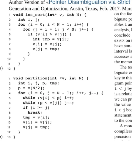
void ins_sort(int* v, int N) { int i, j; for (i = 0; i < N − 1; i++) { for (j = i + 1; j < N; j++) { if (v[i] > v[j]) { int tmp = v[i]; v[i] = v[j]; v[j] = tmp; } } } }
void partition(int *v, int N) { int i, j, p, tmp;
p = v[N/2];
for (i = 0, j = N - 1;; i++, j--) { while (v[i] < p) i++;
while (p < v[j]) j--; if (i >= j) break; tmp = v[i]; v[i] = v[j]; v[j] = tmp; } } 1 2 3 4 5 6 7 8 9 10 11 12 1 2 3 4 5 6 7 8 9 10 11 12 13 (a) (b)
Figure 1. Two snippets of C code that challenge typical pointer disambiguation approaches.
empirically that industrial-quality alias analyses still leave unresolved pointers which our simple technique can dis-ambiguate. As an example, we distinguish 11,881 pairs of pointers in SPEC’s lbm, whereas LLVM’s analyses dis-tinguish 1,888. Furthermore, by combining our approach with basic heuristics, we obtain even more impressive re-sults. For instance, our less-than check increases the success rate of LLVM’s basic disambiguation heuristic from 48.12% (1,705,559 queries) to 64.19% (2,274,936) in SPEC’s gobmk.
2.
Overview
To motivate the need for a new points-to analysis we show its application on the programs seen in Figure 1. The fig-ure displays the C implementation of two sorting routines that make heavy use of pointers. In both cases, we know that memory positions v[i] and v[j] can never alias within the same loop iteration. However, traditional points-to anal-yses cannot prove this fact. Typical implementations of these analyses, built on top of the work of Andersen [3] or Steens-gaard [34], can distinguish pointers that dereference differ-ent memory blocks; however, they do not say much about references ranging on the same array.
There are points-to analyses designed specifically to deal with pointer arithmetics [2, 4, 24, 27, 31, 32, 37, 39, 41]. Still, none of them works satisfactorily for the two exam-ples seen in Figure 1. The reason for this ineffectiveness lays
on the fact that these analyses use range intervals to disam-biguate pointers. In our examples, the ranges of integer vari-ables i and j overlap. Consequently, any conservative range analysis, `a la Cousot [10], once applied on Figure 1 (a), will conclude that i exists on the interval [0, N − 2], and that j exists on the interval [1, N − 1]. Because these two intervals have non-empty intersection, points-to analyses based on the interval lattice will not be able to disambiguate the memory accesses at lines 6-8 of Figure 1 (a). The same holds true for the memory accesses in Figure 1 (b).
The technique that we introduce in this paper can disam-biguate every use of v[i] and v[j] in both examples. The key to this success is the observation that i < j at every pro-gram point where we have an access to v. We conclude that i < j by means of a “less-than check”. A less-than check is a relationship between two variables that is true whenever we can prove – statically – that one holds a value lesser than the value stored in the other. In Figure 1 (a), we know that i < j because of the way that j is initialized, within the for statement at line 4. In Figure 1 (b), we know that i < j due to the conditional check at line 7.
A more precise alias analysis brings many advantages to compilers. One of such benefits is optimizations: the extra precision gives compilers information to carry out more ex-tensive transformations in programs. Notice that the pointer analysis that we propose in this paper provides weaker guar-antees than more traditional approaches. Continuing with our example, the pointers v[i] and v[j] in Figure 1 (a & b) do, indeed, alias across the entire loop nest, albeit not at the same time. As we shall discuss in Section 3.5, if we say that two pointers do not alias, then they will never alias at any program point where they are simultaneously alive. This property is strong enough to support most of the classic com-piler optimizations: constant propagation, value numbering, subexpression elimination, scheduling, etc. However, our technique cannot be used with optimizations that modify the iteration space of programs, such as loop fission and fusion.
3.
The Less-Than Check
This section introduces a dataflow analysis whose goal is to construct a “less-than” set for each variable x (pointer or numeric, as we will discuss in Section 3.6). We denote such an object by LT(x). As we prove in Section 3.5, the important invariant that this static analysis guarantees is that if x0 ∈ LT(x), then x0 < x at every program point
where both variables are alive. Our ultimate goal is to use this invariant to disambiguate pointers, as we explain in Section 3.6.
3.1 The Core Language
We use a core language to formalize the developments that we present in this paper. Figure 2 shows the syntax of this language. Our core language contains only those instruc-tions that are essential to describe our static analysis. The
Integer constants ::= {c1, c2, . . .} Variables ::= {x1, x2, . . .} Program (P) ::= {`1: I1; . . . , `n: In; } Instructions (I) ::= – Addition | x0= x1+ x2 – φ-function | x0= φ(x1: `1, . . . , xn : `n)
– Comparison | (x1< x2) ? goto `t : goto `f
Figure 2. The syntax of our language. Variables have scalar type, e.g., either integer or pointer.
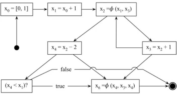
x0 = [0, 1] x1 = x0 + 1 x2 =ɸ (x1, x3)
x3 = x2 + 1 x4 = x2 − 2
(x4 < x1)? true x6 =ɸ (x4, x3, x4) false
Figure 3. Program written in our core language. reader can augment it with other assembly instructions, to make it as expressive as any industrial-strength program rep-resentation. As a testimony to this fact, the implementation that we describe in Section 4 comprises the entire LLVM intermediate representation. Figure 2 describe programs in Static Single Assignment form [12]; therefore, it contains φ-functions. Additionally, it contains arithmetic instructions and conditional branches. These two kinds of instructions feed our static analysis with new information.
EXAMPLE3.1. Figure 3 describes a program in our core language. This is an artificial example, whose semantics is immaterial. Figure 3 illustrates a few key properties of the strict SSA representation: (i) the definition point of a variable dominates all its uses, and (ii) if two variables interfere, one of them is alive at the definition point of the other. Such properties will be useful in Section 3.5.
3.2 Program Representation
We want to implement a sparse dataflow analysis. Sparsity is good for: (i) time and space, as it reduces from cubic to quadratic (on the number of variables) the amount of information that needs to be stored; and (ii) correctness, as it simplifies all the proofs of theorems. A dataflow analysis is said to be sparse if it runs on a program representation that ensures the Static Single Information (SSI) Property [38]. To keep this paper self-contained, we quote Tavares et al.’s notion of single information property:
Instructions (I) ::= – Addition | x0= x1+ x2 – Subtraction | x0= x1− n k hx2= x1i – φ-function | x0= φ(x1: `1, . . . , xn : `n) – Comparison | (x1< x2)? ( `t: hx1t, x2ti `f : hx1f, x2fi
Figure 4. The syntax of our intermediate language. DEFINITION3.2 (Static Single Information Property). A dataflow analysis bears the static single information prop-erty if it always associates a variable with the same abstract state at every program point where that variable is alive.
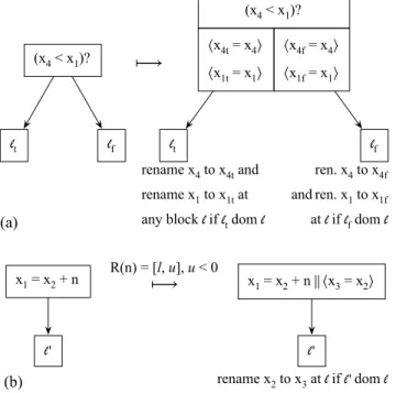
Following Tavares et al. [38], to ensure the SSI property, we split the live range of every variable x at each program point where new information about x can appear. The live range of a variable v is the collection of program points where v is alive. To split the live range of x at a point `, we create a copy x0= x at `, and rename uses of x at every program point dominated by `. We shall write ` dom `0 to indicate that ` dominates `0, meaning that any path from the beginning of the control flow graph to `0must cross `. There are three situations that create new less-than information about a variable x:
1. x is defined. For instance, if x = x0+ 1, then we know that x0< x;
2. x is used in a subtraction, e.g,. x0= x + n, n < 0. In this case, we know that x0< x;
3. x is used in a conditional, e.g., x < x0. In this case, we know that x < x0 at the true branch, and x0 ≤ x at the false branch.
The Support of Range Analysis on Integer Intervals. The SSA representation ensures that a new name is created at each program point where a variable is defined. To meet the other two requirements, we split live ranges at subtractions and after conditionals. Going back to Figure 2, we see that our core language contains only syntax for arithmetic addi-tions. However, we can use range analysis to know that one, or the two, terms of an addition are negative. Range analy-sis [10] is a static dataflow analyanaly-sis that associates each vari-able x to an interval R(x) = [l, u], {l, u} ⊂ N, l ≤ u. The efficient and precise computation of range analysis has been researched extensively in the literature, and we shall not dis-cuss it further. In our experiments, we have used the imple-mentation of Rodrigues et al., which inserts guards in pro-grams to track integer overflows [30]. Given x1= x2+ x3,
where R(x2) = [l2, u2] and R(x3) = [l3, u3], we have a
subtraction if u3< 0 or u2< 0. If both variables have
posi-tive ranges, then we have an addition. Otherwise, we have an unknowninstruction, which shall not generate constraints.
(x4 < x1)? ⟨x4t = x4⟩ ⟨x1t = x1⟩ ⟨x4f = x4⟩ ⟨x1f = x1⟩ (x4 < x1)? lt lf lt lf ⟼ x1 = x2 + n‖⟨x3 = x2⟩ x1 = x2 + n ⟼ l' l' rename x4 to x4t and rename x1 to x1t at any block l if lt dom l
ren. x4 to x4f andren. x1 to x1f at l if lf dom l rename x2 to x3 at l if l' dom l (a) (b) R(n) = [l, u], u < 0
Figure 5. Transformation rules used to convert the syntax in Figure 2 into the syntax in Figure 4.
Our live range splitting strategy leads to the creation of a different program representation. Figure 4 shows the instructions that constitute the new language. Figure 5 shows the two syntactic transformations that convert a program written in the syntax of Figure 2 into a program written in the syntax of Figure 4. We let x0 = x1− n k hx2 = x1i
denote a composition of two statements, x0 = x1− n and
x2= x1. The second instruction splits the live range of x1.
Both statements happen in parallel. Thus, x0 = x1− n k
hx2= x1i does not represent an actual assembly instruction;
it is only used for notational convenience. Similarly, when transforming conditional tests, we let hx1t = x1, x2t = x2i
denote two copies that happen in parallel: x1t = x1, and
x2t = x2. Whenever there is no risk of ambiguity, we
write simply hx1t, x2ti, as in Figure 4. Parallel copies and
φ-functions are removed before code generation, after the analyses that require them have already run. This step is typically called SSA-Elimination phase.
EXAMPLE3.3. Figure 6 shows the result of applying the rules seen in Figure 5 onto the program in Figure 3.
3.3 Constraint Generation
Once we have a suitable program representation, we use the rules in Figure 7 to generate constraints. These constraints determine the less-than set of variables. Constraint genera-tion is O(|V|), where V is the set of variables in the target program. We have four kinds of constraints:
init: Set the less-than set of a variable to empty: LT(x) = ∅.
x0 = • x1 = x0 + 1 x2 =ɸ (x1, x3) x3 = x2 + 1 x4 = x2 − 2 ‖⟨x5 = x2⟩ (x4 < x1)? ⟨x4t = x4⟩ ⟨x1t = x1⟩ ⟨x4f = x4⟩ ⟨x1f = x1⟩ x6 =ɸ (x4, x3, x4t)
Figure 6. Figure 3 transformed by the rules in Figure 5.
x = • 1LT(x) = ∅ x1= x2+ n 2LT(x1) = {x2} ∪ LT(x2) x1= x2− n k hx3= x2i 3 ( LT(x3) = {x1} ∪ LT(x2) LT(x1) = ∅ x = φ(x1, . . . , xn) 4LT(x) = LT(x1) ∩ . . . ∩ LT(xn) (x1< x2)? ( `t: hx1t, x2ti `f : hx1f, x2fi 5 LT(x2t) = {x1t} ∪ LT(x2) ∪ LT(x1t) LT(x1t) = LT(x1) LT(x2f) = LT(x2) LT(x1f) = LT(x1) ∪ LT(x2f)
Figure 7. Constraint generation rules. Numbers labelling each rule are used in the proofs of Section 3.5. If n is constant, then we assume n > 0. If n is a variable, then R(n) = [l, u], l > 0.
union: Set the less-than set of a variable to be the union of another less-than set and a single element: LT(x3) =
{x1} ∪ LT(x2).
inter: Set the less-than set of a variable to be the intersection of multiple less-than sets: LT(x) = LT(x1) ∩ LT(x2).
copy: Sets the less-than set of a variable to be the less-than set of another variable: LT(x) = LT(x0).
EXAMPLE3.4. The rules in Figure 7 produce the follow-ing constraints for the program in Figure 6:LT(x0) = ∅,
LT(x1) = {x0} ∪ LT(x0), LT(x2) = LT(x1) ∩ LT(x3),
LT(x3) = {x2} ∪ LT(x2), LT(x4) = ∅, LT(x5) = {x4} ∪
LT(x2), LT(x1t) = {x4t} ∪ LT(x4t) ∪ LT(x1), LT(x1f) =
LT(x1), LT(x4f) = LT(x1f) ∩ LT(x4), LT(x4t) = LT(x4),
3.4 Constraint Solving
Constraints are solved via a worklist algorithm. We initialize LT(x) to V, for every variable x. During the resolution pro-cess, elements are removed from each LT, until a fixed point is achieved. Theorem 3.7, in Section 3.5, guarantees that this process terminates. Constraint solving is equivalent to find-ing transitive closures; thus, it is O(|V|3). In practice, we
have observed an O(|V|) behavior, as we show in Section 4. EXAMPLE3.5. To solve the constraints in Example 3.4, we initialize everyLT set to {x0, x1, x2, x3, x4, x5, x6, x1f, x1t,
x4f, x4t}, i.e., the set of program variables. The
follow-ing sets are a fixed-point solution of this system:LT(x0) =
LT(x4) = LT(x4t) = LT(x6) = ∅; LT(x1) = LT(x2) =
LT(x4f) = LT(x1f) = {x0}; LT(x3) = {x0, x2}; LT(x5) =
{x0, x4}; and LT(x1t) = {x0, x4t}.
3.5 Properties
There are a number of properties that we can prove about our dataflow analysis. In this section we focus on two core properties: termination and adequacy. Termination ensures that the constraint solving approach of Section 3.4 always reaches a fixed point. Adequacy ensures that our analysis conforms to the semantics of programs. To show termina-tion, we start by proving Lemma 3.6.
LEMMA3.6 (Decreasing). If constraint resolution starts withLT(x) = V for every x, then LT(x) is monotonically decreasing or stationary.
Proof: The proof follows from a case analysis on each con-straint produced in Figure 7, plus induction on the number of elements in LT. Figure 7 reveals that we have only three kinds of constraints:
• LT(x) = ∅: in this case, LT(x) is stationary; • LT(x) = {x0} ∪ LT(x00
): by induction, LT(x00) is de-creasing or stationary, and LT(x) always contains {x0}; • LT(x) = LT(x1) ∩ . . . ∩ LT(xn): we apply induction
on each LT(xi), 1 ≤ i ≤ n.
To prove Theorem 3.7, which states termination, we need to recall PV, the semi-lattice that underlines our less-than analysis. PV = {V, ∩, ⊥ = ∅, > = V, ⊆} is the lattice formed by the partially ordered set of program variables. Ordering is given by subset inclusion ⊆. The meet opera-tor (greatest lower bound) is set intersection ∩. The lowest element in this lattice is the empty set, and the highest is V. THEOREM3.7 (Termination). The constraint resolution pro-cess terminates.
Proof: The proof of this theorem is the conjunction of two facts: (i) Constraint sets are monotonically decreasing; and (ii) they range on a finite lattice. Fact (i) follows from Lemma 3.6. Fact (ii) follows from the definition of PV.
We followed the framework of Tavares et al. [38] to build our intermediate program representation. Thus, we
get correctness for free, as we are splitting live ranges at every program point where new information can appear. Lemma 3.8 formalizes this notion.
LEMMA3.8 (Sparcity). LT(x) is invariant along the live range ofx.
Proof: The proof follows from case analysis on the con-straint generation rules in Figure 7. By matching concon-straints with the syntax that produce them, we find that the abstract state of a variable can only change at its definition point. This property is ensured by the live range splitting strategy that produces the program representation that we use.
We close this section showing adequacy. In a nutshell, we want to show that if our constraint system determines that a variable x belongs into the less-than set of another vari-able x0, then we know that x < x0. This is a static notion: we consider the values of x and x0that exist at the same moment during the execution of a program. Theorem 3.9 formalizes this observation. The proof of that theorem requires the se-mantics of the transformed language, whose syntax appears in Figure 4. However, for the sake of space, we omit this se-mantics. We assume the existence of a small-step transition rule →, which receives an instruction ι, plus a store environ-ment Σ, and produces a new environenviron-ment Σ0. The store maps variables to integer values. Analogously, the constraints of Figure 7 show how instructions change the abstract state LT. We write ι ` LTB LT0 to denote an abstract transition. We let |= model the following relation: if x0 ∈ LT(x), then Σ(x0) < Σ(x). If this relation is true for every element in the domain of Σ, then we write LT |= Σ.
THEOREM3.9 (Adequacy). If LT1 |= Σ1 ∧ ι ` Σ1 →
Σ2∧ ι ` LT1B LT2, thenLT2|= Σ2.
Proof: The proof happens by case analysis on the five instructions in Figure 7. For brevity, we show two cases: First case: ι is x1 = x2 + n. Notice that n > 0 be-cause otherwise our range analysis would have led us to transform that instruction into a subtraction, or would have produced no constraint at all. Henceforth, we shall write “f \ a 7→ b” to denote function update, i.e.: “λx.if x = a then b else f (x)” We have that x1 = x2+ n ` Σ1 → (Σ1 \ x1 7→ Σ1(x2) + n), and x1 = x2 + n ` LT1B (LT1\ x17→ LT1(x2) ∪ {x2}). We look into possible vari-ables x ∈ LT1\ x17→ LT1(x2) ∪ {x2}:
• x = x2: the theorem is true because Σ1(x2) + n > Σ1(x2);
• x ∈ LT(x2): From the hypothesis LT1 |= Σ1, we have that x < x2. We know that x2 < x1; thus, by transitivity, x < x1.
Second case: ι is a φ-function. Then, x = φ(x1, . . . , xn) ` Σ1→ Σ1\ x 7→ Σ1(xi), for some i, 1 ≤ i ≤ n, depending on the program’s dynamic control flow. From Figure 7, we have that LT2 = LT1 \ x 7→ LT1(x1) ∩ . . . ∩ LT1(xn). Thus, any x0 ∈ LT2(x) is such that x0 ∈ LT1(xi). By
the hypothesis, x0 < xi. By the semantics of φ-functions, x = xi; hence, x0< x.
COROLLARY3.10 (Invariance). Let xiandxjbe two
vari-ables simultaneously alive. Ifxi ∈ LT(xj), then xi< xj. Proof: In a SSA-form program, if two variables interfere, then one is alive at the definition point of the other [8, 14, 46]. From Lemma 3.8, we know that LT(x) is constant along the live range of x. Theorem 3.9 gives us that this property holds at the definition point of the variables.
3.6 Pointer Disambiguation
Pointers, in low-level languages, are used in conjunction with integer offsets to refer to specific memory locations. The combination of a base pointer plus an offset produces what we call a derived pointer. The less-than check that we have discussed in this paper lets us compare pointers di-rectly, if they are bound to a less-than relation, or indidi-rectly, if they are derived from a common base. This observation lets us state the disambiguation criteria below:
DEFINITION3.11 (Pointer Disambiguation Criteria). Let p, p1 and p2 be variables of pointer type, andx1 and x2 be
variables (not constants) of arithmetic type. We consider two disambiguation criteria:
1. Memory locationsp1andp2will not alias ifp1∈ LT(p2)
orp2∈ LT(p1).
2. Memory locationsp1= p + x1andp2= p + x2will not
alias ifx1∈ LT(x2) or x2∈ LT(x1).
The C standard refers to arithmetic types and pointer types collectively as scalar types [18]{§6.2.5.21}. Notice that the less-than analysis that we have discussed thus far works seamlessly for scalars; thus, it also builds relations between pointers. For instance, the common idiom “for(int* pi = p; pi < pe; pi++);” gives us that pi < pe inside the loop. This fact justifies Definition 3.11(1). Along similar lines, if p1 = p + x1, we have that p ∈ LT(p1); thus,
Definition 3.11(2) lets us disambiguate a base pointer from its non-null offsets, e.g., p 6= p + n, if we know that n 6= 0.
Definition 3.11 provides one, among several criteria, that can be used to disambiguate pointers. For instance, the C standard says that pointers of different types cannot alias. Aliasing is also impossible in well-defined programs between references derived from non-aliased base point-ers. Additionally, derived pointers whose offsets have non-overlapping ranges cannot alias, as discussed in previous work [4, 27, 31]. Thus, our analysis says nothing about p1 and p2 in scenarios as simple as: p1 = malloc(); p2 = malloc(), or p1 = p + 1; p2 = p + 2. Previous work is already able to disambiguate p1 and p2 in both cases. Our pointer disambiguation criterion does not compete against these other approaches. Rather, as we further explain in Sec-tion 5, it complements them.
4.
Evaluation
To demonstrate that a “less-than” check can be effective and useful to disambiguate pointers, we have implemented an inter-procedural, context insensitive version of the analysis described in this paper in LLVM version 3.7. We achieve inter-procedurality by creating pseudo-instructions xf =
φ(x1, . . . , xn) for each formal parameter xf, and each actual
parameter xi, 1 ≤ i ≤ n. Had we used an intra-procedural
analysis, then we would have to assume that every formal parameter is bound to the range [−∞, +∞]. In this section we shall answer three research questions to evaluate the pre-cision, the scalability and the applicability of our approach: Precision: how effective are strict inequalities to
disam-biguate pairs of pointers?
Scalability: can the analysis described in this paper scale up to handle very large programs?
Applicability: can our pointer disambiguation method in-crease the effectiveness of existing program analyses? In the rest of his section we provide answers to these ques-tions. Our discussion starts with precision.
4.1 Precision
The precision of an alias analysis method is usually mea-sured as the capacity of said method to indicate that two given pairs of pointers do not alias each other. To measure the precision of our method, we compare it against the tech-niques already in place in the LLVM compiler. Our metric is the percentage of pointer queries disambiguated. To gen-erate queries, we resort to LLVM’s aa-eval pass, which tries to disambiguate every pair of pointers in the program. Our main competitor will be LLVM’s basic disambiguation technique, the basic-aa algorithm. Henceforth, we shall re-fer to it as BA. This analysis uses several heuristics to dis-ambiguate pointers, relying mostly on the fact that pointers derived from different allocation sites cannot alias in well-formed programs. In addition to the basic algorithm, LLVM 3.7 contains three other alias analyses, whose results we shall not use, because they have been able to resolve a very low number of queries in our experiments.
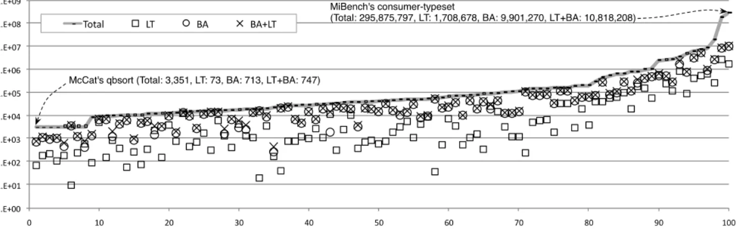
Figure 8 shows the results of the three alias analyses when applied on the 100 largest benchmarks in the LLVM test suite. We have removed the benchmark TSVC from this lot, because its 36 programs were giving us the same numbers. This fact occurs because they use a common code base. Our method rarely disambiguates more pairs of pointers than BA. Such result is expected: most of the queries consist of pairs of pointers derived from different memory allocation sites, which BA disambiguates, and we do not analyze. The ISO C Standard prohibits comparisons between two references to separately allocated objects [18]{§6.5.8p5}, even though they are used in practice [22, p.4].
Nevertheless, Figure 8 still lets us draw encouraging con-clusions. There exist many queries that we can solve, but
1.E+00 1.E+01 1.E+02 1.E+03 1.E+04 1.E+05 1.E+06 1.E+07 1.E+08 1.E+09 0 10 20 30 40 50 60 70 80 90 100
Total LT BA BA+LT
McCat's qbsort (Total: 3,351, LT: 73, BA: 713, LT+BA: 747)
MiBench's consumer-typeset
(Total: 295,875,797, LT: 1,708,678, BA: 9,901,270, LT+BA: 10,818,208)
Figure 8. Effectiveness of our alias analysis (LT), when compared to LLVM’s basic alias analysis on the 100 largest benchmarks in the LLVM test suite. Each point in the X-axis represents one benchmark. The Y-axis represents total number of queries (one query per pair of pointers), and number of queries in which each algorithm got a “no-alias” response.
Benchmark # Queries BA LT BA + LT lbm 31,944 5.90% 10.15% 15.74% mcf 49,133 15.28% 8.95% 16.52% astar 95,098 45.54% 16.05% 47.66% libq 146,301 51.64% 3.45% 52.67% sjeng 428,082 70.64% 2.03% 71.64% milc 808,471 31.05% 23.90% 43.88% soplex 1,787,190 21.43% 12.48% 23.53% bzip2 2,472,234 21.48% 23.09% 26.70% hmmer 2,574,217 8.79% 4.48% 9.38% gobmk 3,492,577 48.49% 22.91% 63.33% namd 3,685,838 22.59% 0.93% 22.76% omnetpp 12,943,554 18.71% 0.46% 18.81% h264ref 20,068,605 12.86% 1.29% 13.16% perl 23,849,576 9.92% 3.87% 10.19% dealII 37,779,455 75.05% 20.21% 75.46% gcc 186,008,992 4.26% 1.47% 4.65%
Figure 9. Comparison between three alias analyses in SPEC 2006. “# Queries” is the total number of queries per-formed when testing a given benchmark. Percentages show the ratio of queries that yield“no-alias”, given a certain alias analysis. The higher the percentage, the more precise is the pointer disambiguation method. We have highlighted the cases in which our less-than check has increased by 10% or higher the precision of LLVM’s basic alias analysis.
BA cannot. For the entire LLVM test suite, our analysis (referred as LT), increases the precision of BA by 9.49% (56,192,064 vs 59,184,181 no-alias responses). Yet, in pro-grams that make heavy use of pointer arithmetics, our results are even more impressive. For instance, in SPEC’s lbm we disambiguate 11,881 pairs of pointers, whereas BA provides precise answers to only 1,888. And, even in situations where LT falls behind BA, the former can increase the precision of the latter non-trivially. As an example, in SPEC’s gobmk, LT
returns 852,368 “no-alias” answers and BA 1,705,559. Yet, these sets are mostly disjoint: the combination of both anal-yses solves 2,274,936 queries: an increase of 34% over BA. Figure 9 summarizes these results for SPEC 2006.
How do we compare against Andersen’s analysis? Ander-sen’s [3] alias analysis is the quintessential pointer disam-biguation technique. At the time of this writing, the most up-to-date version of LLVM did not contain an implementation of such technique. However, there exist algorithms available for LLVM 4.0, which are not yet part of the official distribu-tion, such as Sui’s [35] or Chen’s [9]. We have experimented with the latter. Henceforth, we shall call it CF, because it uses context free languages (CFL) to model the inclusion-based resolution of constraints, as proposed by Zheng and Rugina [47], and by Zhang et al. [45]. A detailed descrip-tion of Chen’s implementadescrip-tion is publicly available1.
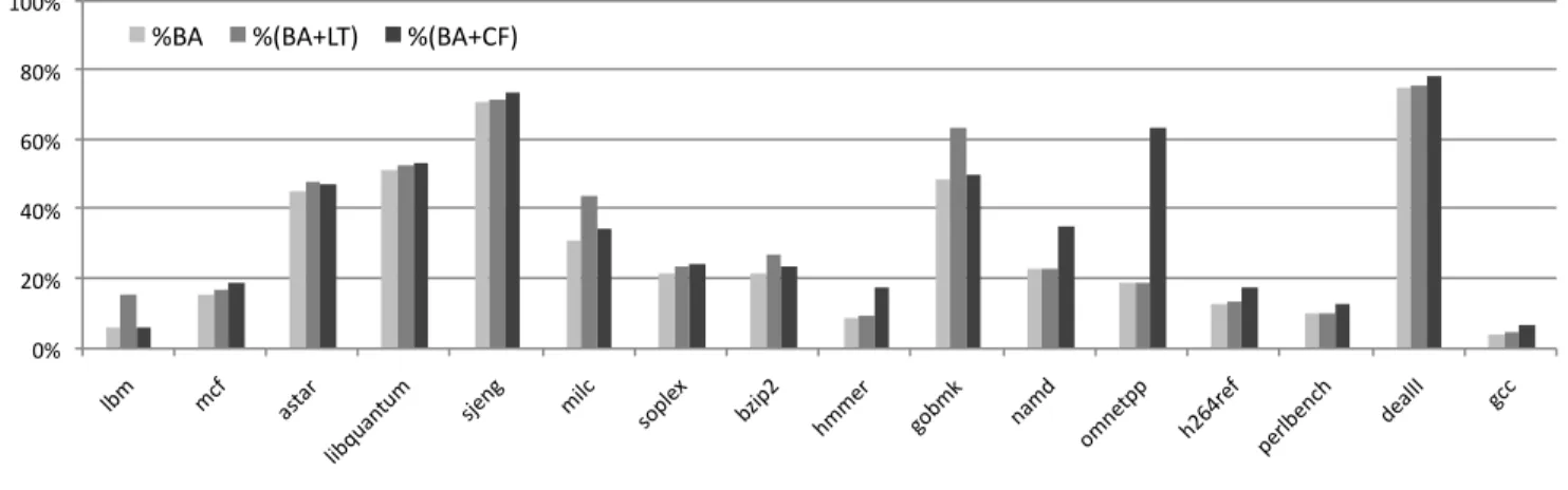
Figure 10 compares our analysis and Andersen’s. Our numbers have been obtained in LLVM 3.7, whereas CF’s has been produced via LLVM 4.0. We emphasize that both versions of this compiler produce exactly the same number of alias queries, and, more importantly, BA outputs exactly the same answers in both cases. This experiment reveals that there is no clear winner in this alias analysis context. BA+LT is more than 20% more precise than BA+CF in three benchmarks: lbm, milc and gobmk. BA+CF, in turn, is three times more precise in omnetpp. The main conclusions that we draw from this comparison are the following: (i) these analysis are complementary; and (ii) mainstream compilers still miss opportunities to disambiguate alias queries. 4.2 Scalability
We claim that the less-than analysis that we introduce in this paper presents – in practice – linear complexity on the size
0% 20% 40% 60% 80% 100% lbm mcf astar libqu antum
sjeng milc soplex bzip2 hmme r gobm k namd omne tpp h264 ref perlbe nch dealII gcc %BA %(BA+LT) %(BA+CF)
Figure 10. How two different alias analysis (LT and CF) increase the capacity of LLVM’s basic alias analysis (BA) to disambiguate pointers. The Y-axis shows the percentage of no-alias responses. The higher the bar, the better.
of the target program. Size is measured as the number of in-structions present in the intermediate representation of said program. In this section we provide evidence that corrobo-rates this claim. Figure 11 relates the number of constraints that we produce for a program, using the rules in Figure 7, with the number of instructions in that program. We show results for our 50 largest benchmarks, in number of instruc-tions, taken from SPEC and the LLVM test suite. The strong linear relation between these two quantities is visually ap-parent in Figure 11. And, going beyond visual clues, the co-efficient of determination (R2) between constraints and
in-structions is 0.992. The closer to 1.0 is R2, the stronger the
evidence of a linear behavior.
1.E+03 1.E+04 1.E+05 1.E+06 0 10 20 30 40 50 Number of Constraints Number of Instruc<ons
McCat/18-imp, 3,389 instrs, 1,219 constrs SPEC/403.gcc 918,664 instrs, 313,032 constrs
Figure 11. Comparison between the number of instructions and the number of constraints that we produce (using rules in Figure 7) per benchmark. X-axis represents benchmarks, sorted by number of instructions. The coefficient of determi-nation (R2) between these two metrics is 0.992, indicating a strong linear correlation.
As Figure 11 shows, the number of constraints that we produce is linearly proportional to the number of instructions that these constraints represent. But, what about the time to solve such constraints – is it also linear on the number
of instructions? To solve constraints, we compute the tran-sitive closure of the “less-than” relation between program variables. We use a cubic algorithm to build the transitive closure [25]. When fed with our benchmarks, this algorithm is likely to show linear behavior: the coefficient of determi-nation between the number of constraints for all our bench-marks, and the runtime of our analysis is 0.988. This linear-ity surfaces in practice because most of the constraints enter the worklist at most twice. For instance, SPEC CPU 2006, plus the 308 programs that are part of the LLVM test suite give us 8,392,822 constraints to solve. For this lot, we pop the worklist 17,800,102 times: a ratio that indicates that each constraint is visited 2.12 times until a fixed point is achieved. We emphasize that our implementation still bears the sta-tus of a research prototype. Its runtime is far from being competitive, because, currently, it relies heavily on C++’s standard data-structures, instead of using data-types more customized to do static analyses. We use std::set to rep-resent LT sets, std::map to bind LT sets to variables, and std::vector to implement the worklist. Therefore, our im-plementation still has much room to improve in terms of run-time. For instance, we took 340 seconds to solve all the less-than relations between all the scalar variables found in the 16 programs of SPEC CPU that the LLVM’s C frontend com-piles on an 2.4GHz Intel Core i7. We have already observed that most of the LT sets end up empty, and that the vast ma-jority of them, over 95%, contain only two or less elements. We intend to use such observations to improve the runtime of our analysis as future work.
4.3 Applicability
One way to measure the applicability of an alias analysis is to probe how it improves the quality of some compiler op-timization, or the precision of other static analyses. In this work, we have opted to follow the second road, and show how our new alias analysis improves the construction of the Program Dependence Graph (PDG), a classic data structure
1 20 400
0 20 40 60 80 100 120
Sta+c Loca+ons BA BA+LT
Figure 12. Precision of dependence graph. The X-axis shows benchmarks, sorted by number of static memory ref-erences in the source code. Y-axis shows number of memory nodes in the Program Dependence Graph. The more memory nodes the PDG contains, the more precise it is.
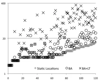
introduced by Ferrante et al. [13]. We use the implemen-tation of PDGs available in the FlowTracker system [29], which has a distribution for LLVM 3.7. The PDG is a graph whose vertices represent program variables and memory lo-cations, and the edges represent dependences between these entities. An instruction such as a[i] = b creates a data de-pendence edge from b to the memory node a[i]. The more memory nodes the PDG contains, the more precise it is, be-cause if two locations alias, they fall into the same node. In the absence of any alias information, the PDG contains at most one memory node; perfect alias information yields one memory node for each independent location in the program. It is not straightforward to compare LLVM’s basic alias analysis against our less-than-based analysis, because the former is intra-procedural, whereas the latter is inter-proce-dural. Therefore, BA ends up creating at least one mem-ory node per function that contains a load or store opera-tion present in the target program. LT, on the contrary, joins nodes that exist in the scope of different functions if it cannot prove that they do not overlap. In order to circumvent this shortcoming, we decided to use Csmith [43]. Csmith pro-duces random C programs that conform to the C99 standard, using an assortment of techniques, with the goal to find bugs in compilers. Csmith has one important advantage to us: we can tune it to produce programs with a single function, in addition to the ever present main routine. By varying the seed of its random number generator, we obtain programs of various sizes, and by varying the maximum nesting depth of pointers, we obtain a rich diversity of dependence graphs. Figure 12 shows the results that we got in this experiment.
Our alias analysis improves substantially the precision of LLVM’s BA. We have produced 120 random programs,
whose size vary from 50 to 4,030 lines. In total, the 120 PDGs produced with BA contain 1,299 memory nodes. When combined, BA and LT yield 8,114 nodes, an increase of 6.23x. We are much more precise than BA because the programs that Csmith produces do not read input values: they use constants instead. Because almost every memory indexing expression is formed by constants known at compi-lation time, LT can distinguish most of them. Although arti-ficial, this experiment reveals a striking inability of LLVM’s current alias analyses to deal with pointer arithmetics. None of the other alias analyses available in LLVM 3.7 are able to increase the precision of BA – not even marginally. Al-though we have not used CF in this experiment – it is not available for LLVM 3.7 – we speculate, from reading its source code, that it will not be able to change this scenario.
Notice that our results do not depend on the nesting depth of pointers. Our 120 benchmarks contain 6 categories of pro-grams, which we produced by varying the nesting depth of pointers from 2 to 7 levels. Thus, we had 20 programs in each category. A pointer to int of nesting depth 3, for in-stance, is declared as int***. All these programs, regardless of their category, present an average of six static memory al-location sites. On average, BA produces PDGs with 11 mem-ory nodes, independent on the bucket, and BA+LT produce PDGs with 68. The greater the number of static memory al-location sites, the better the results of both BA and LT. The largest PDG observed with BA only has 52 memory nodes (and 88 nodes if we augment BA with LT). The largest graph produced by the combination of BA and LT has 342 nodes (and only 15 nodes if we use BA without LT).
5.
Related Work
The insight of using a less-than dataflow analysis to dis-ambiguate pointers is an original contribution of this pa-per. However, such a static analysis is not new, having been used before to eliminate array bound checks. We know of two different approaches to build less-than relations: Lo-gozzo’s [20, 21] and Bodik’s [7]. Additionally, there exist non-relational analyses that produce enough information to solve less-than equations [11, 23]. In the rest of this section we discuss the differences between such work and ours. The ABCD Algorithm. The work that most closely resem-bles ours is Bodik et al.’s ABCD (short for Array Bounds Checks on Demand) algorithm [7]. Similarities stem from the fact that Bodik et al. also build a new program represen-tation to achieve a sparse less-than analysis. However, there are five key differences between that approach and ours. The first difference is a matter of presentation: Bodik et al. pro-vide a geometric interpretation to the problem of building less-than relations, whereas we adopt an algebraic formal-ization. Bodik et al. keep track of such relations via a data-structure called the inequality graph. This graph is implicit in our approach: it appears if we create a vertex vi to
from v1to v2if, and only if, v1∈ LT(v2). The weight of an
edge is the difference v2− v1, whenever known statically.
The other four differences are more fundamental.
Bodik et al. use a different algorithm to prove that a vari-able is less than another. In the absence of cycles in the in-equality graph, their approach works like ours: a positive path between vi to vj indicates that xi < xj. This path is
implicit in the transitive closure that we produce after solv-ing constraints. However, they use an extra step to handle cycles, which, in our opinion, makes their algorithm diffi-cult to reason about. Upon finding a cycle in the inequal-ity graph, Bodik et al. try to mark this cycle as increasing or decreasing. Cycles always exist due to φ-functions. De-creasing cycles cause φ-functions to be abstractly evaluated with the minimum operator applied on the weights of in-coming edges; increasing cycles invoke maximum instead. Third, Bodik et al. do not use range analysis. This is under-standable, because ABCD has been designed for just-in-time compilers, where runtime is an issue. Nevertheless, this lim-itation prevents ABCD from handling instructions such as x1 = x2+ x3 if neither x2 nor x3 are constants. Fourth,
Bodik et al.’s program representation does not split the live range of x3at an instruction such as x1= x2− x3, x3> 0.
This implementation detail lets us know that x2 > x1.
Fi-nally, we chose to compute a transitive closure of less-than relations, whereas ABCD works on demand.
The Pentagon Lattice. Logozzo and F¨ahndrich have pro-posed the Pentagon Lattice to eliminate array bound checks in type safe languages such as C#. This algebraic object is the combination of the lattice of integer intervals and the less-than lattice. Pentagons, like the ABCD algorithm, could be used to disambiguate pointers like we do. Nevertheless, there are differences between our algorithm and Logozzo’s. First, the original work on Pentagons describe a dense anal-ysis, whereas we use a different program representation to achieve sparsity. Contrary to ABCD, the Pentagon analysis infers that x2> x1given x1= x2− x3, x3> 0 like we do,
albeit on a dense fashion. Second, Logozzo and F¨ahndrich build less-than and range relations together, whereas our analysis first builds range information, then uses it to com-pute less-than relations. We have not found thus far examples in which one approach yields better results than the other; however, we believe that, from an engineering point of view, decoupling both analyses leads to simpler implementations. Fully-Relational Analyses. Our less-than analysis, ABCD and Pentagons are said to be semi-relational, meaning that they associate single program variables with sets of other variables. Fully-relational analysis, such as Octogons [23] or Polyhedrons [11], associate tuples of variables with ab-stract information. For instance, Min´e’s Octogons build re-lations such as x1 + x2 ≤ 1, where x1 and x2 are
vari-ables in the target program. As an example, Polly-LLVM2 2Available at http://polly.llvm.org/
uses fully-relational techniques to analyze loops. Polly’s de-pendence analysis is able to distinguish v[i] and v[j] in Figure 1 (a), given that j − i ≥ 1; however, it cannot analyze v[i] and v[j] in Figure 1 (b). These analyses are very pow-erful; however, they face scalability problems when dealing with large programs. Whereas a semi-relational sparse anal-ysis generates O(|V|) constraints, |V| being the number of program variables, a relational one might produce O(|V|k),
k being the number of variables used in relations.
Range-Based Alias Analyses There exist several different pointer disambiguation strategies that associate ranges with pointers [2, 4, 5, 24, 27, 31, 32, 37, 39, 41]. They all share a common idea: two memory addresses p1+ [l1, u1] and
p2+ [l2, u2] do not alias if the intervals [p1+ l1, p1+ u1]
and [p2+ l2, p2+ u2] do not overlap. These analyses differ
in the way they represent intervals, e.g., with holes [4, 37] or contiguously [2, 32]; with symbolic bounds [24, 27, 31] or with numeric bounds [4, 5, 37], etc. None of these previous work is strictly better than ours. For instance, none of them can disambiguate v[i] and v[j] in Figure 1 (b), because these locations cover regions that overlap, albeit not at the same time. Nevertheless, range based disambiguation meth-ods can solve queries that our less-than approach cannot. As an example, we are unable to disambiguate p1and p2, given
these definitions: p1= p + 1 and p2= p + 2. We know that
p < p1and p < p2, but we do not relate p1and p2.
6.
Conclusion
This paper has introduced a new technique to disambiguate pointers, which relies on a less-than analysis. Our new alias analysis uses the observation that if p1and p2are two
point-ers, such that p1 < p2, then they cannot alias. Even though
this observation is obvious, it has not been used before as the cornerstone of an alias analysis. Testimony of this state-ment is the fact that our analysis has been able to improve the precision of LLVM’s standard suite of pointer disambigua-tion techniques by a large factor in some benchmarks. There are several ways in which our idea can be further developed. One future avenue that is particularly appealing to us con-cerns speed. Currently, our research prototype can handle large programs, but its runtime is not practical: it takes sev-eral minutes to produce the transitive closure of the less-than relation for our largest benchmarks. We believe that better al-gorithms can improve this scenario substantially. The design of such algorithms is a problem that we leave open.
Acknowledgment
This project is supported by CNPq, Intel (The eCoSoC grant), FAPEMIG (The Prospiel project), and by the French National Research Agency – ANR (LABEX MILYON of Universit´e de Lyon, within the program “Investissement d’Avenir” (ANR-11-IDEX-0007)). We thank the CGO ref-erees for the very insightful comments and suggestions.
References
[1] A. V. Aho, M. S. Lam, R. Sethi, and J. D. Ullman. Compilers: Principles, Techniques, and Tools (2nd Edition). Addison Wesley, 2006.
[2] P. Alves, F. Gruber, J. Doerfert, A. Lamprineas, T. Grosser, F. Rastello, and F. M. Q. a. Pereira. Runtime pointer disam-biguation. In OOPSLA, pages 589–606. ACM, 2015. [3] L. O. Andersen. Program Analysis and Specialization for the
C Programming Language. PhD thesis, DIKU, University of Copenhagen, 1994.
[4] G. Balakrishnan and T. Reps. Analyzing memory accesses in x86 executables. In CC, pages 5–23. Springer, 2004. [5] G. Balatsouras and Y. Smaragdakis. Structure-sensitive
points-to analysis for C and C++. In SAS, pages 84–104. Springer, 2016.
[6] J. P. Banning. An efficient way to find the side effects of procedure calls and the aliases of variables. In POPL, pages 29–41. ACM, 1979.
[7] R. Bodik, R. Gupta, and V. Sarkar. ABCD: eliminating array bounds checks on demand. In PLDI, pages 321–333. ACM, 2000.
[8] Z. Budimlic, K. D. Cooper, T. J. Harvey, K. Kennedy, T. S. Oberg, and S. W. Reeves. Fast copy coalescing and live-range identification. In PLDI, pages 25–32. ACM, 2002.
[9] J. Chen. CFL alias analysis, 2016. Google’s Summer of Code Report.
[10] P. Cousot and R. Cousot. Abstract interpretation: a unified lattice model for static analysis of programs by construction or approximation of fixpoints. In POPL, pages 238–252. ACM, 1977.
[11] P. Cousot and N. Halbwachs. Automatic discovery of linear restraints among variables of a program. In POPL, pages 84– 96. ACM, 1978.
[12] R. Cytron, J. Ferrante, B. Rosen, M. Wegman, and K. Zadeck. Efficiently computing static single assignment form and the control dependence graph. TOPLAS, 13(4):451–490, 1991. [13] J. Ferrante, J. Ottenstein, and D. Warren. The program
de-pendence graph and its use in optimization. TOPLAS, 9(3): 319–349, 1987.
[14] S. Hack, D. Grund, and G. Goos. Register allocation for programs in SSA-form. In CC, pages 247–262. Springer-Verlag, 2006.
[15] B. Hardekopf and C. Lin. The ant and the grasshopper: fast and accurate pointer analysis for millions of lines of code. In PLDI, pages 290–299. ACM, 2007.
[16] B. Hardekopf and C. Lin. Flow-sensitive pointer analysis for millions of lines of code. In CGO, pages 265–280, 2011. [17] M. Hind. Pointer analysis: Haven’t we solved this problem
yet? In PASTE, pages 54–61. ACM, 2001.
[18] ISO-Standard. 9899 - The C programming language, 2011. [19] C. Lattner and V. S. Adve. LLVM: A compilation framework
for lifelong program analysis & transformation. In CGO, pages 75–88. IEEE, 2004.
[20] F. Logozzo and M. Fahndrich. Pentagons: a weakly relational abstract domain for the efficient validation of array accesses. In SAC, pages 184–188. ACM, 2008.
[21] F. Logozzo and M. F¨ahndrich. Pentagons: A weakly relational abstract domain for the efficient validation of array accesses. Sci. Comput. Program., 75(9):796–807, 2010.
[22] K. Memarian, J. Matthiesen, J. Lingard, K. Nienhuis, D. Chis-nall, R. N. M. Watson, and P. Sewell. Into the depths of C: Elaborating the de facto standards. In PLDI, pages 1–15. ACM, 2016.
[23] A. Min´e. The octagon abstract domain. Higher Order Symbol. Comput., 19:31–100, 2006.
[24] H. Nazar´e, I. Maffra, W. Santos, L. Barbosa, L. Gonnord, and F. M. Q. Pereira. Validation of memory accesses through symbolic analyses. In OOPSLA, pages 791–809. ACM, 2014. [25] E. Nuutila. Efficient transitive closure computation in large digraphs. Acta Polytechnica Scandinavia: Math. Comput. Eng., 74:1–124, 1995.
[26] H. Oh, W. Lee, K. Heo, H. Yang, and K. Yi. Selective context-sensitivity guided by impact pre-analysis. In PLDI, pages 475–484. ACM, 2014.
[27] V. Paisante, M. Maalej, L. Barbosa, L. Gonnord, and F. M. Quint˜ao Pereira. Symbolic range analysis of pointers. In CGO, pages 171–181. ACM, 2016.
[28] F. M. Q. Pereira and D. Berlin. Wave propagation and deep propagation for pointer analysis. In CGO, pages 126–135. IEEE, 2009.
[29] B. Rodrigues, F. M. Quint˜ao Pereira, and D. F. Aranha. Sparse representation of implicit flows with applications to side-channel detection. In CC, pages 110–120. ACM, 2016. [30] R. E. Rodrigues, V. H. S. Campos, and F. M. Q. Pereira. A
fast and low overhead technique to secure programs against integer overflows. In CGO. ACM, 2013.
[31] R. Rugina and M. C. Rinard. Symbolic bounds analysis of pointers, array indices, and accessed memory regions. TOPLAS, 27(2):185–235, 2005.
[32] S. Rus, L. Rauchwerger, and J. Hoeflinger. Hybrid analysis: Static and dynamic memory reference analysis. In ICS, pages 251–283. IEEE, 2002.
[33] T. C. Spillman. Exposing side-effects in a PL/I optimizing compiler. In IFIP, pages 376–381. Springer, 1971.
[34] B. Steensgaard. Points-to analysis in almost linear time. In POPL, pages 32–41. ACM, 1996.
[35] Y. Sui and J. Xue. SVF: Interprocedural static value-flow analysis in llvm. In CC, pages 265–266. ACM, 2016. [36] Y. Sui, P. Di, and J. Xue. Sparse flow-sensitive pointer analysis
for multithreaded programs. In CGO, pages 160–170. ACM, 2016.
[37] Y. Sui, X. Fan, H. Zhou, and J. Xue. Loop-oriented array- and field-sensitive pointer analysis for automatic SIMD vectoriza-tion. In LCTES, pages 41–51. ACM, 2016.
[38] A. L. C. Tavares, B. Boissinot, F. M. Q. Pereira, and F. Rastello. Parameterized construction of program represen-tations for sparse dataflow analyses. In Compiler Construc-tion, pages 2–21. Springer, 2014.
[39] R. A. van Engelen, J. Birch, Y. Shou, B. Walsh, and K. A. Gallivan. A unified framework for nonlinear dependence testing and symbolic analysis. In ICS, pages 106–115. ACM, 2004.
[40] J. Whaley and M. S. Lam. Cloning-based context-sensitive pointer alias analysis using binary decision diagrams. In PLDI, pages 131–144. ACM, 2004.
[41] R. P. Wilson and M. S. Lam. Efficient context-sensitive pointer analysis for c programs. In PLDI, pages 1–12. ACM, 1995.
[42] M. Wolfe. High Performance Compilers for Parallel Comput-ing. Adison-Wesley, 1st edition, 1996.
[43] X. Yang, Y. Chen, E. Eide, and J. Regehr. Finding and understanding bugs in C compilers. In PLDI, pages 283–294. ACM, 2011.
[44] S. H. Yong and S. Horwitz. Pointer-range analysis. In SAS, pages 133–148. Springer, 2004.
[45] Q. Zhang, M. R. Lyu, H. Yuan, and Z. Su. Fast algorithms for Dyck-CFL-reachability with applications to alias analysis. In PLDI, pages 435–446. ACM, 2013.
[46] J. Zhao, S. Nagarakatte, M. M. K. Martin, and S. Zdancewic. Formal verification of ssa-based optimizations for llvm. In PLDI, pages 175–186. ACM, 2013.
[47] X. Zheng and R. Rugina. Demand-driven alias analysis for c. In POPL, pages 197–208. ACM, 2008.
A.
Artifact Evaluation
This artifact is in the form of a virtual machine and it is distributed through the link: http://cuda.dcc.ufmg. br/CGO17/strict-inequalities/. This virtual machine contains the code and execution scripts for the work pre-sented in this paper. In the desktop folder, you will find ways to run our analysis on any source code you choose, or on the benchmarks used in this paper’s evaluation.
A.1 The Code
The code from this work can be found inside LLVM’s build directory inside the virtual machine. The LLVM source and build directory is at /llvm/, and the code for the analyses are in /llvm/lib/Transforms/. In total we have used 4 passes in this paper:
•/llvm/lib/Transforms/sraa
The main pointer alias analysis presented in this paper.
•/llvm/lib/Transforms/vSSA
A pass that transforms the program to the e-SSA form, needed in order to use the Strict Relations Alias Analysis.
•/llvm/lib/Transforms/RangeAnalysis
A symbolic Range Analysis also used in the Strict Rela-tions Alias Analysis.
•/llvm/lib/Transforms/DepGraph
A pass that builds the program dependence graph. This pass is used in one of our tests, to show the effectiveness of our new alias analysis when comparing the number of memory nodes yielded by the DepGraph when running it coupled with the Strict Relations Alias Analysis. We developed our work on LLVM 3.7.
A.2 Getting Started
The artifact is provided as a Virtual Machine image. To use the artifact, you need to download and install the Vir-tualBox VM player at https://www.virtualbox.org/ wiki/Downloads. After downloading and installing Virtu-alBox, to run the VM image, you must perform the following steps:
1. Download and decompress the VM image. 2. OpenVirtualBox.
3. Create a new virtual machine, by clicking in “Machine”, “New...”.
4. Give a name to the new VM, by filling the “Name” field. 5. In “Type”, select “Linux”.
6. In “Version”, select “Ubuntu (64 bit)”.
7. Click “continue”, select the desired amount of RAM memory, then click “continue” again.
8. In the hard drive selection screen, select the option “Use an existing virtual hard drive file”, then select the .vdi file containing the VM image that you just downloaded.
9. Your Virtual Machine is ready to use! To start, simply double-click it in the VirtualBox VM list
If the VM prompts for a username and password, you may use the following combination:
•login: cgoartifact
•password: artifact A.3 Running the Examples
Inside the folder ExecuteExamples you may find a script to compile any C code and run our analysis. If you wish to compile a program, you may use the script compile.sh and pass as first parameter the name of the program you wish to compile. For example, say you want to compile the program test.c:
$ bash compile.sh test
You may omit the file extension (.c) when passing the name of the program as a parameter. After the compilation, if you wish to run our Strict Relations Alias Analysis evalua-tion, you can run the script sraa.sh. The output will be the LLVM’s default alias analysis evaluation, with a thorough list of alias information on the program.
$ bash sraa.sh test
If you wish to compare it with the LLVM’s basic alias analysis alone, you can also run the script basicaa.sh on any program you wish. You may also use the script random.sh to generate a random C program with the tool Csmith:
$ bash random.sh random
The clean.sh script will remove all files created by the other scripts.
A.4 Running the Benchmarks
We have executed 3 main evaluation tests in our paper: Preci-sion, Scalability and Applicability. These tests are described in Section 4 of this paper. In the folder Benchmarks you will find the scripts to run the benchmarks used in the pa-per. You will find two folders: aaeval and memnodes. In the folder aaeval there is a script called run.sh that runs two of the 3 evaluation tests we ran in our paper, the tests of Precision and Scalability. Both tests are executed on the LLVM’s test-suite and on the SpecCPU2006. The test of Pre-cision evaluates how better our alias analysis is compared to the Basic Alias Analysis provided by LLVM. So it runs the basicaa, the sraa and both together on the entire test-suite. The test of Scalability evaluates the growth of the number of constraints generated during the Strict Relations Alias Anal-ysis compared to the size of the programs being analyzed. The script run.sh will basically run the tests on the entire test-suite and copy the .csv files containing the statistics to the folder aaeval. At the end of the execution you may find
the .csv files in the folder. Warning: Bear in mind that the tests may take a while (up to 4 hours), mainly because they are running on a virtual machine.
In the folder memnodes you may find another script called run.sh that executes the third test in our paper, the test of Applicability. The test of Applicability runs a dence Graph pass that generates a PDG (Program Depen-dence Graph) and counts the number of memory nodes in it. Our aim is to show that our new alias analysis yields more memory nodes in these graphs, because it is more pre-cise. We also run this test in the entire test-suite plus SPEC-Cpu2006. In order to do improve our evaluation, we used the tool Csmith to generate 120 random C programs and then we ran the Dependence Graph coupled with our Strict Rela-tions Alias Analysis in all of them. We showed that the PDG generated without our analysis has less memory nodes than the PDG generated with our alias analysis. The random gen-erated C programs are in the folder SingleSource, inside the LLVM’s test-suite root, so this test already evaluates the entire test-suite and the random generated programs as well.
To use csmith to generate a random program, use the script random.sh in the folder ExecuteExamples.
A.5 The Output
The output for our analysis is very simple. We use the aa-eval pass to compare, within the same function, all possible pairs of pointers and then we return how many comparisons issued a NoAlias, MayAlias or a MustAlias response. Regarding the Dependence Graph, we basically count the number of Memory Nodes yielded. The output for this analysis is formatted in CSV files. When you run the tests with the script run.sh, the CSV files will be copied to your working directory.
Reviewing Methodology
This artifact has been reviewed according to the guide-lines established by the Artifact Evaluation Committee of CGO and PPoPP. The reviewing methodology is described
in http://cTuning.org/ae/submission-20161020.