A Mixture Approach for Semisolid Metal Mold Filing Simulation

Publisher’s version / Version de l'éditeur:

L’accès à ce site Web et l’utilisation de son contenu sont assujettis aux conditions présentées dans le site

The 11th International Conference on Modeling of Casting, Welding and

Advanced Solidification Processes [Proceedings], 2006-06

READ THESE TERMS AND CONDITIONS CAREFULLY BEFORE USING THIS WEBSITE.

https://nrc-publications.canada.ca/eng/copyright

NRC Publications Archive Record / Notice des Archives des publications du CNRC :

https://nrc-publications.canada.ca/eng/view/object/?id=0a21a755-0b09-4ad7-9bd6-30634f34c1e1 https://publications-cnrc.canada.ca/fra/voir/objet/?id=0a21a755-0b09-4ad7-9bd6-30634f34c1e1

NRC Publications Archive

Archives des publications du CNRC

This publication could be one of several versions: author’s original, accepted manuscript or the publisher’s version. / La version de cette publication peut être l’une des suivantes : la version prépublication de l’auteur, la version acceptée du manuscrit ou la version de l’éditeur.

Access and use of this website and the material on it are subject to the Terms and Conditions set forth at

A Mixture Approach for Semisolid Metal Mold Filing Simulation

Pineau, F.; Ilinca, F.; Hétu, J. F.

f

I

I I I I

I

I

I

I

I I

I

I

I

I

I

i

rn i 2005

-

I I \ Q'2 2

-.9

c. N RC.

~

'O~Ll3

Proceedings of MCWASP 2006 Edited by

TMS (The Minerals, Metals & Materials Society), 2006 I

I I I I I I I I I

A MIXTURE

APPROACH

FOR SEMISOLID

METAL MOLD

FILLING SIMULATIONS

F. Pineau!, F. Ilinca2, J.F. Hetu2

1Aluminium Technology Centre, National Research Council, 501 Universite Blvd East, Chicoutimi, Que, G7H 8C3, Canada

2Industrial Material Institute, National Research Council, 75 de Mortagne Blvd., Boucherville, Que, J4B 6Y4, Canada

Keywords: Two-phase flow, Mixture approach, Finite Element

Abstract

I

I

I

I

I

I

I

I

I

I

I

I

I

I

I

I

I

I

I

Semisolid metal alloys have a special micro-structure of globular grains suspended in a liquid metal matrix. This particular physical state of the matter can be exploited to produce near-net-shape parts with improved mechanical properties. However, the behavior of the slurry is strongly influenced by the local solid fraction and state of agglomeration. Different flow instabilities associated with the combined flow and solidification process result, which complicate the application of semisolid processing in the casting industry. So far, most of the semisolid theory has been derived from experimental data, which are somewhat difficult to obtain. To reproduce some features of semisolid flows, a two-phase numerical model based on the mixture theory is developed. The hydrodynamic part of the model is written in the same form as for most incompressible CFD codes but, the velocity field represents velocities of the mixture. A source term is added to the momentum equations to take into account the diffusion velocities of the individual phases. The relative velocity between the liquid and solid phases is obtained from an algebraic relation related to the interaction forces between the phases. The effective viscosity of the material is given by a Cross model derived from experimental rheological data. The paper describes the model development and its implementation in the Industrial Material Institute finite element code. Calculations are performed for a classical configuration of interest in thixocasting. Though the Darcy model used to approximate the interaction forces has some drawbacks, realistic segregation patterns are obtained and discussed.

Introduction

Using semisolid metal processes allows production of structural parts with superior mechan-ical properties compared to those produced using conventional casting methods. This is due to the characteristic rheology of the feed stock material whose state lies between that of a solid and a liquid; at rest, the material maintains its structural integrity but when sheared, it flows with relative ease. Because of its higher viscosity, the material fills a mold in a progressive manner, thus eliminating gas entrapment and defects. But the presence of two distinct phases sometimes gives rise to surprising behaviors because of a change in local ef-fective properties due to segregation. The latter can also affect the homogeneity of the final part. In view of problems encountered in the industrial application of semisolid metal, it is necessary to gain better understanding of this particular state of matter. Since experimental

n -I I

I

I

I

I

I

I

I

I

I

I

I

I

measurements for such partially molten material flows are difficult to perform, because of the extreme conditions of temperature and pressure, significant improvements can be envisioned through proper numerical simulations and computer aided control of these technologies. A finite element two-phase mixture model is thus presented to attempt to reproduce some features of these complex flows.

Mixture Flow Conservation Equations

I

I

I

I

I

I

I

I

The bulk behavior of semisolid slurries has long been studied by using single-phase averaged models, but these approaches do not account for the phase segregation within the material. To get a better understanding of the process, a multiphase approach is needed. Physically, such multiphase system can be formulated in terms of the local instantaneous variables associated to each phase and for which boundary conditions at the phase interfaces must be matched. However, obtaining a solution from these formulations could be very difficult and even impossible because of the multiple scales involved. To make the problem more tractable, spatial averaged balance equations of the mixture at the scale of an elementary volume (macroscopic scale) are often employed. Details concerning the averaging methods and their relevance to the different conservation equations can be found for example in reference [1]. Another alternative is to regard the whole particle-fluid combination as a single flowing continuum with effective macroscopic properties (mixture model). Each phase is then represented by a species concentration equation, which is formulated in such a way, as to allow migration of the species throughout the bulk flow. A source term added to the momentum equation accounts for phase diffusion velocities in the mixture. The diffusion velocities are then obtained from the relative velocities between the phases which are calculated from a balance of forces acting on each phase.

Model Equations

Three-dimensional modeling of the flow of a two-phase mixture is based on conservation of mass, momentum and solid volume fraction for an incompressible fluid. Derivation of the mixture conservation equations are detailed in reference [2]. The mixture density is given by

Pm

= asps+aIPI,whereas and al are respectivelythe solid and liquidvolumefractions. Note

that as + al

=

1. The mixture velocity Um is the mass-weighted average of the constituent

velocities (k

= t,

s):

1

Um

=

- LakPkuk

Pm k

For the sake of simplifying the equations, the same value for the liquid and solid phase

densities is taken (Ps

=

PI

=

Pm

=

constant), although we know that for Aluminium A356

alloys, there is about 7% difference. We assume that the volume solid fraction is lower than the maximum packing fraction in most of the filling process and thus the phase pressures are

the same (PI

=

Ps

=

Pm)' Neglecting the body forces, the mass conservation and momentum

I

I

I

I

I

I

I

I

I

I

I

I Uml

=

-asuls

(5)

(6)

(7)

I

I

I

I

I

I

I

I

I

I

I

I TDm

=

Pm[asumsums+ (1

-

as)umlumd

Ums

=

(1 - as) Uls

Tmis the average viscous stress and TDm is the diffusion stress due to the phase slip. Ums,

Umlare respectively the solid and liquid phase diffusion velocities. Each of them represents

the drifting motion relative to the centre of mass of the mixture, identified as a point moving with the mixture velocity Um. As for Uls, it stands for the relative velocity between the solid and liquid phases, (Uls = Us - Ul).

In addition to the flow equations (2),(3), the solid phase continuity equation written in

terms of the mixture variables is solved for as, the solid phase volume fraction (e.g. [2]).

I

I

I

I

I

I

I

I 8 (as)

Pm8i + Pm\7. (asum)

=

-Pm\7. (asums) (8) One possible difficulty in the numerical treatment of two-phase flows lies in ensuring that the volume fraction for each phase remains between a and 1. Failure to ensure this realizability condition results in non-physical solutions and can affect the solution process. For example a zero value of the solid fraction as gives an infinite value of the permeability coefficient which in turn determines an infinite value of the relative velocity between the solid and liquid phases. One way of enforcing the realizability condition is to use solution clipping and limiters. It is a robust approach in the sense that the condition can be enforced at every time step or every iteration and it can be applied to almost any numerical algorithm. However, it does have two drawbacks. First, it slows down the convergence of the iterative solver because clipping implies local change of the solution with the effect of deteriorating the residual of the equation. Secondly, clipping introduces noise and oscillations in the solution fields. In this work we perform a change of variable having the effect of enforcing the volume fraction to remain between a and 1. A similar approach was used in reference [3] for the solution of two-equation turbulence models for which turbulence variables must be positive.

Change of Variable for the Solid Phase Equation

The continuity equation for the solid fraction in the case of an incompressible mixture and with no change of phase is:

88~s+ Um. \7as + \7 . (asums)

=

a

(9)

One way to enforcethat as remains in the a to 1 range is to make the followingchange

of dependent variable:

as

=

~ In

C ~saJ

(10)

The new dependent variable as is definedonly if as lies betweena and 1. When solving

for as, the solid fraction is obtained from

1 ea.

as = [1+ tanh(as)] =

-2 ea.+ e-a.

which will always satisfy the realizability condition. The transport equation for as is obtained by first rewriting equation (9) by using equation (6) for the diffusion velocity of the solid phase:

(11)

88~s+ Um . \7as + Ums . \7as + as(1 - as)\7 . Uls + asuls . \7(1 - as)

= a

(12)

I I I I I I I I I I I I

I

I I I I I I I

Taking V'(1

- as)

= -V'as equation (12) becomes:

a~s + rUm+ Ums

-

asuls] . V'as + as(1- as)V' . Uls = 0 (13)

It now suffice to divide equation (13) by 2as(1- as) and to use the following identities: 1 aas aas

2as(1- as) at - at '

1

-V'as = V'as

(14)

to finally obtain the equation for the new dependent variable as:

a~

[

1

at + Um+Ums-asUls].V'as+2V'.UIS=0

(15)

Once as is computed, the solid fraction is determined from equation (11). Note that solving for as is equivalent to the original model equation for the solid fraction. Hence, there is no change in the mixture model. The only modification is that the computational variables are now enforcing implicitly the realizability condition.

Closures

The interaction force between the phases is a key area of research for semi-solid metal ap-plications as it determines the relative velocity between the phases. For now, the slurry is viewed as a fluid saturated isotropic porous media. In that case, the phase interaction term that appears in the momentum equations of each phase is given by reference [4]:

alILI

Ml

=

-Ms = PIV'al +

K

(us

- Ul) (16)

where K is the permeability of the porous media obtained from the Carman-Kozeny relation:

d; (1 - as)3

K

=

180 (as) (17)

and dp is the particle diameter. Equation (16) is then substituted in the liquid phase

mo-mentum equation to give, (assuming that PI = Pm):

a

alILI

at (aIPlul) + V'. (aIPlulul) = -alV'Pm + V'. alTI + K (us - Ul) (18)

Let's take again PI = constant = Pm, equation (18) becomes:

[

aUI aal

]

Pm al at + Ul at + alul. V'UI

+

Ul (V'al. Ul

+

a/V'. Ul) =

a/ILl

-atV'Pm

+

V'.

am + K

(us

- Ul) (19)

For semi-solid slurries, the volume solid fraction is high, (2: 0.4), and strong pressure gradients are expected. Consequently, relative velocities between the phases are assumed to depend mainly on the pressure gradient and all other terms in equation (19) are neglected:

K

(us - Ul) = -V'Pm

where f.Llis the viscosity of the liquid phase.

The rheological behavior of the slurry must also be defined. The latter remains an area of intense research in the semisolid community. The proper definition of this behavior is essential for a successful process simulation but it is still very difficult to define. In this study, a Cross model derived from a shear rate step change experiment [5],modified to also account for solid fraction variations, is employed for the effective viscosity of the mixture:

f-£eff

=

[ f-£oo+ f.Lo- /100 ]

(

(as - as

)

)

-2.5amp

1 + (k-y)l-n 1 - ampref (21)

with n = 0.282, k = 6.46, f-£o= 10000, f.L00= 0.05, amp = 0.65, aSref = 0.4 and -y is the shear

rate.

Front Tracking Approach

A level-set technique is finally employed to capture the position of the flow front [6]. The level-set approach defines a smooth function F(x, t) such that a critical value Fe represents the position of the interface. The pseudo-concentration function is convected using the mixture velocity field provided by the solution of the mixture conservation equations.

8F

7it+um.\lF=O

(22) I I I I I I I Boundary Conditions

Setting the boundary conditions completes the statement of the problem. On the inlet section of the mold, both the mixture velocity and volume solid fraction are set. The latter corresponds to usual solid volume fraction found in semisolid processing and is related to the initial temperature of the material. Either non-slip boundary conditions or specification of surface stresses are imposed on the filled cavity walls, while the shear stress on the mold surface is considered to be zero in the unfilled part.

Numerical Implementation

The proposed formulation is implemented in the finite element code for mold filling applica-tions developed at the Industrial Materials Institute [6,7].

At each time step, global iterations are performed for the momentum, continuity and volume solid fraction transport equations. After convergence of the velocity-pressure equa-tions, nodal pressure gradients are recovered through a local projection method [8]. Relative velocities and diffusion velocities are then computed from the projected pressure gradient field. Finally, the front tracking equation is solved.

Application Tests

The filling of a cylindrical reservoir is used for initial tests. This simple geometrical config-uration comes from reference [9] and allows the reproduction of several features observed in

semisolid die casting. The entrance velocity is set to Uinlet

=

15,2 mls which yields a "shell

like filling mode" [10]. The initial solid fraction in the volume as well as the solid fraction

boundary condition at the inlet is set to as

=

0.4. The particle diameter din equation (17)

I I I I I I

I

I I

I

I I I

I

The mesh for this application has 30753 nodes and 145920 elements. Simulations are performed on a parallel computer using 16 processors. The computational time is about 6 hours for each case.

The first set of simulations are performed using no-slip flow boundary conditions at the walls (urn

=

0). Note that this does not mean that the individual phase velocitiesare zero

at this location, (see equation (1)). In fact, by using a Darcy approximation for the phase interaction force, the relative velocity between the phases is given by the pressure gradient field. The latter is not nil at the wall and thus yields non-zero relative phase velocities there. Convergence of the solution appears to be very difficult in this case. For this reason, the solution algorithm controls that the values of the relative velocity is not greater than the mixture velocity everywhere in the domain. So, a zero mixture velocity implies no relative velocity between the phases. However, such a model may cause some consistency problems at the walls as the divergence of the relative velocity field is altered.

Figure (1) represents a typical filling sequence. The gray spectrum changes from 0.38 (black) to 0.58 (white) solid fraction. After hitting the bottom of the reservoir, see Figure (I-a), the slurry turns radially and fills the mold backward in a "mushroom like" pattern that folds up on itself. Phase segregation occurs around the stagnation point of the impinging jet due to the strong pressure gradients that prevail there. Some of the solid is convected radially and subsequently backward. The ensuing phase distribution is then directly related to the pressure gradient field, see Figures (l-b,c). (Increasing solid fraction in the direction of the pressure gradient). Note the "higher solid fraction" ring area in the vicinity of the impinging radial jet. The pressure field and corresponding phase relative velocities for the 70% volume filled situation are depicted in Figure (2-a,b). The final solid fraction at the end of the filling is shown in Figure (I-d).

I

I

I

I

I

I

I

I

I

I I I I I I I

I

(a) 20% filled (b) 40% filled (c) 70% filled (d) 100% filled Figure 1. Solid volume fraction distributions, no-slip conditions.

In the second set of simulations, a shear stress is applied at the walls instead of the no-slip boundary condition used previously. All other simulation parameters are the same. "Partial slip" for the mixture velocity is now permitted at the mesh boundaries and so, non-zero relative velocities. The results are depicted in Figure (3) with the gray scale ranging from 0.35 (black) to 0.45 (white) solid fraction. Due to this "slip" boundary condition, the filling front as well as the solid fraction distribution are different from the previous case. The slurry fills the mold again in a "shell like manner" but it forms a loop that completely wets the boundaries before completing the filling from the exterior to the interior. Because of the slip conditions, the solid phase tends to be more evenly distributed along the walls. The final solid fraction distribution at the end of the filling stage is depicted in Figure (3-d).

These two cases emphasize the importance of the type of boundary conditions to be used in such problems. Experiments indicate that partial slip conditions are possibly more

I I I I I I I I I I I

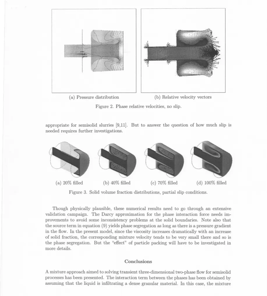
(a) Pressure distribution

I I I I I I I

Figure 2. Phase relative velocities, no slip.

(b) Relative velocity vectors

appropriate for semisolid slurries [9,11]. But to answer the question of how much slip is needed requires further investigations.

(a) 20% filled (b) 40% filled

Figure 3. Solid volume fraction distributions, partial slip conditions.

(c) 70% filled (d) 100% filled

Though physically plausible, these numerical results need to go through an extensive validation campaign. The Darcy approximation for the phase interaction force needs im-provements to avoid some inconsistency problems at the solid boundaries. Note also that the source term in equation (9) yields phase segregation as long as there is a pressure gradient in the flow. In the present model, since the viscosity increases dramatically with an increase of solid fraction, the corresponding mixture velocity tends to be very small there and so is the phase segregation. But the "effect" of particle packing will have to be investigated in more details.

Conclusions

A mixture approach aimed to solving transient three-dimensional two-phase flowfor semisolid processes has been presented. The interaction term between the phases has been obtained by assuming that the liquid is infiltrating a dense granular material. In this case, the mixture

pressure gradient is the driving force that causes the relative motion between the phases. A change of variable for the solid volume fraction conservation equation has been used and resulted in numerical solutions that always remain in the 0 to 1 range. This yields a stable solution without the use of clipping delimiters. Though the approximation yields intuitively reasonable segregation patterns, some questions have been raised. Effectively, no-slip boundary conditions are not consistent with the Darcy approximation for the relative velocity between the phases. A better approximation for the relative phase motion and the associated boundary conditions has yet to be investigated.

References

1. M. Rappaz, M. Bellet, and M. Deville, "Numerical Modeling in Materials Science and Engineering," Springer Series in Computational Mathematics, vol 32 (Berlin, Springer Verlag, 2002), 540.

2. M. Manninen and V. Taivassalo, "On the mixture model for multi phase flow," (VTT Energy, VTT, Finland, 1996).

3. F. !linca and D. Pelletier, "Positivity preservation and adaptative solution for the k-E

model of turbulence," AIAA Journal, 36 (1) (1998), 44-50.

4. R.M. Bowen, Theory of Mixtures, (New York, A.C. Eringen, 1976).

5. L. Azzy, F. Ajersch, and T.F. Stephenson, "Rheological characteristic of semi-solid grani

composite alloy," ed. G.L. Chiarmetta and M. Rosso, (Proceedings of the 6th International

Conference on Semi-Solid Processing of Alloys and Composites, Torino, Italy, 2000), 527-532.

6. F. !linca and J.F. Hetu, "Finite element solution of three-dimensional turbulent flows applied to mold-filling problems," Int. J. Numer. Meth. in Fluids, 34 (2000), 729-750.

7. M. Audet, J.F. Hetu, and F. !linca, "Application of parallel algorithm to 3-d mold filling and solidification processes," ed. B.G thomas and C. Beckermann, (Modeling of Casting,

Welding and Advanced Solidification Processes-VIII, TMS, Warrendale, PA, 1998), 29-36.

8. O.C. Zienkiewicz and J.Z. Zhu, "The superconvergent patch recovery and a posteriori error estimators. part 1: The recovery technique," Int. J. Numer. Meth. in Eng., 33 (1992),

1331-1364.

9. L. Orgeas et al., "Modelling of semi-solid processing using a modified temperature-dependent power-law model," Modelling Simul. Mater. Sci. Eng., 11 (2003), 553-574.