Computation of acoustic scattering from elastic conical shells with endcaps using the hybrid finite element/ virtual source approach

Computation of acoustic scattering from elastic conical shells

with endcaps using the hybrid finite element/ virtual source

approach

Hwee Min Charles Low

B.Eng (1998)

National University of Singapore

Submitted to the Department of Ocean Engineering in Partial Fulfillment of the Requirements for the Degree of

Master of Science in Ocean Engineering At the

Massachusetts Institute of Technology

February 2004

2004 Massachusetts Institute of Technology All rights reserved

MASSACHUSETTS INSTIlTftE OF TECHNOLOGY

SEP 0

1

2005

LIBRARIES

A uthor... ...

Department of Ocean Engineering

May 7, 2004

C ertified b y ... .. ..

Professoir Schmidt Department of Ocean Engineering Thesis Supervisor

A ccepted by ... .. ...

Professor Michael S. Triantafyllou Department of Ocean Engineering Chair, Department Committee on Graduate Studies

ABSTRACT

Studying and understanding acoustic scattering pattern from underwater targets has been of interest to various communities such as the archeologists and the navy for several reasons and applications. The present state-of-the-art technique in this area involves such methods as analytical approach and FEM/BEM numerical technique. This thesis aims to study and demonstrate the power of using the hybrid virtual source/FE approach where the physical presence of a target is replaced by virtual sources placed in the vicinity of the target and in a manner where the pressure/displacement relationship on the target surface is satisfied by the virtual sources when the target is being insonified. Accurate results for the far-field radiation of the target can be obtained by superposition of the point source Green's function of each virtual source. The hybrid virtual source/FE approach shows potential to be a computationally efficient method for computing acoustic scattering. The derivation of the dynamic flexibility matrix for an elastic conical shell with endcaps will be illustrated in this thesis. It will be shown that the dynamic flexibility matrix corresponds to the acoustic admittance matrix in the virtual source approach where the scattering functions are computed in the MIT's program OASES/SCATT. Moreover, the benchmarking and validation of the approach will be conducted with the hybrid analytical/ virtual source approach. Firstly, the approach predicts natural frequencies close to the theoretical analysis for higher order modes with more than 2 circumferential transverse vibration lobes. Secondly, it produces displacement profile that conforms to analytical results. The scattering functions are also in agreement those computed by the hybrid analytical/ virtual source approach, with discrepancies observed at lower frequencies. In exact terms, discrepancies start to appear for frequency in the range of

1000 to 2000 Hz for a 0.01m thick, 2 m long, 0.3m radius steel cylinder without endcaps.

The scattering functions will be compared with the SCATT/OASES virtual source approach for pressure release and rigid cylinders and cones. For the hybrid FE/virtual source approach, the structural sound speed and density approach zero and infinity for pressure-release and rigid target respectively. On the other hand, in the SCATT/OASES virtual source approach, the pressure and displacement are required to vanish on the target surface respectively. It will be shown that the two approaches agree with each other.

Moreover, scattering functions over steel cones and cylinders for various frequencies have also been derived in this research. The results will be interpreted physically and theoretically in this thesis. The importance of including structural damping in the finite element formulation of the target so as to reflect the effect of resonance on scattering will be illustrated. Other issues, such as effect of target orientations on scattering, will also be

investigated in this thesis.

The code has shown good potential for adaptation to compute scattering over other axi-symmteric shapes using conical shells and circular plates as building blocks and the hybrid FE/ virtual source approach.

ACKNOWLEDGEMENT

One of my most valuable rewards of coming to MIT is to stretch my modest intellect to a limit far beyond what I could imagine myself doing before coming.

One reason this has been possible is that I have the precious opportunity of working with my advisor, Henrik Schmidt, who is one of the most eminent scholars in the field of ocean acoustics. I would thus like to thank him for his guidance and patience in my research.

My second home in Boston (thankfully not my first, though) is my office in 5-007. Life

here in MIT would not be as valuable and academically rewarding if without the company of the people in 5-007: Bertrand, Wenyu Luo, Mark Rapo, Hun Joe Kim, Tai Wei Wang, who are all both my colleagues and friends.

I would also like to thank my other friends in MIT and Boston. I have the rare

opportunity of staying in graduate apartment, Tang hall 19D for my entire two years here and would like to thank those who have stayed with me for their friendship: Erico Guizzo, Fabio Rabbani and many others. My special thanks to Lisa Kang and other close friends from Boston Chinese Evangelical Church (BCEC).

My program here would not have been possible without the support of DSO National

Laboratories. My sincere thanks to Tong Boon Quek and Frank Teo for their support of my postgraduate studies and Joo Thiam Goh who have sparked my interest in ocean acoustics and for guidance in deciding what I want to pursue in MIT.

Last but not least, I would like to thank my dear family, though physically absence during my two years away from home, have given so much support.

TABLE OF CONTENTS I IN T R O D U C T IO N ... 13 1.1 B ack ground ... . . 13 1.2 L iterature R eview ... 15 1.2.1 A nalytical M ethods... 15 1.2.2 N um erical m ethods ... 15

1.2.3 Computational Acoustic Method ... 16

1.2.4 Virtual Source Approach ... 17

1.2.5 FE Modeling of axi-symmetrical shells and plates... 18

1.3 M o tivation ... . 19

1.4 R esearch O bjectives... 21

1.5 T hesis O utline ... . 23

2 T H E O R Y ... 2 5 2.1 Virtual Source Approach ... 25

2.1.1 Green's Function Matrix... 27

2.1.2 Wavefield Superposition... 29

2.2 Acoustic Boundary Conditions for axi-symmetric elastic target... 30

2.2.1 Dynamic Stiffness Matrix of Conical Shells in the 2D domain... 30

2.2.2 Dynamic Stiffness Matrix of Circular Plates in 2D domain... 32

2.2.3 Global Flexibility Matrix for conical shells with endcaps... 34

2.2.4 Admittance matrix in the 3D domain... 36

2.3 Farfield Radiation of Target... 40

3 COMPUTATIONAL RESULTS FOR ELASTIC CYLINDER ... 43

3.1 Analytical modeling of in vacuo vibration of cylinder... 43

3.2 Resonant frequencies of FE model ... 47

3.3 Response of cylinder under acoustic pressure loading ... 51

3.3.1 Displacement potential of the form n sin-ze Lcosn ... 51

N ) T 3.3.2 Displacement potential of the form V nO sin- ze 55 n=0 3.4 Acoustic Scattering from steel cylinder without endcap ... 60

3.5 Acoustic Scattering from steel cylinder with endcap ... 67

3.5.1 Rigid and Pressure Release Target Surface ... 67

3.5.2 Elastic Target Surface ... 71

3.6 Scattering from a pitched cylinder... 76

3.7 Scattering strength at resonance... 78

3.8 D iscussion ... . . 85

4 COMPUTATIONAL RESULTS FOR ELASTIC CONE... 87

4.1 Acoustic scattering from pressure release and rigid cone with endcaps... 88

4.2 Acoustic scattering from elastic cone with endcaps ... 92

4 .3 D iscussion ... . . 95

5 C O N C LU SIO N S... 97 . 97

5.2 Research objectives ... 98 5.3 Future work ... 100 6 BIBLIOGRAPHY ... 101 7 APPEND IX A ... 103 8 APPEND IX B ... 105 9 APPEND IX C ... 107 10 APPEND IX D ... 109

LIST OF FIGURES

Figure 1-1 A summary of various techniques for computing acoustic scattering ... 19

Figure 2-1 Virtual source representation of target ... 25

Figure 2-2 C onical shell elem ent ... 30

Figure 2-3 Elements to discretize circular plates and related DOFs and coordinate axis. 33 Figure 2-4 Assembly of global stiffness and mass matrices from individual plate and conical m atrices ... . 35

Figure 2-5 Illustration of nodal labeling of finite element structure... 38

Figure 3-1 Analytical cylindrical shell m odel ... 44

Figure 3-2 Normalized natural frequencies, Q of transverse vibration mode for various number of circumferential lobes, n as predicted by both the FE and analytical m o d e ls ... 4 9 Figure 3-3 Plot of normalized displacement potential along the z-coordinate for 0 = 00 for both analytical and FE m odel ... 52

Figure 3-4 Cylindrical shell deformation (m) for pressure loading of pcJ2 Ti cosnOsin1 L fo r n = 1 ... 5 3 Figure 3-5 Cylindrical shell deformation (m) for displacement potential loading of pco2 _{P cosn Osin- for n = 5 ... 54}

L Figure 3-6 Cylindrical shell deformation (m) for pressure loading of 2N ) P pCO2T cosn sin -z forn=2 ... 56

n=O L Figure 3-7 Cylindrical shell deformation (m) for displacement potential loading of =p 2T , cosn sin- z forn=7 ... 57

n=O L Figure 3-8 Comparison of FE model, analytical model deformation and displacement N potential V = Tn

cosn sin-z

n=O L Figure 3-9 Scattering functions for frequency 5000 Hz and shell thickness 0.01m... 63

Figure 3-10 Scattering functions for frequency 2387 Hz and shell thickness 0.01m... 64

Figure 3-11 Scattering functions for frequency 1000 Hz and shell thickness 0.01m... 65

Figure 3-12 Scattering functions for frequency 1000 Hz and shell thickness 0.005 ... 66

Figure 3-13 Scattering function at ka =3 for rigid steel cylinder with endcaps... 68

Figure 3-14 Scattering function at ka =3 for pressure-release steel cylinder with endcaps ... 7 0 Figure 3-15 Horizontal Scattering function at 2387 Hz for steel cylinder ... 72

Figure 3-16 Vertical scattering function at 2387 Hz for steel cylinder ... 73

Figure 3-17 Horizontal Scattering function at 5000 Hz for steel cylinder ... 74

Figure 3-19 Vertical Scattering function at 5000 Hz for steel cylinder... 77

Figure 3-20 Comparison of horizontal scattering functions for simply supported steel cylinder at and off resonant frequency for n = 9... 78

Figure 3-21 Comparison of vertical scattering functions for simply supported steel cylinder at and off resonant frequency for n = 9... 79

Figure 3-22 Comparison of horizontal scattering functions for simply supported steel cylinder at and off resonant frequency for n = 7... 81

Figure 3-23 Comparison of vertical scattering functions for simply supported steel cylinder at and off resonant frequency for n = 7... 82

Figure 3-24 Comparison of horizontal scattering functions for simply supported steel cylinder at and off resonant frequency for n = 11... 83

Figure 3-25 Comparison of vertical scattering functions for simply supported steel cylinder at and off resonant frequency for n = 11... 84

Figure 4-1 Horizontal Scattering function at ka =3 for rigid cone with endcaps ... 88

Figure 4-2 Vertical Scattering function at ka =3 for rigid cone with endcaps... 89

Figure 4-3 Horizontal Scattering function at ka =3 for pressure cone with endcaps... 90

Figure 4-4 Vertical Scattering function at ka =3 for pressure-release cone with endcaps 91 Figure 4-5 Horizontal scattering functions at ka =3 for steel cone with endcaps... 92

LIST OF TABLES

Table 3-1 Material properties and geometry of a simply supported cylinder for comparing natural frequencies ... 48 Table 3-2 Material properties and geometry of a simply supported steel cylinder for

studying acoustic scattering ... 60

Table 3-3 SCATT parameters used in studies ... 61

Table 4-1 Material properties and geometry of steel cone with endcaps for studying acoustic scattering ... . . 87

LIST OF ABBREVIATIONS English Alphabets: a b c CP

cp

Outer radius of annular plate element Inner radius of annular plate element Sound speed

Compressional sound speed Directivity function

Plate rigidity

Spacing of virtual sources

Distance of virtual sources from target surface Young's Modulus

Plate/ Shell thickness

0) Wavenumber (-) C L,1 n M p Pi, Ps, Pt q

Q

Length of cylinder, cone/ conical shell elements Number of circumferential lobes

Moment

Number of nodes in 2D FE forumulation

Incident, scattered and total pressure respectively Number of circumferential steps in FE discretization

Shear

Radius/ radial coordinate/ radial distance from origin Source strength

U V v w W Ui, Us, Ut x, y z Greek symbols:

p

Incident, scattered and total displacement potential respectively Wavelength

Density of target structure Normalized frequency Frequency

Shape function

Scattering angle / Structural nodal rotation Circumferential/ azimuthal angle

Non-parameterized length

(I

Stress Strain

Poisson's ratio

Deflection in axial direction of conical shell Volume

Deflection in circumferential direction of conical shell Deflection in radial direction of conical shell

Work done

Incident, scattered and total displacement respectively Coordinate axis on the horizontal plane

Column vectors:

{s} Virtual source strength vector

Matrices:

[A] Admittance

[B] Strain

[D] Rigidity

[Gw], [Gu] Displacement potential/ displacement Green's function

[K] Static stiffness

[N] Shape function

1 INTRODUCTION

1.1 Background

The ability to detect and classify underwater targets has been of interest to various communities. For example, undersea archaeologists apply this technique to recover the remains of material evidence and artifacts. The military also has an interest in this for purpose of undersea warfare involving submarines, torpedoes and mines.

For most of these applications, it is important to be able to interpret and analyze sonar signals reflected from the targets. For example, most recent technology for real-time detection of underwater targets involve bistatic synthetic aperture sonar (SAS) where autonomous underwater vehicles (AUVs) are deployed for maneuvering and collecting scattered signals from targets. Such targets could be static such as sea mines or moving such as torpedoes and submarines. It is crucial to interpret the signals accurately to classify the targets for such purposes as real-time decision making in cases of undersea warfare or post-processing for undersea archaeology. Other examples where signal interpretation is involved include undersea observatories where a real-time network involving several multi-array sonars and hydrophones is deployed for multi-static detection and classification.

The physics behind the scattering from targets is itself a complicated issue. In order to interpret and analyze the scattered signals from the targets, it is important to first understand the scattering function and strength of basic target shapes with common material properties, including spheres, cylinders and cones. Firstly, this will aid in the preliminary classification of targets under this broad category. Moreover, such understanding shows potential for evolving into prediction for more complicated shapes and other material properties, especially when robust scattering patterns have been determined. Extensive research has been conducted to understand the response of underwater objects such as cylindrical and spherical shells when subjected to acoustic wave excitation. The methods adopted can be broadly classified under

(i) analytical and

(ii) numerical techniques.

Closed form analytical solutions are available for the response of elastic spheres and cylinders under dynamic loading. For more complicated shapes, numerical techniques have to be employed to determine the response. The solutions are then coupled with computational ocean acoustic methods to derive the incident pressure on these objects from source and the re-radiation to receivers in the waveguide. For more simplified waveguides, such as the Pekeris waveguide and non-stratified pressure-release surface

-rigid bottom, closed form solutions for computing the acoustic propagation are available. Current research in this area evolves primarily from the need to optimize solution techniques and accuracy. The general trend at present is to use numerical techniques to compute radiation from complicated shapes. Since numerical methods are more computationally expensive and time-consuming than analytical techniques, it is necessary to find optimum methods for the wide spectrum of problems without compromising accuracy.

1.2 Literature Review

1.2.1 Analytical Methods

Junger and Feit [1] formulated the analytical solution for dynamic response of spherical and cylindrical shells under acoustic pressure loading using elastic wave theory. Using Hamilton's principle and thin shell theories, the equations of motion for spherical and cylindrical shells are first derived in the shells' local coordinates. The response of the shells is then determined analytically from the partial differential equations (PDFs), with reference to the incident acoustic pressure coming from the far-field. The response of the shells can then be combined with the free-space Green's function to compute the far-field radiation of the shells, e.g. by applying large-argument asymptotic expansions. In cases of rigid and pressure release spheres and cylinders, which approximate the real world of elastic shells, the pressure and displacement potential relation is obtained by applying the relevant Dirichlet or Neumann boundary conditions on the target surface. The response is then used to derive the far-field radiation. Junger and Feit applied the above methods mainly for simply supported or infinite cylindrical shells. They have also treated the problem of fluid-filled shells by using the method of effective spring and mass and

included considerations such as damping.

Williams [2] presented another analytical concept for computing scattering on the basis of Fourier acoustics. In this approach, the surface deformation and normal pressure of the target is represented in K-space using Fourier transformation and propagated to the

farfield using Green's function. The actual pressure is then determined using inverse Fourier transform. Other important tools were also introduced, such as Ewald sphere construction, Rayleigh's integral, plate radiation and supersonic intensity.

1.2.2 Numerical methods

Gordon et al [3] presented numerical techniques for 3-dimensional steady-state fluid-structure interactions. In particular, the coupled finite element/ boundary element approach was discussed. The surface fluid pressures and normal velocities were calculated by coupling the Finite Element (FE) model of the underwater structure with a discretized form of the Helmholtz surface integral equation of the exterior fluid. Farfield

radiation pressures are then calculated from the surface solution using the Helmholtz exterior integral equation. The approach was successfully validated using known analytical solutions for submerged spheres subjected to both incident pressure and uniform and non-uniform applied mechanical loads.

Burnett and Zampolli [4, 5] also developed the Finite Element for Structural Acoustic

(FESTA) tool for modeling the response of the arbitrarily shaped targets under acoustic

pressure loading. The multi-static scattering behavior of single and multiple fluid-loaded elastic targets can thus be derived. The target and its surrounding media are discretized using finite elements to study the overall response. The h-p adaptive finite-element technology allows for optimization of convergence and computing time. This is done by adjusting to an optimum the element size (h-refinement) and polynomial order of selected elements (p-enrichment).

1.2.3 Computational Acoustic Method

Jensen et al [6] presented various computational acoustic tools for studying the acoustic propagation in the ocean waveguide. Among the tools is the wavenumber integration method, an upgraded version of SAFARI [7], by Schmidt. The wavenumber integration method is based on solving for the depth-dependent Green's function for horizontally stratified media using a Direct Global Matrix (DGM) solution or Propagator Matrix approach. By implementing the Fast-Fourier Transform (FFT) technique in the method, the computational efficiency is greatly enhanced as the far-field radiation can be computed taking advantage of the asymptotic behavior of the inverse Hankel transform. Other propagation models introduced include the normal mode and the parabolic equation approaches.

With the methods and tools established, Schmidt developed OASES [8] wavenumber integration code and C-SNAP, which implements the range-dependant normal mode approach. Porter [9] also implemented the range-independent normal mode approach in the KRAKEN code. With these tools in place, the acoustic propagation can be predicted accurately in complex environments, including range-dependant waveguide, e.g. around

sea-mounts. This allows sonar signals to be predicted accurately for purpose of target detection and classification.

Zampolli et al [10] coupled the FESTA solution with OASES to allow the modeling of scattering in the ocean waveguide. Due to the computational cost, FESTA is normally implemented in a domain containing the target and the surrounding medium not larger than a few, at most a few tens of wavelengths. By coupling with OASES, the scattered pressure in the near-field is treated as the boundary conditions to OASES for the rest of

the computation to be carried out by wavenumber integration. The proportion of computational time is normally a few hours for the FESTA step and a few minutes only

for OASES.

1.2.4 Virtual Source Approach

The utilization of the virtual source approach to solve radiation and scattering problems is well-known. One recent example is the solution to scattering of 3-dimensional sources

by rigid barriers in the vicinity of tall buildings. Godinho et al [11] solved for the

response of the virtual sources equally spaced on the vertical axis of the tall building at different spatial wavenumbers. The summation of the responses from individual sources and subsequent spatial Fourier transformation then yields the pressure radiation in the spatial domain.

Of relevance to the underwater acoustics problems, Schmidt [12] implemented the virtual

source approach to determine the target scattering in an insonified ocean waveguide. With this approach, the finite element domain is reduced to the target structure itself. The target is then replaced by point sources that virtually represent the target by having a consistent displacement-displacement potential relation in the surrounding fluid at locations on the target surface as dynamic stiffness/ flexibility representation. The computational time by this method is typically in the order of a few minutes once the dynamic stiffness/ flexibility matrix of the target is available. This method has proven to have great potential to derive the scattering in a most computationally efficient fashion without compromising accuracy.

1.2.5 FE Modeling of axi-symmetrical shells and plates

The FE modeling method is widely used to solve dynamic problems involving complex shapes and geometry. The computational efficiency of axi-symmetric objects can be greatly improved by simplifying the model and using 2-dimensional elements to represent the object. Ross [13, 14] conducted analysis of this form on FE modeling of cylinders and conical shells, primarily using the Principle of Virtual Work. By using Fourier expansion to represent the excitation force, moment, displacement and rotation at the nodes of the FE model, the shells are replaced by 2-dimensional elements, much like those that represent beams, except for the additional degrees-of-freedom (DOFs) due to circumferential displacement and differences in the dynamic stiffness/ flexibility representation. Numerical solutions using FE are superior for more complicated problems, such as vessels with varying thickness and complex boundary conditions. Pardoen [15] adopted a similar approach to analyze the static behavior, vibration and buckling of axi-symmetric circular plates. The 2-dimensional plate elements have 2 DOFs, transverse displacement and rotation per node. The dynamic stiffness formulation was presented in the paper. Each element represents an annular plate by itself. The FE formulation was implemented on a slightly different basis than what Ross performed. Pardeon used Hermitian interpolation polynomials as shape functions for the elemental displacement in terms of nodal displacement. Moreover, the static stiffness matrix was derived using plate theories by Timoshenko [13] to predict the static nodal force vector associated with the degrees of freedom on the plate. In comparison with the exact analytical solution, it was demonstrated that the FE model was able to predict natural frequencies for a clamped-clamped annular plate at a discrepancy not more than 0.1%.

1.3 Motivation

Currently, the various techniques for computing acoustic scattering from underwater targets can be categorized and summarized using Fig. 1.1. The boxes in green indicate focus of the research discussed in this thesis.

Close form solution Type of

available target

Free Complex Type of

space waveguide waveguide

scattering

Close Close form FEM /

form solution for BEM

solution target and Approach

(Junger computational

and Feit) ocean acoustic method

Solution methods

Figure 1-1 A summary of various techniques for computing acoustic scattering

In the real world, there are many objects that exhibit axial symmetry. Such objects can be simplified by a 2-dimensional representation by taking a cross-sectional view of the objects on the plane where the axis lies on. The dynamic response of the target can then be computed by FE analysis of the 2-dimensional model by discretizing the object using

decades, acoustic propagation in the ocean waveguide can be accurately modeled. In particular, with the virtual source approach being proven in various areas, it has also shown potential to be applied in underwater acoustics. With these advancement, it is thus of increasing interest to study the acoustic scattering from underwater targets using these tools. The research conducted and described in this thesis is motivated by this.

The research aims to combine the tools available i.e. axi-symmetric FE modeling, virtual source approach and computational acoustics to predict and prove the method's accuracy in the prediction of sound radiation from underwater targets. In particular, this research is geared with MCM (Mine-counter measures) applications in mind. Thus, elastic conical shells with endcaps are the objects of interest. Moreover, most axi-symmetric objects can be approximated using these conical shells and endcaps as building blocks. The research aims to study and derive the method as a useful tool with accuracy and computational efficiency.

1.4 Research Objectives

The main objective of this research is to implement the FE method for elastic axi-symmetric conical shells with endcaps to derive the dynamic flexibility matrix for subsequent computation of acoustic scattering by the virtual source approach using the

SCATT/OASES program by MIT. In the virtual source approach, the dynamic flexibility

matrix relates the displacement to the pressure on the target surface when the target is replaced by the virtual sources. The dynamic flexibility matrix thus forms the acoustic boundary conditions for deriving the target scattering in the waveguide.

The FE code was written based on papers by Ross and Pardeon [13, 14, 15] to compute acoustic boundary conditions for a conical shell with flat circular plates at both ends, using 2-dimensional elements to discretize the target. The thickness and material properties could be independently defined for the endcaps and the conical shell. The thickness is assumed to be uniform for individual sections of the target. Verification of the hybrid FE/ virtual source approach was then conducted using the following approaches:

a. Derivation of the acoustic boundary conditions for an elastic cylinder with pressure release endcaps using an analytical method as outlined by Junger and Feit [1]. Similar boundary conditions were being computed using the FE code developed here. The scattering predicted using the two sets of boundary conditions were then computed and compared.

b. Computation of the acoustic scattering from rigid and pressure release cones of various geometry with endcaps using the hybrid FE/ virtual source approach. Subsequently, the scattering functions were computed by requiring the normal displacement and pressure on the surface to vanish for the rigid and pressure release cases, respectively. The results were then compared and checked for agreement.

c. Computation of acoustic scattering from elastic cylinders with various orientations using the hybrid FE/ virtual source approach and analysis of results with physical interpretation.

d. Computation of acoustic scattering from elastic cylinders at resonant frequencies and off-resonant frequencies and comparison of results with theoretical prediction.

With the above validation and comparison completed, the code was then used to compute the boundary conditions for elastic conical shells and the acoustic scattering was determined.

1.5 Thesis Outline

This thesis consists of 5 chapters. The present chapter included background of the research, a review of current relevant literature, description of motivation and research

obj ectives.

In chapter 2, the theory behind the hybrid FE/ virtual source approach will be described. The method to replace the target in the waveguide by virtual internal sources and derivation of the acoustic boundary conditions will first be described. The computation of scattering by method of superposition of the Green's function of the virtual sources will then be discussed, followed by the FE approach to derive the dynamic flexibility matrices of conical shells with endcaps. The efficiency of 2-dimensional representation of the target and subsequent implementation of Fourier series expansion to compute the vibration response of the shells and plates in 3-dimensional space will be demonstrated. Another numerical approach to be described in this chapter is the computational acoustic method to compute the incident wavefield on the target and the radiation of the target to the far-field. The various established tools available include the wavenumber integration and normal mode approach. In particular, the MIT code, OASES and SCATT, which implements the wave number integration approach was the primary tool in this research. In Chapter 3, the scattering computational results for an elastic cylinder with or without endcaps will be used for benchmarking of the FE code. The analytical method of computing the acoustic response of the shell will first be discussed. The analytical prediction of resonant frequencies of shells will then be presented and compared with those estimated by the FE approach. The acoustic scattering from an elastic cylinder with simply supported end conditions will also be computed and compared for the two approaches using the analytical approach and the FE method respectively to derive the acoustic boundary conditions. The scattering from rigid and pressure release cylinder with endcaps can also be computed by requiring the normal displacement and pressure on the surface to vanish respectively. The results will be compared with the scattering computed by the hybrid FE/ virtual source approach for very stiff and flexible target

respectively. Other issues, such as effect of target orientations and shell resonance on scattering, will also be discussed in this chapter.

In Chapter 4, the results for acoustic scattering from conical shells with endcaps as computed by the hybrid FE/ virtual source approach will be presented. Scattering from pressure-release and rigid conical shells will be computed for benchmarking and validation.

In the final chapter, the summary and conclusion of the thesis will be presented. Future work will be suggested such as extending the current model to compute the dynamic flexibility matrix for other arbitrarily shaped axi-symmetric elastic shells using conical shell elements of varying angles and plates as building blocks. The acoustic scattering problem for these shapes can thus be subsequently treated using the virtual source approach.

2

THEORY

2.1 Virtual Source Approach

The virtual source approach is illustrated in Fig. 2.1. The physical presence of the target in the waveguide is replaced by an interior distribution of point virtual sources.

Pi *f-PS / ---.4 .4 Physical target Virtual sources distribution --- 4

Figure 2-1 Virtual source representation of target

The criteria for placing the virtual sources in this research are adopted from Schmidt [12]

(2.1) '4

d2 = 0.6d,

where di : Spacing of virtual sources distributed on the target surface, d2

X: Wavelength of the impinging acoustic waves in surrounding fluid,

d2 Distance of virtual sources from target surface along surface normal.

The incident pressure from the source is denoted Pi(x, y, z) with the associated displacement Ui(x,yz) where x, y, z are the coordinates in the 3-dimensional space domain. The scattered pressure is P/(x, y, z) with displacement U5(x,yz). The total

pressure and displacement on the target surface is thus P(x, y, z) and U(x,y,z) respectively which are the superposition of the incident and scattered fields

(2.2a)

(2.2b)

The pressure on the target surface is expressed in terms of the displacement potential, Y,

(PS _{dt2 ,}

(2.3)

where ps: Density of target structure,

t : Time,

o> : Radian frequency.

The relation between the total displacement potential and total pressure at the surface of the target is determined from the boundary conditions, and may be expressed in terms of the admittance matrix, [A],

(2.4)

By treating each individual virtual source as a point source, the source strength of the

sources can be represented by a column vector {s}. Moreover, by writing the

t = U + PS

U, = U I + Us

displacement potential and displacement at discrete surface points, or nodes, as vectors, the relations between source strength, scattered field and displacement are

{V, }=

{s},

{U,

}=

{s},

where [G,], [Ga] are the matrices of Green's function relating the displacement potential and displacement field at the nodal locations on target surface due to each individual virtual source.

Combination of equations (2.2) to (2.5) leads to an expression for the source strength vector {s},

{s}= Gj-[A]. [G ' .jRA]{Uj}-{y}]. (2.6)

The virtual sources {s} ensure that the total displacement and displacement potential field on the target surface is consistent with the actual field generated by the physical presence of the target. The scattered field due to the virtual source representation is thus identical to that of actual target.

2.1.1 Green's Function Matrix

Assuming spherical coordinates in an unbounded medium, the Helmholtz equation governing the acoustic propagation in an infinite medium is

, ar2 -+k2 (r)=0. (2.7)

r- ar ar

By applying the radiation condition of no incoming waves from infinity, the displacement

potential and the associated displacement for a point source can then be expressed as

ikr

f(r) = _S e ,(2.8a) 4Rr

e ikr 1

U(r)= -S ( -1 2), (2.8b)

47c r r

where S : Source Strength of the virtual point source,

k: Wavenumber (Division of frequency (rad/s) by sound speed (m/s) of surrounding fluid,

r : Radial distance from source.

Thus, the ith-row, jth-column component of the [G,], [G,] can be expressed as functions of the distance of the virtual source to the nodal location on the target surface by

ikfri -r;|

G = -I , (2.9a)

4;cr - r 1

ikjr --r,

[G

where r, and r; represent the radial distance from a fixed origin of the ith-node on target surface and jth-virtual point source respectively. The above expressions are valid for all cases where the target is positioned within a localized homogenous medium, such as those within an ocean waveguide or those which are fully buried in a lower halfspace

For the case of targets half-buried in the seafloor, the treatment is slightly more complicated in the sense that the stratified Green's function has to be applied. Thus, the Green's function has to derived based on integral transform solution by application to point source in a fluid halfspace and ensuring satisfaction of continuity across interface

2.1.2 Wavefield Superposition

Once the source strength vector {S} has been determined, the acoustic propagation can be computed by linear superposition. In the case of unbounded medium, the wavefield is simply the summation of the source strengths multiplied by the free-field Green's functions. For stratified waveguide, computational ocean acoustics techniques have to applied as described in section 2.3.

Acoustic Boundary Conditions for axi-symmetric elastic target

2.2.1 Dynamic Stiffness Matrix of Conical Shells in the 2D domain

Figure 2.2 illustrates the parameters of the conical shell and the discretizing elements.

... * Top V view Nodei --Axi-symmetric element Node

j

4

Figure 2-2 Conical shell element

The elements have 2 nodes with 4 degree-of-freedom (DOF) at each node, 3 translational and 1 rotational. The stiffness matrix for each element was derived by Ross [13],

2.2

('-

7

[K(n)]cone=

ff[B(n)] [D][B(n)]rdOdx.

The interpolation matrix [B(n)] relates the strain on the conical shell to the nodal displacement and rotation while [D] relates the conical shell stresses to its strain components. The formulation is a result of the application of the principle of virtual work on the potential strain energy of the conical shell element. n is the order of a Fourier expansion in azimuth.

Ross also derived the mass matrix in [14]

[M ]=

]rddx,

where h: Thickness of conical shell,

[N]: Shape functions relating the elemental displacement to nodal

displacement. [N] was derived on the basis of shape functions of Fourier order n,

u = [u (1-I) + uj]cos n 60a (2.12a)

v = [vi(I -)+ vj ]sin n e'",x (2.12b)

W = [w (I- 3 +243)+<pjl( -2g 2 + ) + w,(3 2 _2;3 )+pl(--2 + 3 ]cosn Oe" .

(2.12c) In formulating the equation of motion of cylindrical shells, Junger and Feit [1] in addition included contribution of rotary inertia in the kinetic energy (K.E.) integral formulation,

2 )2

I_ 3 WdIa 1h -a

K.E.= -p 1 fL-2 +2 -- V rddz . (2.13)

In matrix form, the equation can be expressed in terms of the shape functions to yield

~ ~ -T

ps - 1W 1 aw - w I aw - 2.4

[M(nfl)]rotay - d - - - -v -- - - rd{. (2.14)

12 f cz r a0 az r ar

Thus, the mass matrix [M(n)]cone for conical shell can be represented as the summation of the contribution due to mass moment of inertia and rotary inertia,

[M(n)]cone = [M] + [M(n)],,ta,, . (2.15)

By assuming that the displacements of the conical shell are to be represented by above

equations and applying the principle of virtual work (which states that if the elastic body under a system of external forces (including D'Alembert's forces) is given a small virtual displacement, the net increase in work done by the forces is equal to the increase in strain energy), the dynamic stiffhess matrix of the conical shell can be derived,

[K(n)lone - co [M(n)Le = 0 . (2.16)

2.2.2 Dynamic Stiffness Matrix of Circular Plates in 2D domain

The element needed to discretize a circular plate is as shown in Figure 2-3. The axi-symmetric element contains 2 DOF at each node, 1 translational and 1 rotational. The shape functions that describe the relation between elemental displacement and nodal displacement without circumferential lobes were described by Pardoen in [15]. The expressions can be extended to include the effect of the number of circumferential lobes when the shell vibrates in an acoustic field. The relation between elemental displacement, shape functions, nodal displacement and number of circumferential lobes to be used in this present study is

w(r,0) = [ 1,(r)wl + D 2(r) p, + _{(D 3}(r)w2 + 0 4(r) 92 ]cos( n 0), (2.17)

: Displacement at node i, : _{Rotation at node i,} : _{Displacement at node}

_j,

j.

r1~j

j

Figure 2-3 Elements to discretize circular plates and related DOFs and coordinate axis

Based on plate theory [16], the equations that relate the moments and shear forces on an

element to the elemental lateral displacement are

I

2

3

M=d

a2+

,

_ r 2

r

ar

a02

Q~

ar rar yr 202

where d : plate rigidity.

To derive the elemental stiffness matrix, the procedures as outlined by Pardoen [15], together with equations (2.17) to (2.19), were adopted. In principle, Kijth term in [K(n)]pl was derived by calculating the load required at DOF i to result in a unit displacement at

DOFj. The elemental stiffness matrix is thus a 4 x 4 matrix.

Pardoen [15] derived the mass matrix, by direct substitution of the shape functions into the element energy integral,

[M

],

f

j4Nf

[N]drdO,

Where N = [ I 2 03

D4]-2.2.3 Global Flexibility Matrix for conical shells with endcaps

The global stiffness and mass matrices were assembled using a standard FE method. The

nodes were numbered top-down, starting from the centre of the top circular plate for a standing cylinder. The assembly is illustrated in Figure 2.4.

[M(n)]g /[K(n)]g =

[K(n)]p

[K(n)]cone /

[M]PI/

[K(n)]pi

Figure 2-4 Assembly of global stiffness and mass matrices from individual plate and conical matrices

The overlapping of the corners of [K],y and [K]pi, [M]cy and [M]pI matrices indicates the sharing of nodes by the two types of elements at the edge of the endcaps. The equation of motion for the object with n circumferential lobes can be represented in the familiar

undamped matrix form by equation (2.21).

[K(n)L

co[M(n)L ]{}cos(nO)

{F}cos(nO),

where (6) is the vector of nodal displacements on plates and shell

IF) is the vector of nodal forces on plates and shell

Ambiguity in the surface normal direction of the corner nodes that connect the endcap elements to conical shell elements arises since the adjacent surfaces are perpendicular on

a 2-D view. This is dealt with by 'shifting" of nodal locations by procedures as

described in section 2.2.4. As a result, no corner node will be represented in the

admittance matrix for virtual source computation. Moreover, the circular plate elements that represent the endcaps do not have torsional degree of freedom in the circumferential

direction, 0, and are not able to take membrane forces. Thus, the corresponding 2 degree of freedoms at the corner nodes are removed at this stage by eliminating the associated rows and columns in the dynamic stiffness matrix.

Only the displacement normal to the object is assumed to be coupled to the external fluid medium. Under this assumption, the dynamic stiffness matrix of shell normal displacement was further condensed by extracting only the rows and columns of the inverse of the dynamic stiffness matrix of all nodal displacements that correspond to the normal displacement, w and rotation, 9 of the object, both on the circular plates and cylinder. Thus, equation (2.21) is rearranged to yield

{w,e9}cos(nO) =

[K(n)t

{F}cos(n0).

2.2.4 Admittance matrix in the 3D domain

By principle of virtual work [17], the nodal force vector can be derived from the

elemental pressure by the volume integral,

W = JPwdV. (2.23)

By expressing w in terms of the nodal displacement, i.e. w = (lwi + (i291 + 1jlwj +

(Dj29j where Ds are the respective shape ftnctions, the nodal force vector {F} for one single plate element becomes

a

{F} = P~r [(Dii cDi2 J ( 2]

T_{rdr, (2.24)}

b

where a: Outer radius of annular plate element,

b: Inner radius of annular plate element.

{F}= PfdJ[(DQi t;2 1yi (Dt₂][ai(r) aj(r)]dj{ri rj]T , (2.25) 0

where r is expressed in terms of shape functions and radius of the cone at the ith and

jth

node i.e.

r = ai(r) r + ai(r) r. (2.26)

In assembling the nodal force vector to form the global force vector in the 2D domain, a matrix, {Q}, can be formed from equations (2.24) to (2.26) to relate the nodal forces to elemental pressure, such that

{F}n = {Q} {p}, . (2.27)

By using shape functions, elemental displacement at the mid-point of elements can be

expressed in terms of nodal displacement and rotation, forming a matrix at the global assembly level,

{U}, = [N]{w,0},. (2.28)

By combining equations (2.3), (2.22), (2.27) and (2.28), the following expression can be

derived:

{U}

pw2[N] K(n)]G

leading to the 2D admittance matrix

[A]n

= Pw

_[N]rK(n)

- 2

[M(n)]G

]

-

[

(2.30)

For p number of elements in the 2-Dimensional finite element system of the structure and with the structure further discretised into q orders in the circumferential coordinate, 0, the total number of elements is thus pq. To derive the 3-D admittance matrix [A] defined as

{U}=

[A]{y},

where

{y}

illustrates the elemental label in greater details.

Step 3 Ste Step " Element p2 : Step 1 Element q-1 "p Element 2 Element p-I

Top view of conical shell Axis of symmetry

2-Dimensional side-view of conical shell

Figure 2-5 Illustration of nodal labeling of finite element structure.

For pressure (po>2ycos(n9)) applied on element

j,

{U(9)}=

Thus, for a unit pressure applied on element

j,

{U(O)} =I {A}, y, cos(n 0),

no

where the terms in the Fourier expansion are

AO 2r

An= 2 sin( nAO) n c 2

For computational reasons, the summation in equation (2.33) has to be truncated to finite n. The structural stiffness of the conical shell results in a limit on the bending radius of the shell, which in turn causes a decrease in magnitude of transverse shell displacement with circumferential lobes. Thus, higher order modes do not have significant effect on the radiated field. It has been investigated that orders more than 10 do not have contribution to the radiation. Thus, the summation truncates at n = 10.

By repeating the above for element 1 to p, the displacement potential - displacement

relation is thus fully defined, due to the axisymmetric geometry of the target. The 3-D admittance matrix [A] can then be computed and assembled.

2.3 Farfield Radiation of Target

The incident wavefield on the target from the source and the subsequent waveguide scattering are computed using MIT's OASES propagation model. The approach used in the OASES program is the wavenumber integration approach [6,8].

In this approach, the waveguide is first stratified into layers. Within each layer, the wavefield is represented by an upward propagating and a downward propagating wave representation in the wavenumber domain. Analogous to the inverse Fourier transform that allows the signal in the time domain to be computed from the magnitude in the frequency spectrum, the wavefield in the layer as a function of depth and range can be thus represented by inverse Hankel transform of the wavenumber representation as

yi(r,z)= fyI(kr,z)J,(kr)krdk,. (2.34)

0

For a layer without a source, the potential representation in terms of wavenumber in the kernel is comprised of 2 components - A-e iK + A+eiK-z . For a layer with a source, the displacement potential field includes an additional term in the integration kernel that represents the Green's function due to a point source. The coefficients in the kernel (i.e.

A+ and A-) are determined from boundary conditions at the interfaces between layers,

such as continuity of displacement and stresses or requirement for some stresses to vanish, depending on the type of waveguide and the sea bottom characteristics.

The evaluation of the wavenumber integral requires truncation. Thus, the integration is normally truncated when the above kernel no longer has any significant contribution to the integration value beyond a certain wavenumber.

There are various ways to solve for the kernel coefficients. In the Direct Global Matrix Approach, (DGM), equations are set up to solve for the kernel coefficients using the boundary conditions in the form of matrix representation. Numerical stability and other computational-related issues such as mapping of matrix elements and wavenumber

discretization are being discussed in [6]. In the absence of coupling issues and numerical instability due to evanescent layer, another approach, the Propagator Matrix approach also proves the be an effective tool for solving the coefficients. Other tools available include the invariant embedding method. OASES uses the DGM approach with high numerical efficiency. Moreover, numerical stability has been ensured due to the global matrix mapping implemented.

The wavenumber integration method takes advantage of the FFT algorithm to evaluate the integration which makes the computation very efficient and time-consuming. This is also due to the asymptotic nature of the Bessel function that allows the representation in a format suitable for FFT possible.

The above allows the field to be computed from and to the farfield. The local scattering of the target is computed using equation (2.6) to solve for the source strength vector {s}

by MIT's SCATT. Using wavefield superposition, the directivity function D(,4D) can be

derived. The directivity function can be understood as a 3D function that represents the strength of the radiation as function of the azimuthal and elevation angle such that in a free-space, it can be simply combined with the Green's function to give the field,

ikr

y/r0, (D) = D (0,<D)

r (2.35)

The directivity function changes with the environment that the target is being placed. For example, in the case of a half-buried target, the directivity function changes due to interaction of the field with 2 different medium with different velocities and densities. In SCATT, the scattered field (in terms of dB scale) is plotted in the form of scattering functions. The scattering functions are expressed in both the imaginary part and real part of the directivity function which represents the field in the radiating and evanescent regime respectively. To compute total pressure, the OASES program combines the scattered pressure with the original incident pressure in the waveguide.

3 COMPUTATIONAL RESULTS FOR ELASTIC CYLINDER

In this chapter, the benchmarking and evaluation of the FE code written based on the equations and theories described in Chapter 2 will be discussed.

For this purpose, an analytical model of the vibration of the shell was set up. In particular, close form solution for a cylinder, which is a special case of a cone, with simply supported boundary conditions is available and will be adopted as a model for this purpose of evaluation. The analytical model will be described in this chapter. The resonant frequencies of the cylinder will be computed and compared with the FE model as a first check. This is followed by the computation of the response of the shell when subjected to various kinds of loading and comparison using analytical and FE model. Subsequently, computation of scattering by virtual source approach using the admittance matrix generated by both methods will be compared. Moreover, scattering functions will also be compared with pressure-release and rigid targets computed internally in SCATT using the virtual source approach. Other issues, such as changes in scattering pattern with target orientation and resonant effect of shell on scattering, will be discussed. An analysis and discussion of results will conclude this chapter.

3.1 Analytical modeling of in vacuo vibration of cylinder

Junger and Feit [1] outlined the procedures for studying the in vacuo vibration of cylindrical shells starting with the equations of motion. The geometry of the cylindrical shell is as shown in Fig. 3.1.

In the formulation of equations of motion for the shell, the 3 terms considered are i. _{Kinetic energy (K.E.),}

1 2 2 2

K.E.=-pshJ(u +v +w )dS, (3.1)

ii. Potential energy (P.E.),

P.E. = -U0J06o-,e,.+ 0

9

2

where V: Volume,

a-.,: Stresses and strains.

iii. Work done by external displacement potential,

W = fpw0y)wdS. (3.2) (3.3) V h Pitch y WW, x Row F u, z

Figure 3-1 Analytical cylindrical shell model

Hamilton's principle was applied to all 3 directions of shell to derive the 3 equationss of motion. Furthermore, simply supported boundary conditions was applied to the shell,

-=0 _{at z =0 and L,} az

v=0 atz=0andL,

w=0 atz=0andL.

Thus, to allow computation of deformation of shell under acoustic excitation, the displacements and displacement potential are expanded in a Fourier series. The 4th order

partial differential equations of motion can be reduced to a linear system of equations. The Fourier expansion of the displacements and displacement potential are

u = ZU,,,n cosnOcosk,,zei', (3.5a)

v = EVn sinnOsinkize~'", (3.5b)

W= T, cosnOsinkze-'" , (3.5c)

Y/f= ZTn cosnOsink₀ze"', (3.5d)

where km

-L

By using a 2D Fourier series expansion of rectangular function of unit magnitude, the

displacement due to a rectangular patch of pressure applied along z = l to z = 12 at = 0

can be computed at all locations on the shell, where the summation truncates at m 10

and n =10 due to reasons as described earlier in section 2.2.4. The admittance matrix can thus be formulated by calculating the displacement at discrete patches on the cylindrical surface due to pressure on all discrete patches at 0 00 along the z-axis.

y = EE,,, cosnOsinknz, (3.6)

2A0 mid mid

where 'Pmn = m 2 [cos(---1 ) cos( )] for n = 0,

4 . nAO mid mid

',,n = 2 sin( 2 )[cos( ')-cos( 2)] forn# 0,

mnIT 2 L L

3.2 Resonant frequencies of FE model

Using equations (3.1) and (3.2), the equations of motion of the cylinder without pressure loading are derived. The 4th order partial differential equations are reduced to 3 linear

equations in terms of Umn, Vmn and Wmn using equations (3.5a) to (3.5c). In terms of

matrix representation, the equations are re-written to yield

2

n

Q -(k~,a)

₂

2

tka

1+v

2

1-v

_-I

_(ka)

_-n

2

n

-n

-f

+1+,f [(ka)

+n

),

Square of normalized thickness ( , ) 12a

-Sound speed ( E ).

p,(1- 2 )

By setting m = 1, the resonant frequencies for various n values from n = 0 to 10 was

computed by solving for the eigenvalue Q that appears only in the diagonal terms in the 3 x 3 matrix.

Using the FE approach described in chapter 2, corresponding discrete model for the cylinder without endcaps was derived. The circumferential degree of freedom, v and

-

-1FO-U n

Ho

,

o=

transverse degree of freedom, w at the ends of the cylinder were constrained so that the boundary conditions were also identical.

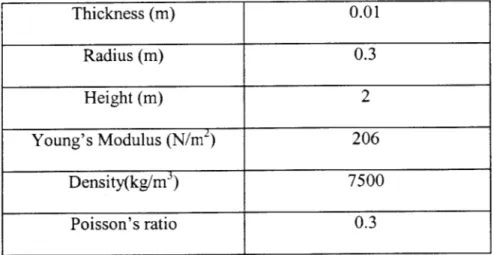
To compare the FE code with the analytical modeling, a simply supported cylinder with material properties and geometry as described in Table 3.1 was used for simulation by both approaches. 2 elements of length Im each were used to represent the cylinder, thus resulting in 8 degrees of freedom after 2 had been removed from each ends due to constraints of boundary conditions.

Table 3-1 Material properties and geometry of a simply supported natural frequencies

cylinder for comparing

The natural frequencies for the transverse vibration were plotted and compared as shown in Fig. 3.2 for both the analytical and FE model. The natural frequencies were not plotted for n values less than 3 for the FE model as the FE model was not able to produce eigenvalues corresponding to distinct mode shapes that represent resonance of transverse vibration. Moreover, it was also observed that the FE model agrees very well with the analytical model with slight discrepancies at lower order modes n = 3 and 4. This shows that the FE model generated from 2-D elements may not be able to represent the cylindrical shell for lower order modes as well as higher order modes.

Thickness (m) 0.01 Radius (m) 0.3 Height (in) 2 Young's Modulus (N/m2) 206 Density(kg/m3) 7500 Poisson's ratio 0.3