HAL Id: tel-03021210
https://tel.archives-ouvertes.fr/tel-03021210
Submitted on 24 Nov 2020
HAL is a multi-disciplinary open access
archive for the deposit and dissemination of sci-entific research documents, whether they are pub-lished or not. The documents may come from teaching and research institutions in France or abroad, or from public or private research centers.
L’archive ouverte pluridisciplinaire HAL, est destinée au dépôt et à la diffusion de documents scientifiques de niveau recherche, publiés ou non, émanant des établissements d’enseignement et de recherche français ou étrangers, des laboratoires publics ou privés.
To cite this version:
Sebastian Arturo Ceballo Charpentier. Causal manipulations of auditory perception and learning strategies in the mouse auditory cortex. Neurobiology. Sorbonne Université, 2019. English. �NNT : 2019SORUS058�. �tel-03021210�
Sorbonne Université
École Doctorale Cerveau-Cognition-Comportement (ED3C)
Paris-Saclay Institute of Neuroscience (NeuroPSI)
Doctoral Thesis
Causal manipulations of auditory perception
andlearning strategies in the mouse auditory cortex
Sebastian Arturo Ceballo Charpentier
Supervisor:
Dr. Brice Bathellier
Thesis committee members:
Dr. Maria Neimark Geffen.
Examiner
University of Pennsylvania. Philadelphia. United States of America
Dr. Kerry Walker.
Examiner
University of Oxford. Oxford. United Kingdom
Dr. Philippe Faure.
President of the committee
Institut de Biologie Paris-Seine (IBPS). Paris. France
Dr. Brice Bathellier.
Thesis director
Paris-Saclay Institute of Neuroscience (NeuroPSI). Gif sur Yvette, France
External invited expert:
Dr. Jean-François Leger
‘You have to die a few times
before you can really live’
i
Abstract
Through our senses, the brain receives an enormous amount of information. This information needs to be filtered and refined in order to extract the most salient features that will help us to guide our behavior. In this process, the brain encodes the environment into an internal ‘perceptual world’ in correspondence with our changing needs. An important advantage also is the ability to create new associations about external cues and their behaviorally relevant outcomes. This gives the possibility to generate predictions and respond precisely to various events in a challenging and always changing environment. Thus, previous experiences will shape our sensation and determine the responses to perceptual-based decisions.
The study of sensory perception is complicated as we cannot have direct access to well-isolated internal sensory representations. These representations need to be inferred from animal behavior in response to well characterized sensory stimuli. In this context, the study of animal learning and its contingencies are key elements for the study of sensory representations, as different learning strategies or learning rules can lead to different behavioral outcomes. How the brain actually extracts and generates these different perceptual features and wires them to behavior remains the two major questions in modern neuroscience. To answer these questions, novel neural engineering approaches are now employed to map, model and finally generate, artificial sensory perception with its learned or innate associated behavioral outcome.
In this work, we have used a combination of different modern technologies together with computational modeling to give important hints about the type of computations that auditory cortex performs under simple and more complex sound discrimination tasks. We have also explored the learning strategies that mice can adopt under a sound-basedperceptual discrimination task. More concretely, using a Go/noGo discrimination task combined with optogeneticsto silence auditory cortex during ongoing behavior in mice, we have established the dispensable role of auditory cortex for simple frequency discriminations,butalso its necessary role to solve a more challenging task. Specifically, we showed that for mice trained to discriminate between a frequency-modulated sound and a pure tone withboth startingat the same frequency,auditory cortex wasnecessary as discrimination was fully impaired during
ii
the optogenetic manipulations. By the combination of different mapping techniques and light-sculpted optogenetics to activate precisely defined tonotopic fields in auditory cortex, we couldelucidate the strategy that mice use to solve the task, revealing a delayed frequency discrimination mechanism.In parallel, observations about learning speed and sound-triggered activity in auditory cortex led us to study their interactions and causally test the role of cortical recruitment in associative learning. Using modern optogenetics, we reproduced a well-known cue interaction phenomenon that has been observed in different learning paradigms, the overshadowing effect. These precise cortical manipulations demonstratedthat neuronal recruitment can be thoughtof as the neurophysiological correlate of saliency. The description of this relationship confirms implicit assumptions of mainstream associative learning theories. Altogether these results push forward our comprehension of the learning rules governing sensory-based associations in the brain.Finally and more broadly, this work provides insight into the integrationof modern optical techniques into sensory rehabilitation approaches in order to improve sensory feature mapping and sensory discrimination e.g. hearing-impaired patients.
iii
List of content
Abstract ... i
List of figures ...vii
List of tables ...x
List of equations ...x
List of abbreviations... i
1. General introduction ... 1
1.1. The cerebral cortex ... 1
1.1.1. Columnar organization ... 1
1.1.2. Senses and their organization in the cortex... 2
1.1.3 Perspective ... 8
1.2. The auditory system ... 9
1.2.1. Overview ... 9
1.2.2. Lower auditory structures ... 9
1.2.3. The auditory cortex ... 18
1.2.4. Sensory perception and behavior ... 31
1.3. Learning and modeling animal behavior ... 33
1.3.1. Classical and operant conditioning ... 33
1.3.2. Discrimination and generalization ... 35
1.3.3. Learning from predictions ... 40
1.3.4. Rescorla-Wagner Model ... 42
1.3.5. Attention based models ... 44
1.3.6. Adaptive network models ... 50
iv
1.3.8. Neuronal basis of associative learning ... 55
1.4. To record, decode and manipulate neuronal representations ... 58
1.4.1. Linking two disciplines ... 58
1.4.2. Role of auditory cortex in the discriminations of sounds ... 60
1.4.3. Acute manipulations of cortical representations ... 62
2. Results: Section I ... 71
Targeted cortical manipulation of auditory perception ... 72
2.1. Abstract ... 72
2.2. Introduction ... 73
2.3. Results ... 74
2.3.1. Requirement of auditory cortex depends on sound discrimination complexity... 74
2.3.2. Information from auditory cortex can drive slow discriminative choices ... 76
2.3.3. Focal auditory cortex stimulations bias decisions in the complex discrimination ... 81
2.3.4. Tonotopic location of effective focal stimulations matches frequency cues used for discrimination ... 83
2.4. Discussion ... 87
2.5. Material and methods ... 91
2.5.1. Experimental model and subject details ... 91
2.5.2. Behavioral experiments ... 91
2.5.3. Behavior analysis. ... 92
2.5.4. Cranial window implantation. ... 92
2.5.5. Optogenetics inactivation of AC during behavior... 93
2.5.6. Patterned optogenetics during ongoing behavior. ... 93
2.5.7. In vivo electrophysiology. ... 95
v
2.5.9. Auditory cortex lesions and immunohistochemistry. ... 97
2.5.10. Intrinsic imaging and alignment of tonotopic maps across animals. ... 97
2.5.11. Two-photon calcium imaging. ... 98
2.5.12. Quantification and statistical analysis ... 99
2.5.13. Data and software availability ... 100
2.6. Acknowledgements ... 100
2.7. Author contributions ... 100
2.8. Supplementary figures ... 101
3. Results: Section II ... 109
Cortical recruitment determines learning dynamics and strategy ... 110
3.1. Abstract ... 110
3.2. Introduction ... 111
3.3. Results ... 112
3.3.1. Sounds with identical levels can recruit different activity levels ... 112
3.3.2. Cortical recruitment influences learning speed... 116
3.3.3. A reinforcement learning model reproduces recruitment effects ... 118
3.3.4. Learning speed effects depend on initial synaptic strengths ... 122
3.3.5. Recruitment determines learning strategy ... 124
3.4. Discussion ... 128
3.5. Materials and methods ... 131
3.5.1. Animals ... 131
3.5.2. Two-photon calcium imaging in awake mice ... 131
3.5.3. Data analysis ... 132
3.5.4. Patterned optogenetics and intrinsic imaging ... 132
vi
3.5.6. Go/NoGo discrimination behavior ... 134
3.5.7. Reinforcement learning model. ... 135
3.5.8. Statistical tests ... 136
3.5.9. Data and software availability ... 137
3.6. Acknowledgements ... 137
3.7. Author contributions ... 137
3.8. Supplementary figures ... 138
4. General discussion ... 144
4.1. Learning and remodeling of auditory cortex ... 144
4.2. Frequency discrimination without AC ... 146
4.3. Frequency modulated sound vs pure tone ... 148
4.4. Optogenetics to study sensory perception ... 152
4.5. General observations ... 154
4.6. Considerations about the auditory neural code ... 156
4.7. Therapeutic strategies using optogenetics ... 158
4.8. Towards a complete and inclusive learning model... 159
4.9. Concluding remarks... 161
vii
List of figures
Figure 1-1. Human and rodent body representations in the primary somatosensory cortex. ... 4
Figure 1-2. Orientation maps from the visual cortex of the cat. ... 5
Figure 1-3. Taste representations in the cortex of humans and mice. ... 6
Figure 1-4. Single odor representations in the olfactory bulb. ... 8
Figure 1-5. Schematic view of the auditory system. ... 10
Figure 1-6. Structures of the middle ear. ... 11
Figure 1-7. The cochlea and the basilar membrane. ... 13
Figure 1-8. Brainstem auditory sound localization circuits. ... 14
Figure 1-9. Schematic representation of auditory thalamus projections to AC. ... 17
Figure 1-10. Schematic representation of AC in some of the most studied mammals. ... 19
Figure 1-11. Schematic representation of the mouse AC. ... 21
Figure 1-12. Schematic tonotopy of superficial layers in the mouse AI. ... 23
Figure 1-13. Radial neuronal migration in the developing brain. ... 24
Figure 1-14. Sound onset latency and recording depth for multi-units in AI. ... 25
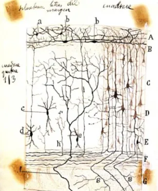
Figure 1-15. Drawing by Santiago Ramón y Cajal of the cerebral cortex... 28
Figure 1-16. Principal excitatory neurons in layer IV of the neocortex. ... 29
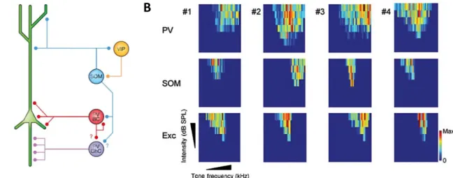
Figure 1-17. Schematic representation of neocortical circuits and their responses to sounds. ... 31
Figure 1-18.Pavlov’s conditioning and Thorndike’s puzzle box experiments. ... 34
Figure 1-19. Performance of one animal in a sound discrimination task. ... 36
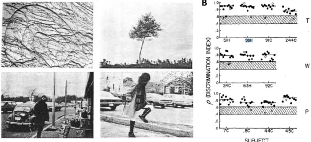
Figure 1-20. Pictures used to trained different groups of pigeons and generalization results. ... 37
Figure 1-21. Generalization experiments using images or sounds... 39
Figure 1-22. Patterns used in an Intra-Extra dimensional binding experiment ... 46
Figure 1-23. Diagram of a classic adaptive network model. ... 50
Figure 1-24. Learning curves of pigeons trained in a classicalpavlovian conditioningtask... 53
Figure 1-25. Sketch of the multiplicative reinforcement model for associative learning. ... 54
Figure 1-26. Individual and averaged learning curves for an associative learning task in mice. ... 55
Figure 1-27. Dopamine dynamics of DA neurons during a conditioning task. ... 56
viii
Figure 1-29. Different opsins allow the bidirectional control of neuronal activity. ... 64
Figure 1-30. Focal silencing strategy in awake animals. ... 66
Figure 1-31. Cortical activation of superficial layers in S1 of freely moving mice and cell quantification. . 67
Figure 1-32. 2AFC task in rats and frequency detection bias. ... 68
Figure 1-33. Perceptual decision bias in monkeys by micro-stimulation in AL. ... 69
Figure 2-1. Discriminating a FMs from a PT is harderthan two PTs. ... 75
Figure 2-2. Cortical requirement for sound discrimination depends on discrimination complexity. ... 77
Figure 2-3. 2D-light pattern triggers focal activity in auditory cortex. ... 78
Figure 2-4. Mice can discriminate two artificial activity patterns in AC. ... 80
Figure 2-5. Focal optogenetic AC activation can bias behavioral decisions. ... 82
Figure 2-6.AC neurons coding for intermediate frequencies distinguish sounds from the difficult task.... 84
Figure 2-7.Mice use intermediate frequencies as a cue to discriminate between FM sound and low frequency PT. ... 86
Figure 2-8. PV interneuron activation strongly perturbs AC responsesto sounds. ... 101
Figure 2-9. Irreversible lesions covered the full extent of auditory cortex. ... 102
Figure 2-10. Discriminated artificial optogenetic stimuli were located insimilar tonotopic locations across mice... 103
Figure 2-11. Reaction time for detection of a single focal cortical stimulus is similar to discrimination time for choosing between two focal cortical stimuli. ... 104
Figure 2-12. Tonotopic maps from intrinsic and two-photon calcium imaging are similar. ... 107
Figure 2-13. Stability of AC sound representations despite context dependent modulations. ... 108
Figure 3-1. Spectro-temporal differences in complex sounds do not affect near-threshold detectability ... 113
Figure 3-2. Spectro-temporal differences impact on cortical recruitment. ... 115
Figure 3-3. Cortical recruitment differences impacts learning phase duration. ... 119
Figure 3-4. A multiplicative reinforcement learning model reproduces modulations of learning speed by neuronal recruitment ... 121
Figure 3-5. The effects of neuronal recruitment in the model are explained by the differential adjustment of synaptic weights during learning... 124
Figure 3-6. Discrimination training of multi-spot optogenetic patterns reveals a choice of learning strategy depending on the level of cortical recruitment. ... 127
ix
Figure 3-7. Cortical recruitment differences are robust across mice and experiments ... 138
Figure 3-8. Impact of cortical recruitment on learning and delay phase durations. ... 139
Figure 3-9.The impact of neuronal recruitment on learning speed depends on the initial strengths of synaptic connections in the model ... 140
Figure 3-10. The effects of neuronal recruitment in the model do not crucially depend on the magnitude of recruitment differences. ... 141
Figure 3-11. Cortical responses to patterned optogenetic stimulations. ... 142
Figure 4-1. Error type for mice during AC silencing. ... 150
x
List of tables
Table 1. Summary of a simple training strategy of blocking. ... 41
Table 2. Summary of a training experiment of blocking using a discrimination paradigm ... 41
List of equations
Equation 1. R-W’s model of associative learning ... 42Equation 2. Blocking results explained using R-W’s terms ... 43
Equation 3. Mackintosh’s model of associative learning ... 46
Equation 4. Calculation of associative power according to Pearce and Hall’s model... 48
Equation 5. Pearce and Hall’s model of associative learning ... 48
i
List of abbreviations
Affaires
2AFC: Two alternative forced choice 161 AAF: Anterior auditory field 19
AC: Auditory cortex 9
AChE: Acetylcholinesterase 18 AI: Primary auditory cortex 10 ChR: Channelrhodopsin 63 CN: Cochlear nucleus 10 CNIC: Central nucleus of the inferior culliculus CO: Cytocrome oxidase 18 CS: Conditioned Stimulus 33 DCIC: Dorsal cortex of the inferior culliculus 15 IC: Inferior colliculus 14 ILDs: Interaural level differences 14 ITDs: Interaural time differences 14 LCIC: Lateral cortex of the inferior culliculus 15 LSO: Lateral superior olive 14 MGB: Medial geniculate nucleus 10 MGd: dorsal nucleus of medial geniculate body MGm: medial nucleus of medial geniculate body MGv: ventral nucleus of medial geniculate body MSO: Medial superior olive 14 nBIC: Branchium of the inferior culliculus 15 NS: Neutral Stimulus 33
PV: Parvalbumin 18
S1: Primary somatosensory cortex 3 SC: Superior culliculus 15 SOC: Superior olivary complex 10
UCR: Unconditionned Response 33 UCS: Unconditioned Stimulus 33 V1: Primary Visual Cortex 5
1
1. General introduction
1.1. The cerebral cortex
The link between the brain, and sensory perception becomes most dramatically evident in cases of loss or disturbance of perceptual functions after some form of brain damage (Sacks, 1985). From the periphery, the information finally arrives to the cerebral cortex into hierarchically organized sensory areas, where it is processed and sent to different ‘higher’ areas in the brain. In mammals, the cerebral cortex has a central role indifferent cognitive processes, analysis, integration and sensory perception, as also in planning of goal directed behavior, learning and memory retrieval. Composed of the allocortex (containing the archicortex or the hippocampal region and the paleocortex or olfactory cortex) and the iso or neocortex, this structure is considered the evolutionarily youngest brain region (Gao et al., 2013). Structural as well as functional principles within cortical circuits, especially in primary sensory areas, display a high degree of conservation across different species, even in the lissencephalic rodent brain. These conserved characteristics allow experimental studies in the laboratory using different animal models and the post-hoc extension to understand the general organization and principles of the human brain (Schreiner et al., 2000).
1.1.1.
Columnar organization
Early observations of the sensory systems in the brain by Santiago Ramón y Cajal and one of his disciples Rafael Lorente de Nó, noted the presence of vertically arranged and highly connected cells (de Castro and Merchán, 2017; Larriva-Sahd, 2014). Years later Vernon Mountcastle, using electrophysiological recordings in the somatosensory and motor cortex of cats and monkeys, described how these columnar structures responded to the same type of mechanical stimulus (Mountcastle, 1957; Mountcastle and Powell, 1959). The preceding efforts of Hubel and Wiesel in the 1960s, studying the primary visual cortex of cats, led to the discovery of ‘orientation columns’ and ‘ocular dominance columns’, corroborating previous observations and theories about the functional columnar organization of the principal sensory systems in the neocortex (Hubel and Wiesel, 1959; Hubel and Wiesel, 1962), which have been later
2
validated by many different techniques (Ohki et al., 2006). From these foundational studies, similar structural principles were observed studying other sensory modalities as for example, the frequency tuning in auditory cortex of different species including humans (Goldstein et al., 1970; Winer, 2011). Following with this idea, it has been largely observed and described that in each sensory domain, neurons tend to be preferentially clustered in groups that share similar input features and response properties (Andermann and Moore, 2006; Schubert et al., 2007; Ko et al., 2011; Issa et al., 2014 ; Deneux et al., 2016 ; Issa et al., 2017; Bimbard et al., 2018). Recently proposed, this characteristic of neocortical circuitswould emerge during development, where cells that belong to the same progenitor are preferentially connected creating local connectivity patterns(Kandler et al., 2009). Later, through sensory experience, these circuits would be refined by Hebbian plasticity mechanisms (Peinado et al., 1993; Gao et al., 2013) and different connectivity rules at macro and micro-scales (Barkat et al., 2011; Vasquez-Lopez et al., 2017; Hayashi et al., 2018; Nishiyama et al., 2019).
1.1.2. Senses and their organization in the cortex
An important characteristic of the previously described neocortical columnar organization, is that often reflects some of the corresponding sensory topographic representation in the periphery (Douglas and Martin, 2007; Larriva-Sahd, 2014; de Castro and Merchán, 2017). Neurons in the peripheral nervous system are fundamental units of information processing, capturing and translating changes in our environment into a readable code for the brain. The five most commonly described senses, olfaction, vision, gustation, touch and hearing, emerge from specialized sensory receptors neurons that can be classified on the basis of their structure, position and functionality in relation to the stimuli they sense. Regarding structural characteristics they are clustered in three groups; neurons with free nerve endings sensing directly the stimuli, neurons with encapsulated ending of connective tissue and specialized receptor neurons with special components that translate the stimuli into electrical signals (Purves, 2004). Classified also by their position, they can be grouped as an exteroreceptor; if it is located near the stimulus in the environment, interoreceptor; if it senses internal organs or internal variables as blood pressure, or propioreceptor; located near a muscle or an area in the body that receives motion signals (Purves, 2004). Classified by their functionality, sensory receptors can be chemoreceptors that translate chemical sensation, osmoreceptors that respond to solute concentrations, nociceptor that detect the presence of certain molecules, mechanoreceptors that are in charge of physical stimuli such as variations
3
in pressure and thermoreceptors which are sensitive to temperature (Purves, 2004). Each sensory modality is then equipped with one or more of these different types of receptors,in order to transduce different type of signals. From the periphery, the information flows through the axons of interconnected neurons to finally reach the brain (Hackett, 2011). Besides the important number of relay and processing stations from periphery to primary sensory areas in the neocortex(Krubitzer, 1995), important sensory features can be foundin the cortical surface in form of representational maps. In the following sections, before a complete description of the auditory system, I will briefly describe some of these sensory representations in the cortex. Sensory representations those are accessible using different type of techniques but which precise role for sensory perception has not been yet fully addressed.
Somatosensation
The somatosensory system is composed of two major components: one in charge of the detection of mechanical stimuli and another for the detection of pain and temperature. Somatosensation is in this way related to several sub-modalities such as light touch, vibration and pressure that via a diverse set of neural receptors, mainly mechanoreceptors located in the skin and hair follicles, convey the information in a topographic manner through several ascending pathways to the spinal cord, brainstem, and ventral posterior complex in the thalamus to finally reach the primary somatosensory cortex (S1). In humans, S1 is located in the postcentral gyrus of the parietal lobe (Brodmann’s areas 3a, 3b, 1 and 2) and each of these zones contains an entire somatotopic representation of the body (Figure 1-1A). In each of these parallel somatotopic maps, neurons encode specific to certain features of skin stimulation such as texture, shape or movement direction(Purves, 2004). In rodents, the body representation is largely biased towards the topographical representation of the whisker pad, containing the classic ‘barrels’, where each of them is composed of neurons responding to principally one specific whisker of the whisker pad (Benison et al., 2007) (Figure 1-1B-C). Also recent observations in rodent S1 have described that neurons within a single barrel column appear to be spatially clustered forming a map of orientation selectivity within single barrel columns(Andermann and Moore, 2006; Kremer et al., 2011).
4
Figure 1-1. Human and rodent body representations in the primary somatosensory cortex.
(A) Diagram showing the location of the human primary somatosensory cortex (S1) in the brain and schematic of the body representation in a coronal view of S1. Also a classic representational quantification of the area dedicated to each part of the body (homunculus) made in the 1930s but still generally valid. Adapted from Purves (2004). (B) Same representation as A but for a rat. The Rattunculusshows graphically the area dedicated to each part of the rat’s body in S1 and S2 in the brain. From Benison and colleagues (2007) (C) Barrel cortex in a mouse stained with cytochrome oxidase to reveal the ‘barrels’ in dark grey in S1. Each barrel is labeled with the stander nomenclature representing each whisker on the mouse snout. From Schubert and colleagues (2007).
Vision
The visual system begins with one of the most advanced sensory organs, the eye. The eye, along with its lens and muscles, focuses and modulates the amount of light that is received at back part of the globus ocularis, where the retina is found. In the retina, there are specialized receptor neurons that contain a light-sensitive photo pigment, called photoreceptors. These neurons are dedicated then to the detection of photons and their transformation into electrical signals. The extremely well organized architecture of the retina, transforms already the information at this stage, emphasizing some aspects of the visual field, that will be sent through the optic nerve and optic track to several brain structures such as the
5
pretectum (involved in pupillary light reflex), the suprachiasmatic nucleus of the hypothalamus (involved in the day/night cycle), the superior colliculus (involved in the coordination of head and eye movements) and the thalamus (Purves, 2004). Visual information arrives firstto the dorsal lateral geniculate nucleus (LGN) in the thalamus, from where is sent mainly to the primary visual cortex (V1). The spatial organization of the photoreceptors in the retina is maintained through the whole visual pathways, creating organized visual representations of the space or retinotopy. Most of the neurons in the visual pathway receive information from both eyes but as a general rule, the left half of the visual field is represented in the right half of the brain, and vice versa (Purves, 2004). In humans, V1 is located in the calcarine fissure in the occipital lobe (Brodmann’s area 17), where V1 neurons are mainly responsive to the orientation of edges in a simple or in a more complex way, where approximately all edge orientations are equally represented in the form of orientation columns (Hubel and Wiesel, 1962;Ohki et al., 2006) (Figure 1-2). The description of visual cortical neuron receptive fields and their organization is an enormous field of active research, which have showed that basic spatial organization principles are relatively well conserved across species (Krubitzer, 1995). However, recent observations in rodents mitigate this idea whereas contrary to cats and monkeys, visual stimulus orientation in the rodent primary visual cortex would be represented in a ‘salt and pepper’ organization, showing substantial heterogeneity in the tuning properties of neighboring neurons (Bachatene et al., 2016).
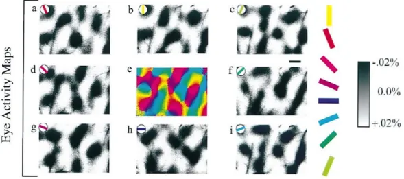
Figure 1-2. Orientation maps from the visual cortex of the cat.
Orientation preference maps obtained with optical imaging of intrinsic signals from the visual cortex of an anesthetized cat. Dark areas correspond to regions in the cortex that are active during the monocular presentation of a grating at the orientation indicated in the upper left
6
part of each image (all panels but e). In the center, the summed imaged of all orientation preference map color coded to each direction. Scale bar: 500 mm. Adapted from Crair and colleagues (1997).
Gustation
Gustation is one of the chemical senses and is in charge of the detection of taste. Gustatory receptor neurons in the taste buds or papillae, mainly located on the tongue and upper digestive track, detect chemicals (sweet, bitter and umami) and ions (salty and sour). Taste cells are then innervated by branches of the facial (VII), glossopharyngeal (IX) and vagal (X) nerves which contact the gustatory nucleus of the solitary tract in the medulla (Purves, 2004). The rostral part of this nucleus sends projections to the ventral posterior medial nucleus in the thalamus, which in turn sends projections to the anterior insula in temporal lobe, the operculum of the frontal lobe and also to a second group of neurons in the caudolateral orbitofrontal cortex, where neurons are involved in satiety and motivation to eat (Pritchard et al., 2008). Neurons along the taste pathway are particularly responsive for one taste and the information flows in a sort of topographic map to the brain, creating separate taste representations in the cortex (Chen et al., 2011; Prinster et al., 2017).
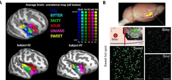
Figure 1-3. Taste representations in the cortex of humans and mice.
(A) Functional magnetic resonance imaging (fMRI) responses to the standardized five basic tastes together with a cortical surface representation of the human right insular cortex in two different subjects and average image in a pilot study. Adapted from Prinster et al., (2017). (B) Two photon calcium imaging in the mouse insular cortex. On top image of the brain with the approximate location of the recording site in the primary taste cortex (yellow). On bottom,
7
neurons are represented with small circles and high neuronal responses to different tastants in a single trial color coded for the same recording site, depending on the stimulus applied to the animal’s tongue. Adapted from Chen and colleagues (2011).
Olfaction
Olfaction, the other chemical sense, is in charge of the detection of small molecules called odorants. Olfactory receptors neurons are located on a relatively small portion of tissue in the nose. In close contact with the different odorants dissolved in the mucus, receptor cells detect and transduce these signals through the olfactory tract. The precise information arrives to a single glomerulus, where then is split to different sensory areas of the brain(Johnson and Leon, 2000; Rubin and Katz, 1999; Stewart et al., 1979). Afferent projections from the olfactory bulb mainly reach the piriform cortex, in humans located in the temporal lobe. This sensory system is really unique as it is the only one not containing a thalamic relay.Also, the main area dedicated to it in the cortex is not six-layered, but only thee-layered cortex. Another difference of this system is the poor feature representation in the olfactory bulb and pyriform cortex, as no map of odorant features has been described yet (Purves, 2004; Choi et al., 2011). Despite the lack of fine representations, large-scale odor responses in the olfactory bulb glomeruli can be used to predict the identity of odors in rats (Linster et al., 2001) (Figure 1-4A-B). Olfactory receptor neurons vary greatly in the diversity of G-coupled protein receptors at their cell surface (more than 400 in human and close to 1200 in rodents) (Purves, 2004). These particularities make odor perception vary a lot depending on the molecular structure, concentration and timing of exposition of the different odorants in the air, as also the fact that the constitution of the most common odor’s perception is in fact the result of a complex mixture of odorant molecules.
8
Figure 1-4. Single odor representations in the olfactory bulb.
(A) Surface of the olfactory bulb and optical imaging of intrinsic signals in response to different odorants in the rat olfactory bulb. Dark areas represent neuronal activations in presence of each odor presentation in the same area. Scale bar 250 µm. Adapted from Rubin and Katz (1999). (B) Contour of the different areas in the olfactory bulb of a rat and average deoxyglucose charts showing the spatial distribution of [14C]2-deoxyglucose uptake evoked by different odorant enantiomers. Adapted from Johnson and Leon (2000).
1.1.3 Perspective
The columnar organization of sensory features in the mammalian neocortex revised here corresponds to a fundamental principle observed in almost all species studied. Yet one of the major goals of sensory neuroscience is try to link these cortical representations with the precise sensory percepts and their role in for example, learning and memory recall. Modern neurophysiological techniques make possible today formulate and test these type of causal hypothesis. After a comprehensive description of the auditory system and associative learning theory, several attempts on this venue willbe described, as they constitute the background and supportof the work presented here.
9
1.2. The auditory system
1.2.1. Overview
Most hearing research today focuses on the study of both, normal and pathological aspects of hearing comprehending different animal models. Comparative hearing research has been able to determine some of the fundamental principles shared across species for the main structures of the auditory system, their physiological functions and their role for different hearing abilities, often with a successful translation to the human auditory system. This system depends on highly evolved and complex structures as well as external physiological processes. The ear, first auditory relay station, is responsible for the detection and decomposition of sounds. Sound is the oscillation of air molecules in the form of three dimensional waves. As any wave, sound waves contain three major features; phase, amplitude or loudness and frequency or pitch. Most natural sounds are composed of complex waveforms of sinusoidal waves varying in amplitude, frequency and phase. The hearing bandwidth (the audible range) has been tested in more than 60 mammalian species. Varying only in some extreme cases, it shares some important similarities and generalizations, such as the minimum sound detection thresholds (Schreiner et al., 2000; Vater and Kössl, 2011). These conserved fundamental hearing capabilities reflect the coevolved adaptations of the middle and inner ear across most mammalian species (Basch et al., 2016). In general, all mammals analyze and decompose the sound into its constituent frequency components with different degrees of resolution (Mann and Kelley, 2011). The ear then is a highly specialized biological Fourier analyzer of sound waves, followed by an extremely well organized hierarchical routing system that allows the transformation and segregation of sound into a precise neural code.
1.2.2. Lower auditory structures
The first stage of sound transformation occurs in the external and middle ear, where air vibrations are amplified and transmitted to the cochlea in the inner ear. There, frequency, amplitude and phase are transduced by hair cells and then transmitted to the central nervous system by the auditory nerve. One key feature of the auditory system is the topographic organization or tonotopy of its projections from the cochlea to the auditory cortex (AC) in the brain, in what is called the lemniscal pathway. From the
10
cochlear nucleus (CN), the auditory information flows in parallel tonotopic streams, that reach first the superior olivary complex (SOC), where the information of the two ears first interacts allowing the localization of sound in space. Following the pathway, the next stage is the inferior colliculus (IC) in the midbrain, where auditory information is integrated and interacts with the motor system (Casseday and Covey, 1996; Xiong et al., 2015). The IC projects to the medial geniculate nucleus (MGB) in the thalamus, which in turn projects to the primary auditory cortex (AI) (Figure 1-5). Here the information is routed to different secondary auditory areas in the brain and feedback to the thalamus and the IC in a dynamic manner. The auditory pathway is very complex as it counts on many feedforward and feedback projections and only an overview of the main processing stations and their connections is provided.
Figure 1-5. Schematic view of the auditory system.
All nuclei of the lemniscal auditory pathway are tonotopically organized. Cochlear nucleus (CN), superior olivary complex (SOC), inferior colliculus (IC), and medial geniculate nucleus (MGN).Primary (belt), secondary (belt) and tertiary (parabelt) auditory cortex in the human brain are located in the superior part of the temporal lobe. From Saenz and Langers (2014).
11
Periphery
External EarThe external ear corresponds to the visible part of the auditory system and comprises the pinna, concha, ear canal and eardrum or tympanic membrane. Sound waves are captured in the pinna, then enter the ear canal and push the tympanic membrane which will vibrate according to the sound waves, transmitting them to the middle ear. In humans, this region particularly enhances the detection of sound around frequencies close to human speech, as this perceptual system is thoughtto have evolved to encode environmental stimuli in the most efficient way (Gervain and Geffen, 2019).
Middle Ear
The function of the middle ear is to act as interface between the mechanical boundaries between the air-filled spaces of the external ear with the liquid-air-filled spaces of the cochlea. This structure is composed of three small bones (ossicles) called the malleus, incus and stapes. These bones form a sort of chain that match the distinct resistances encountered from the air to an aqueous fluid – perilymph and endolymph – in the inner ear. In simple terms, a wave traveling through the air is too weak to cross this air-water boundary and produce the same oscillations, so the energy or pressure of the sound wave needs to be concentrated in a small area. This transformation occurs thanks to the close contact of the malleus with the tympanic membrane, its anchorage with the incus which in turn moves the stapes, the final part of the chain that is in contact with the cochlear surface through the oval window. The correct sound transmission and transformation is also regulated by two muscles in the middle ear, regulating the stapedius reflex (also called the acoustic reflex), which is triggered by loud noises or self-generated vocalizations to reduce the amount of energy transmitted to the cochlea.
12
In the middle ear are located the auditory ossicles. These three small bones are in charge of the transformation of sound air waveforms, which impact the tympanic membrane, into oscillations in a liquid media inside the cochlea, through extremely precise movements of the oval window. Also are shown the cochlea and the vestibular system. From Nyberg and colleagues(2019).
Inner ear
Apart from the cochlea, in the inner ear is also located the vestibular system, responsible for the sense of balance by the continuous gathering of information concerning direction and acceleration of the head in the space. The cochlea is the most critical and important structure in the auditory system, which with its coiled architecture, is where the pressure waves are amplified, decomposed and transformed into electrical pulses. This structure is divided into three fluid-filled chambers (the scale vestibule, scala mediaand the scale tympani) separated by two membranes, the Reissner’s membrane or tectorial and the basilar membrane. The basilar membrane is the most important for audition, as it lies over the Organ of Corti (see later), and covers the entire length of the cochlea, changing its thickness from narrow and stiff in the basal end (near the oval and round windows) to wider and more flexible in the apical end. The movement applied on the oval window, propagates through this membrane and also through the cochlear fluids from the base to the apex, depending on its frequency. Low frequencies will cause vibrations mostly at the apex of the basilar membrane and increasing frequencies will shift the maximal vibration toward the basal end. This means that each location of the basilar membrane will have a ‘best’ frequency, precisely translated to the Organ of Corti. This last structure contains the inner hair cells and outer hair cells, the mechanoreceptor neurons of the auditory system. The movement generated on the basilar membrane moves the cilia on inner hair cells, opening cation-selective channels near the tip, which leads to the entry of K+ ions into the hair cell. The increase in intracellular K+ results in the depolarization of the cell and, due to the entry of Ca2+ through voltage-gated Ca2+ channels in the soma, the release of neurotransmitters to the synaptic contacts with spiral ganglion neurons. Together, the axons of these neurons form the auditory branch of the vestibulocochlear or VIIIth cranial nerve. This process is non-linearly amplified, in a poorly understood manner, by outer hair cells depending on the frequency range of stimulation. In this way, each cycle of the sound wave is reflected by a sinusoidal change in the membrane voltage, which is extremely precise for the low frequency sounds (phase locked) but less precise or sensitive for high frequency ones, due to the continuous depolarization of the cell whose magnitude reflects then the amplitude of the stimulus (Cheatham, 1993). Extracellular
13
recordings of an auditory nerve fiber stimulated at different frequencies, have shown that spikes tend to occur near the crest of the sine wave (when the deflection of the stereocilia of the hair cells is maximal) but not with clockwork precision (Schnupp et al., 2011). This is due to nerve fibers changing their firing rates from roughly Poisson distributed intervals to a lessregular phase-locked mode. This effect depends on the frequency of stimulation, as they can skip some cycles or spikes can occur not on the crest of the wave (Schnupp et al., 2011). In summary, as single hair cells respond to a specific narrow frequency band, the collection of hair cell response features creates the tonotopy observed along the whole auditory pathway present in almost all mammals studied (Schnupp et al., 2011).
Figure 1-7. The cochlea and the basilar membrane.
(A) Schematic structure of the cochlea that shows the basilar and tectorial membrane, as well as the location and organization of the different cell types that generate the mechanostransduction of oscillations into electrical activity by the inner hair cells. From Kapuria and colleagues (2017)(B) Summary of the most important physical properties of thebasal-to-apical basilar membrane,as frequency tuning, thickness, cell type and their basic morphological characteristics.Adapted from Basch and col (2016).
Cochlear structure
14
Auditory nuclei
Cochlear nucleusThe auditory nerve fibers join the VIIIth cranial nerve after leaving the cochlea and project to the first relay station of the auditory system, the CN. As described before, each nerve fiber receives inputs from only one inner hair cell projecting to the ipsilateral CN in the brainstem, which is divided into two parts: the ventral part and the dorsal part. At this stage, terminals of the auditory nerve axons differ in density and type, innervating different populations of CN neurons with different properties. Neurons of the CN differ in their anatomical location, morphology and spectro-temporal response profiles but importantly the connections maintain thecochlear tonotopic organization. Neurons of the ventral part of the CN project ipsilaterally and contralaterally to the SOC and neurons from the dorsal part bypass the SOC and project directly to the nuclei of the lateral lemniscus on the contralateral side to then arrive at the IC, the first processing station of the midbrain.
Olivary complex
In this structure, the spatial position of the sound is encoded using either Interaural Time Differences (ITDs) for low frequencies (< 3 kHz) in the medial superior olive (MSO) or Interaural sound Intesity Differences (ILDs) for high frequency sounds (> 2 kHz) in the lateral superior olive (LSO) (Kandler et al., 2009) (Figure 1-8). Later, ascending fibers reach the contralateral nucleus of the lateral leminiscus which in turn projects toward the IC.
15
Tonotopic distribution of cochlear outputprojections that innervate the cochlear nucleus (CN). From the CN excitatory (green) and inhibitory (red) connections are detail with the lateral superior olive (LSO) and medial superior olive (MSO). Together these circuits make possible sound localization in space based on spike time differences. HF; High frequency sounds, LF; Low frequency sounds.Adapted from Kandler and colleagues(2009).
Inferior colliculus
Inputs from the brainstem nuclei converge along a fiber bundle known as the lateral lemniscus, which arrives in the IC together with commissural connections between left and right ICs. The IC is subdivided into several sub-regionscontaining one or severalsub-nuclei(C. Chen et al., 2018). Generally the IC is subdivided in core (ICc) and shelter (ICx) regions. ICc is compose of the central nucleus (CNIC) which receive most input from the lemniscal pathway arriving from the brainstem. The CNIC is then surrounded by the ICx, which is composed of the dorsal cortex at the top (DCIC), the external or lateral cortex (LCIC) and the nucleus of the branchium (nBIC) (Chen et al., 2018) (Figure 1-9). Together to the ascending projections from lower auditory stations that innervate the IC, there are an important amount of cortifugal projections arriving to ICx (Bajo et al., 2007; Winer et al., 1998), maybe participating in fine sound localization but their functions are not yet well stablish (Bajo et al., 2010) (Figure 1-9). The complicated pattern of innervations as the combination of binaural information in this structure generates complex neuronal responses, finding for example neurons responding to sound frequency, intensity, duration, as well as neurons able to encode sound localization due to ITD (Grothe et al., 2010; King et al., 1998). Other more refined features can also be found as for example, neurons in the IC of the barn owl, were they are not only tuned to specific horizontal regions in the physical spaces but also to preferred elevations (Grothe, 2018). Comparable maps have not yet been described in mammals, but other features can be found already at this stage such as frequency-modulation responsive neurons (Clopton and Winfield, 1974; Felsheim and Ostwald, 1996; Hage and Ehret, 2003; Rees and Møller, 1983). The CNIC is the structure tonotopically arranged, where neurons responding best to low frequencies are located near the dorsal surface and neurons responding progressively towards higher frequencies are located more ventrally (Barnstedt et al., 2015; Schnupp et al., 2011). ICx neurons send projections to the superior colliculus (SC) where auditory information interacts with head and reflexive eye movements to orientate them to unexpected sound sources(King et al., 1998). Most of the projections from the CNIC and DCIC arrive to the biggest processing and relay auditory nucleus in the thalamus, the MGB or as is simply known, the auditory thalamus(Figure 1-9).
16
Auditory thalamus
The MGB receives its inputs mainly from the IC but also direct projections from lower auditory nuclei. In general the MGB is described as an obligatory relay station for all of the ascending auditory projections. The MGB, as the IC, is subdivided into several sub-nuclei, most notably the ventral (MGv), dorsal (MGd) and medial nuclei (MGm) (Figure 1-9). The MGv is part of the lemniscal system,where neurons respond best to one particular frequency, and therefore the tonotopic organization is extremely well conserved. This area corresponds to the major thalamo-cortical relaywith approximately 85% of boutons arriving and clustered in layers III and IV in the cortex (Polley et al., 2007) (Figure 1-9). In parallel to this, the MGd is part of the non-lemniscal system as it receives less tonotopically organized projections from the CNIC (Lee, 2015). This area also sends projections to the granular layer of the cortex but with much more dispersion than MGv. MGm is also not well tonotopically organized receiving its inputs from all nuclei of the IC but also from other lower structures (Hackett, 2011). Neurons in the MGB are tuned not only to frequency, but to other complex features because of the convergence of spectrally and temporally separate auditory pathways (Malmierca et al., 2015). For example, neurons responding best to combinations of frequencies are first observed at this stage (Syka, 1997). Outputs from the MGB are many including dorsal striatum (Chen et al., 2019) and limbic structures such as the amygdala (Antunes and Moita, 2010), but in the vast majority of thalamic projections arrive to the primary and secondary auditory cortical areas (Hackett, 2011; Lee, 2015). Recent experiments indicate that the different subdivisions of the MGB in fact project to non-overlapping areas of the AC, where MGv projects to the core or primary auditory areas whereas theMGd sends its projections the belt or secondary and parabelt or terciary AC regions (Smith and Populin 2001) (Figure 1-9). Consequently, it is thought that in secondary and associative areas of the AC, the main input to layer IV would be projections from primary auditory cortical areas (Hackett, 2011). Mention that the MGB is only a relay station of auditory information to upcoming structures is mostly for schematics and representational reasons as it is well-known that corticofugal feedback projections from AC to the MGB outnumber largely the feedforward cortical projections of the MGB. Primary as well as secondary auditory areas project to all nuclei of the MGB meaning that information that is routed from the MGB to AC, is under constant transformation and strict control of these numerous corticothalamic feedback connections (Kimura et al., 2005; Winer et al., 2001; Winer and Lee, 2007).
17
Figure 1-9. Schematic representation of auditory thalamus projections to AC.
Feedforwardprojections from MGB to AC arrive to different auditory areas accordingly to the nuclei from they emerged. The ventral nucleus of the MGB projects mainly to AI whereas the dorsal and medialnucleus project towards secondary and tertiary auditory areas. Corticofugal projections reach all nuclei of MGB. Indicated with roman numbers are the neocortical layers from where connections arrive and exit the cortex.Black connections indicate ascending projections and red descending projections.Non-lemniscal areas arehighlighted in grey.FromMalmierca and colleagues (2015).
Secondary
18
1.2.3. The auditory cortex
The first evidence about the existence of a brain area dedicated specifically for the processing of sounds, came from the early experiments performed by David Ferrier in the 1870s (“Ferrier on the Functions of the Brain,” 1877). First, by direct galvanic stimulations and profound ablations of different areas of the brain in monkeys, he localized and described in much better detail, the motor cortex than his predecessors. Using similar techniques, he realized that precise stimulations in the superior temporal gyrus of monkeys generates a startle response and lesions in the temporal lobe generate severe deafness in the subjects without other apparent motor or cognitive deficiencies. After several decades of research, it is now known that only humans and macaques show some degree of hearing loss after removal or ablation of the AC, unlike smaller mammals such as ferrets, cats and dogs (Warren, 2005). Using diverse techniques, the AC has been precisely located and recognized as the last step in a long chain of hierarchically arranged stages of sound processing (Hackett, 2011). In humans and primates the AC, is located in the temporal lobe and is comprised of the superior temporal gyrus and Heschl’s gyrus. In ferrets, cats and dogs,it is located in the sylvian gyrus. Thanks to an extensive amount of research, the AC has been subdivided in a great number of sub-areas, where some of them show a clear and well organized tonotopy (Figure 1-10). Generally, there is evidence to suggest that in primates, there are at least three hierarchically arranged sub-areas within the AC, primary or ‘core’, secondary or ‘belt’ and associative or ‘parabelt’ (Winer, 2011). These different sub-areas, are delineated by their anatomical connectivity patterns, cytoarchitectonic characteristics, physiological criteria and different cell-biological markers (Hackett et al., 2001; Wallace et al., 1991). Primary areas are considered to be the main targets of the ascending lemniscal pathway and they are delimited by the extensive accumulation of granular-like neurons (mainly located in layer IV), short response latencies, strong expression of cytochrome oxidase (CO), acetylcholinesterase (AChE) and parvalbumin (PV), together with a strong myelination pattern. In contrast, secondary and more associative areas present large pyramidal neurons with longer response latencies, and a fractured tonotopic organization with diffuse myelination patterns and less metabolic activity (Polley et al., 2007; Kuśmierek and Rauschecker, 2009; Guo et al., 2012; Joachimsthaler et al., 2014).
In general, the core or primary auditory areas present two or three subdivisions, extensively characterized by tracer injections and extracellular recordings studies. In non-human primates these
19
subdivisions are the primary auditory cortex (AI), rostral area (R) and rostrotemporal area (RT), arranged from caudal to rostral (Figure 1-10). In other mammals, they are mainly defined as AI and anterior auditory field (AAF) (Hackett, 2011) (Figure 1-10). The homology of brain regions across species, particularly for these areas, is difficult as it shows an incredible specialization regarding the specific animal needs. For example in echolocating bats, there is a considerable number of areas specialized for the processing of echo delays and Doppler shifts, which obviously does not have a counterpart in the human or non-human primate brains (Grothe et al., 2010; Schnupp et al., 2011).
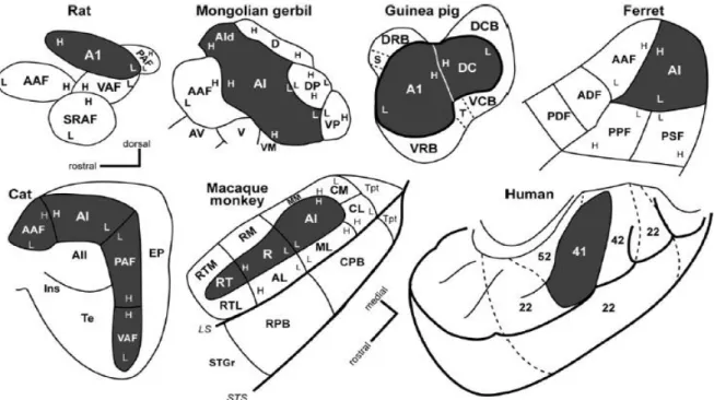
Figure 1-10. Schematic representation of AC in some of the most studied mammals.
Primary auditory areas are in darker color. Most of the secondary and tertiary areas described so far are also indicated. Low (L) and High (H) tonotopic fields are indicated in each panel. From Hackett and colleagues (2011).
The connectivity pattern in between the different sub-areas of the AC varies between species. While in carnivores, it is usually described that AI and AAF present comparable amounts of thalamic inputs, cortico-cortical connections and similar neurophysiological properties, the secondary auditory area or belt present very distinct connectivity patters (Figure 1-9). In non-human primates as well as in cats, it has been described that AI send direct projections to the secondary areas which in turn, send projections
20
back to AI and to the posterior ectosylvian region (comparable in some degree to the parabelt region in primates) (Fay and Popper, 1994).
Tonotopic organization
The first demonstrations of tonotopy were provided by recordings of evoked potentials in the exposed ectosylvian cortex of the cat, while stimulating isolated auditory nerve fibers from different regions of the cochlea (Woolsey and Walzl, 1942; Rose and Woolsey, 1949b). This structural organization was seriously doubted years later by several different groups arguing that responses from isolated units in AC were sparse (Davies et al., 1956; Evans and Whitfield, 1964; Gerstein and Kiang, 1964; Evans et al., 1965; Abeles and Goldstein, 1970) and highly modulated by several factors such as attention and anesthesia (Evans and Whitfield, 1964; Katsuki et al., 1959). Although some of these works argued in favor of the columnar organization of the AC, as they observed a clear macroscopic tonotopic organization after averaging the best or characteristic frequency from nearby isolated neurons, this started a long lasting dispute in the field (Goldstein and Abeles, 1975). The emergence of new technologies to precisely locate and record the activity of thousands of neurons at the same time and at different spatial resolutions (Denk et al., 1990; Grinvald et al., 1986), resurfaced the question about how good the tonotopic organization was maintained across neighboring neurons in the AC, especially in superficial layers. In humans there is evidence from MEG studies, recordings with implanted electrodes or functional imaging (fMRI) of at least one tonotopic gradient in the core region (Howard et al., 1996; Lütkenhöner and Steinsträter, 1998; Talavage et al., 2000). A mirror second tonotopic map has been described recently through high power fMRI, homologous to AI and R areas in the monkey’s brain (Formisano et al., 2003). For other mammals, large-scale tonotopic organization has been observed in great detail, using several low resolution optical techniques in the marmoset (Zeng et al., 2019), cat (Langner et al., 2009 ; Spitzer et al., 2001), ferrets (Nelken et al., 2004; Versnel et al., 2002), chinchilla (Harel et al., 2000; Harrison et al., 1998), gerbils (Schulze et al., 2002), rats (Bakin et al., 1996 ; Kalatsky et al., 2005) and mouse (Bathellier et al., 2012; Deneux et al., 2016; Horie et al., 2013; Issa et al., 2014; Issa et al., 2017; Kato et al., 2015; Kubota et al., 2008; Moczulska et al., 2013; Sawatari et al., 2011; Stiebler et al., 1997; Takahashi et al., 2006; Tsukano et al., 2015; Tsukano et al., 2016). Using microelectrode arrays/single electrodes or wide-field two photon calcium imaging recent studies have found the same macroscopic structural organization reported by low resolution optical techniques in the cat (Atencio and Schreiner,
21
2010), rat (Polley et al., 2007) and with high detail in the mouse cortex (Bao et al., 2001; Barkat et al., 2011; Guo et al., 2012; Hackett et al., 2011; Issa et al., 2014; Issa et al., 2017; Joachimsthaler et al., 2014; Stiebler, 1987; Yang et al., 2014; Zhang et al., 2005). Together these works removed all doubt about the large-scale tonotopic organization of the AC, underlining five subdivisions: two highly tonotopically organized comprising the primary auditory cortex (AI) and the anterior auditory field (AAF), and three non-tonotopic subdivisions, the secondary auditory field (A2), ultrasonic field (UF) and dorsoposterior field (DP) (Figure 1-11A). The segregated UF is often described as a particular feature of the AC in the mouse, as neurons with responses to ultrasonic vocalizations and best frequencies over 40 kHz are mostly observed here (Holy and Guo, 2005; Asaba et al., 2014). Recent findings, based mostly on retrograde tracing studies (Tsukano et al., 2016), have introduced new insights about the number and name of the subdivisions of primary and secondary areas in the AC of mice, discribing at least six subdivisions with four being tonotopically arranged (AI, AII, AAF and dorsomedial field or DM) and two non tonotopically arranged (dorsoanterior field or DA and DP) (Tsukano et al., 2017a) (Figure 1-11B).
Figure 1-11. Schematic representation of the mouse AC.
(A) Drawing of the mouse brain and approximate location of the AC (top) and first detailed tonotopic representation of the main sub-divisions present in the mouse AC (based on Stiebler et al., 1997) (B) New proposal for the sub-divisions of the AC in the mouse based on recent findings of tracer experiments of connections from MGB to AC. Abbreviations correspond to; AI: primary auditory field; A2: secondary auditory field; AAF: anterior auditory field; UF: ultrasonic field; DP: dorsoposterior field, DM: dorsomedial field and DA; dorsoanterior field. Adapted from Tsukano and colleagues (2017).
22
Low resolution optical imaging techniques average neuronal responses over several thousands of micrometers or even millimeters of neuronal tissue and can show in great detail the macro architecture of the main tonotopically arranged subdivisions of the AC, but this technique has several drawbacks. Similar to microelectrode studies, where the signal or activity registered can be largely biased towards highly active areas or areas with neurons sharing some similar properties, these methods can hide fine detailed structural features (Kanold et al., 2014). Again different scenarios have been reported using single cell resolution techniques such as the loading or expression of Ca+2 indicators combined with two photon microscopy (Svoboda et al., 1997; Tian et al., 2009; Ohki et al., 2005). Independent of the calcium tracer used, either Oregon Green Bapta-1 (OGB-1), Fluo-4 or the different versions of the genetically encoded calcium tracer GCamP (GCamP3, GCamP6m or GCamP6s), a series of recent publications has not reliably observed a fine or smooth transition from the global to the local tonotopy (Bandyopadhyay et al., 2010; Rothschild et al., 2010; Winkowski and Kanold, 2013). Generally, looking at the best frequency or characteristic frequency responses of neurons in superficial layers in the anesthetized mice, a poor tonotopic organization can be observed over spatial scales of <200 µm (Bandyopadhyay et al., 2010; Rothschild et al., 2010) (Figure 1-12). However, the high noise correlations observed between nearby neurons and the presence of the expected average global tonotopic organization by looking across multiple fields of view (>200 µm), indicates a high connectivity and a robust columnar organization (Bandyopadhyay et al., 2010; Rothschild et al., 2010) (Figure 1-12). This has also been recently confirmed by recordings using multichannel silicon probes (See et al., 2018). Only few years later, using the same approach but now in awake mice, an impressive smooth and detailed tonotopic organization was reported (Issa et al., 2014), as also found recently in the marmoset (Zeng et al., 2019). Apparently, differences in the structural properties of the AC can arise from the different methodologies and differences in the cortical state of the animals at the moment of the recording (Guo et al., 2012; Issa et al., 2014; Kanold et al., 2014; Pachitariu et al., 2015).
23
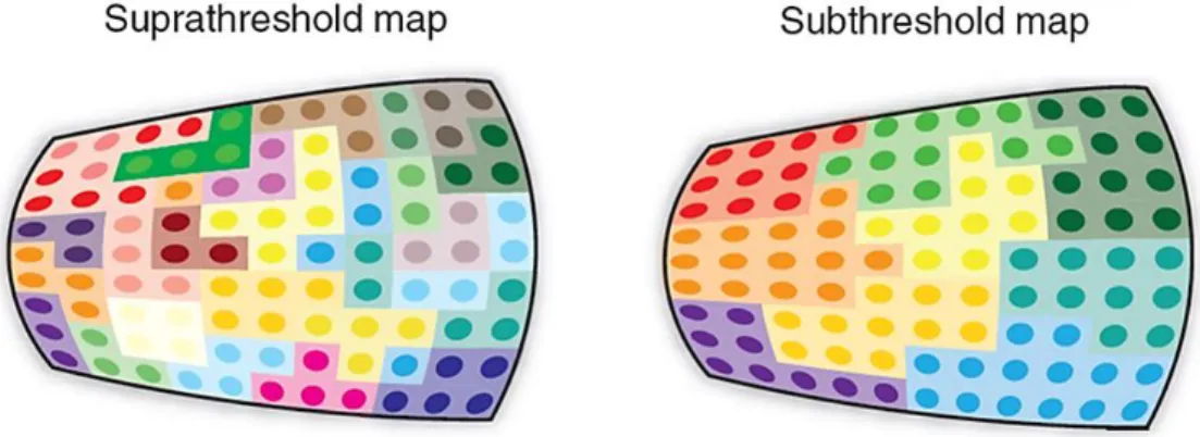
Figure 1-12. Schematic tonotopy of superficial layers in the mouse AI.
Tonotopic organization derived from two photon calcium recordings in anesthetized mice. Differences in suprathreshold and subthreshold activity account for a model of interconnected subnetworks with a fractured tonotopic organization based on best frequency tuning characteristics. Adapted from Castro and Kandler (2010).
Other stimulus representations in auditory cortex
Cortical maps are efficient for reducing complexity and redundancy, and enhancing coding power by coordinated parallel processing of the incoming sensory information (Chklovskii and Koulakov, 2004). Different sensory features are thought to be transformed in overlaid maps of sensory processing subnetworks that work together in order to generate single sensory percepts. Apart from the tonotopic organization previously described, there is evidence that other sensory features are mapped through the auditory system of birds, such as source location in the owl (Knudsen, 1984) and object distance in the bat (O’Neill et al., 1989). In the mammalian brain there have been reports of response maps of latency (Mendelson et al., 1997), sound intensity (Heil et al., 1994), amplitude and frequency modulations in a large variety of species (e.g.Clarey et al., 1994; Eggermont, 1998; Godey et al., 2005; Issa et al., 2017; Mendelson et al., 1993; Zhang et al., 2003) and binaural interactions in almost all of the species that haven been studied (Schreiner and Winer, 2007), including mice (Panniello et al., 2018). How these cortical maps interact is a matter of debate and active research (King et al., 2018), even though some theories have been presented such as the observations that neurons tuned to low frequencies would prefer sweeps going from low to high frequencies and the contrary, that neurons tuned to high frequencies would respond more often to sweeps in the opposite direction (Godey et al., 2005; Zhang et al., 2003). Technical limitations in conjunction with changing cortical states, due to different attentional states of the animals, during the course of long mapping experiments (Fritz et al., 2003) or task-specific
24
modulations(Bartlett and Wang, 2005; Scheich et al., 2007) have been largely detrimental for the correct mapping of auditory features and their interpretation. It has been observed that even looking at the same neuron, it can show in a short period of time a high ambiguity in its response profile (Schreiner and Winer, 2007).
Laminar organization
Looking in more detail, besides the columnar organization of the neocortex, there is a hierarchically laminar organization parallel to the pial surface which is the result of radial waves of migration of post-mitotic neurons during development. During early stages of development, neuroepithelial cells lining in the ventricles transform into radial glial progenitors (RGP), the main neuronal progenitor cell type responsible for the production of other progenitors and eventually for the final neuronal output (Purves, 2004; Uzquiano et al., 2018). At early stages, radial glial cells self-amplify in order to increase the progenitor pool. Progressively they produce other type of progenitor cells, namely basal progenitors. Humans brains are characterized by abundant basal radial glial progenitors, which are highly proliferative and thought to be important for neocortical expansion and evolution. In rodents, basal progenitors are mainly constituted by intermediate progenitors, dividing symmetrically and producing post-mitotic neurons (Douglas and Martin, 2007; Uzquiano et al., 2018). This last mentioned cell type, residing in the ventricular zone (VZ) of the dorsal telencephalon, enters into numerous rounds of symmetric division, generating different types of newborn neurons which in turn, migrate radially and differentiate producing the final columnar organization of the neocortex (Kornack, 2000).
25
Radial migration is observed during early development when new born neurons, from radial glial progenitors at the ventricular zone, migrate to the cortical plate and proliferate forming the layers of the cortex in an ‘inside-out’ manner. Adapted from Moffat and colleagues(2015).
The different layers are grouped into three parts: (1) supragranular layers containing layers from I to III, (2) internal granular layer comprising only the layer IV, (3) andinfragranular layers covering the layers V and VI. Although there is intricate connectivity between layers in a feedforward and feedback manner, the amount and type of cellular populations allows us to determine in part the functional role of each of these layers. In general terms in primary auditory areas, the information arrives mainly into layer IV, from which is broadcast to other cortical layers. Recordings of sound onset latencies in the different layers can account for this as smaller latencies are usually observed in layer IV with gradual increases towards the upper layers (Mendelson et al., 1997) (Figure 1-14). Layers II and III serve with intra-cortical and cortico-cortical projections whereas layers V and VI correspond to the main output layers to subcortical and other cortical structures. Although the functional impact and fine architectural features of all cortical layers has not yet been completely defined, there are some common rules that have been found in most mammals (Hackett et al., 2011).
Figure 1-14. Sound onset latency and recording depth for multi-units in AI.
The minimum sound onset latency for multi-units (MU) recorded across all layers of AI in the AC of cats plotted against cortical depth. The averaged approximate location of the cortical laminae is indicated with Roman numerals. Dashed line corresponds to averages of locally minimum onset latencies whereas the dotted line corresponds to the average onset latency