HAL Id: hal-00492039
https://hal-paris1.archives-ouvertes.fr/hal-00492039
Preprint submitted on 14 Jun 2010HAL is a multi-disciplinary open access archive for the deposit and dissemination of sci-entific research documents, whether they are
pub-L’archive ouverte pluridisciplinaire HAL, est destinée au dépôt et à la diffusion de documents scientifiques de niveau recherche, publiés ou non,
Inference on Time-Invariant Variables using Panel Data:
A Pre-Test Estimator with an Application to the
Returns to Schooling
Jean-Bernard Chatelain, Kirsten Ralf
To cite this version:
Jean-Bernard Chatelain, Kirsten Ralf. Inference on Time-Invariant Variables using Panel Data: A Pre-Test Estimator with an Application to the Returns to Schooling. 2010. �hal-00492039�
Inference on Time-Invariant Variables
using Panel Data: A Pre-Test Estimator
with an Application to the Returns to
Schooling
Jean-Bernard Chatelain
∗and Kirsten Ralf
†January 15, 2010
Abstract
This paper proposes a new pre-test estimator of panel data models includ-ing time invariant variables based upon the Mundlak-Krishnakumar estimator and an “unrestricted” Hausman-Taylor estimator. The paper evaluates the bi-ases of currently used restricted estimators, omitting the average-over-time of at least one endogenous time-varying explanatory variable. Repeated Between,
∗
CES, Centre d’Economie de la Sorbonne, Universit´e Paris I Pantheon Sorbonne, Paris School of Economics and CEPREMAP. 106-112 Boulevard de l’Hˆopital 75647 Paris Cedex 13. Email: [email protected]
†
Ordinary Least Squares, Two stage restricted Between and Oaxaca-Geisler esti-mator, Fixed Effect Vector Decomposition, Generalized least squares may lead to wrong conclusions regarding the statistical significance of the estimated pa-rameter values of time-invariant variables.
JEL classification numbers: C01, C22, C23.
Keywords: Time-Invariant Variables, Panel data, Time-Series Cross-Sections, Pre-Test Estimator, Mundlak Estimator, Fixed Effects Vector Decomposition.
1. Introduction
We observe in sample time-invariant variables such as variables of origin, rare events or rarely changing variables which have been measured only once within the period of interest. Let us give a few examples of time invariant variables: colonial, legal or political system, international conflicts, institutional and governance indicators, initial gross domestic product per head when testing the convergence of incomes in growth regressions; geographical position for cross country data in gravity models of foreign trade and foreign direct investments; years of schooling, gender and race when testing wage income using survey data. These variables are often highly relevant in a theoretical model predicting correlations with a cross-sections and time-varying variable of interest. Because publishing results that do not reject the null hypothesis of no effect of these time invariant variable on the time varying variable of interest is generally not accepted by journal editors, applied researchers are likely to select
estimators that reject the null hypothesis among the pool of available estimators. We are then interested in drawing inference with respect to the statistical signif-icance of these time-invariant variables (observed for N individuals) for explaining the variance of a time and individual varying variable (observed for N individuals during T periods). Since a time-invariant variable has no variance in the time direc-tion, it can only explain the variance of a time and individual varying variable in its individual direction. The reason why it matters for inference is that “the effect of a random component can only be averaged out if the sample increases in the direction of that random (time or individual) component” (Kelejian and Stephan 1983, see also Hsiao 2003, pp. 51-53.). For example, the pooled ordinary least square (OLS) esti-mator with time-invariant explanatory variables leads to inference on time-invariant variables using the time dimension N T . But “we have to deal with the unfortunate fact that there is not quite so much information in N individuals observed T times as there is with N T individuals.” (Johnston and Di Nardo (1997), pp. 395.).
This leads to the suggestion of a number of possible estimators for the parameter values with different characteristics. The available estimators of time invariant vari-ables using panel data or time series cross sections are found in Hausman and Taylor (1981), Hsiao (2003), Baltagi, Bresson and Pirotte (2003), Oaxaca and Geisler (2003), Krishnakumar (2006) extension of Mundlak (1978) and Pl¨umper and Troeger (2007) Fixed Effect Vector Decomposition Estimator (FEVD). For example, the FEVD es-timator has been widely used over the recent years (for example, Blaydes (2006)
and Goodrich (2006)). By contrast, the Mundlak-Krishnakumar (2006) estimator remained unnoticed by practitionners.
This paper suggests that inference on time-invariant variables without a pre-test Mundlak-Krishnakumar estimator may lead to conclude wrongly that time-invariant variables are statistically significant. This paper includes four contributions:
(1) It proposes a pre-test estimator based upon the Mundlak-Krishnakumar es-timator and a modified Hausman-Taylor eses-timator, extending the pre-test eses-timator proposed Baltagi, Bresson and Pirotte (2003).
(2) The Mundlak-Krishnakumar model is not currently used for doing inference on time invariant variables. It means that some currently published papers where the data generating process could be approximated by the Mundlak-Krishnakumar theoret-ical model report, for example, restricted estimators omitting the average over time of endogenous time-varying variables. The paper computes the determinants of the bias of the estimated parameters and of the estimated standard errors of using other esti-mators instead of the pre-test estimator. It presents an illustration of these omitted variable biases on a returns to schooling classic database (Baltagi and Khanti-Akom (1990), Cornwell and Rupert (1988), Baltagi (2008 and 2009), Cameron and Trivedi (2009), chapter 8).
(3 and 4) The paper explains why the Oaxaca-Geisler (2003) and FEVD estimators may provide misleading estimated standard errors of the parameters of time-invariant variables. Mitze (2009) and Breusch, Ward, Nguyen and Kompas (2010) found that
FEVD estimated standard errors of the estimated parameters of time invariant vari-ables were (too) small. The explanation that we propose is that the FEVD estimator uses the within root mean square error for the estimator of these standard errors. In so doing, it contradicts the Frisch-Waugh-Lovell theorem, where the same orthogonal projection matrix has to be used in the parameter estimate and in the estimator of its variance (following a similar argument, Greene (2010) refers to Aitken’s theorem). The overall picture is that when one uses this pre-test estimator, results may differ a lot from currently published inference which neglects a pre-test stage. There are two reasons for that. First, an omitted variable bias of the average over time of endogenous time-varying variables may occur. Secondly, the estimator of the standard error of the parameters of time invariant variables may be biased because of an excessive weight on within mean square error and on within degrees of freedom (depending on the time dimension T ). As the extent of these potential biases are not known when the data sets are not available for replication, this casts serious doubts on the emphasis put on inference on time invariant variable in panel data formerly published in academic journals.
This paper proceeds as follows. Section 2 defines our pre-test estimator based upon the Mundlak-Krishnakumar and the Hausman and Taylor estimator. Section 3 compares the outcome of different estimators using a typical time series cross section data set of gasoline demand. Section 4 analyses the differences of our pre-test estimator with the currently available estimators, in particular, the Oaxaca-Geisler, the two
stage, the FEVD and the usual random effects estimators. Section 5 concludes.
2. A Pre-Test Estimator including Time-invariant Variables
and Correlated Individual Effects
2.1. Mundlak-Krishnakumar Estimator
The model of time-series cross-sections regression estimates the following equation yit= Xitβ + Ziγ + αi+ εit (2.1)
where yit denotes the endogenous variable, Xit is a N T × k matrix of cross-sections
time-series data, Zi is a N T× g matrix of time invariant variables, β and γ are k and
g vectors of coefficients associated with time-varying and time-invariant observable variables respectively. Subscripts indicate variation over individuals (i = 1, ..., N ) and time (t = 1, ..., T ). Observations are ordered first by individual and then by time, so that αi and each column of Zi are N T vectors having blocks of T identical
entries within each individual i = 1, ..., N . The disturbance εit is assumed to be
uncorrelated with the columns of (Xit, Zi,αi) and has zero mean and constant variance
σ2ε conditional on Xitand Zi. The individual effect αiis assumed to be a time-invariant
random variable, distributed independently across individuals with variance σ2 α. The
primary focus of the literature is the potential correlation of αi with the columns of
Mundlak [1978] and Krishnakumar [2006] introduce an auxiliary regression which takes explicitly into account a linear relation between the explanatory variables and the individual random effects:
αi = Xi.π + Ziφ + αMi (2.2)
where it is assumed that the disturbance αM
i ∼ (0, σ2αM) and where Xi. is the average
over time for each individual of time varying variables, such that E³αM i | Xi.
´
= 0, π and φ are k and g vectors of coefficients associated with the average over time of time-varying variables and time-invariant observable variables, respectively. Clearly π = 0 and φ = 0 if and only if the time varying and time invariant variables are uncorrelated with the random individual effects. Combining the auxiliary regression with the initial regression yields:
yit= Xitβ + Zi(γ + φ) + Xi.π + αiM + εit (2.3)
When E (αi | Zi) = φ6= 0, one may only estimate the sum γ +φ and may not
iden-tify γ and φ separately, without additional prior information. The prior information the Hausman and Taylor (1981) procedure uses is the ability to distinguish columns of Xitand Zi which are asymptotically uncorrelated with αi from those which are not.
plim N →∞ 1 NX 0 1itαi = π1 = 0, plim N →∞ 1 NX 0 2itαi = π2 6= 0 plim N →∞ 1 NZ 0 1iαi = φ1 = 0, plim N →∞ 1 NZ 0 2iαi = φ2 6= 0
where Xit = [X1it, X2it] and Zi = [Z1i, Z2i] are split into two sets of variables such
that X1 is N T × k1, X2 is N T × k2, Z1 is N T × g1, Z2 is N T × g2 with k1+ k2 = k
and g1+ g2 = g. X1 and Z1 are assumed exogenous and not correlated with αi and
εit, while X2 and Z2 are endogenous due to their correlation with αi but not with
εit. The pre-test estimator proposed in the next section differs from the Hausman and
Taylor [1981] estimator in that no prior information is assumed about how to split π, but that the information is obtained using t-tests on each estimated parameter π ofb
equations (2.2) or equation (2.3).
It will prove helpful to recall the menu of conventional estimators for (β, γ) in equation (2.3). Letting iT denote a T vector of ones, two orthogonal projection
operators can be defined as:
B= IN ⊗
1 TiTi
0
T, W = IN T − B
which are idempotent matrices of rank N and N T−N respectively. With data grouped by individuals, B transforms a vector of observations into a vector of group means, such that By = y . Similarly, W produces a vector of deviation from group means:
i.e., Wyit = yit− yi.. For any time-invariant vector of observations, Wzi = O. The
orthogonality of the two projection operators is such BW = WB = ON T. The space
of observations (RN T) has an orthogonal decomposition in two spaces: the subspace of observations transformed by the between operator (dimension N ) and the subspace of observations transformed by the within operator (dimension N T−N). In other words, the covariance of the between transformed variable (time average for each individual i, with t a time index and T observations) xi. = T1 Pt=Tt=1 xit with respect to a within
transformation of another variable (yit− yi.) is always equal to zero:
cov (yit− yi., xi.) = 0 and cov (yit− yi., yi.) = 0 (2.4)
Hence, the total sum of squares SST of yit is the sum of total sum of squares
SSTW for the within transformed variable and T times the total sum of square SSTB
for the between transformed variable over N observations:
SST (yit) = SST (yit− yi.) + SST (yi.) = SSTW + T · SSTB. (2.5)
Transform model (3) by the Within projection operator, we obtain:
yit− yi. = WXitβ + WZi(γ + φ) + WXi.π + WαMi + Wεit (2.6)
Least square estimates of β in the within transformed equation are Gauss-Markov for the transformed equation and define the within-groups estimator:
b
βW = (X0itFXit)−1X0itFyit with F = W. (2.8)
Since the columns of WXit are uncorrelated with Wεit, βbW is unbiased and
con-sistent for β regardless of possible correlation between αi and the columns of Xit
or Zi. The OLS analysis of variance in the within subspace of observations (SSM
is the sum of squares of the model, SSE is the sum of squares of the error) is: SSTW = SSMW + SSEW. The sum of squared residuals (denoted form this equation
can be used to obtain an unbiased and consistent estimate of σ2 ε:
M SEW =σc2ε =
SSEW
N T − N − k (2.9) To make use of between-group variation, transform model (3) by the Between projection operator obtaining
yi.= Xi.(β + π) + Zi(γ + φ) + αMi + εi.
When E (αi | Xit, Zi) = 0 = π = φ, least squares estimates of β and γ in the
between transformed regression define the between groups estimators estimators (de-noted βbB and γbB) which are unbiased and consistent for β and γ, using N
observa-tions. When E (αi | Xit) 6= 0 or when π 6= 0 , βbB is biased and inconsistent. When
E (αi | Zi) 6= 0 or when φ 6= 0, γbB is biased and inconsistent. The OLS analysis
of variance in the between subspace of observations is: SSTB = SSMB + SSEB.
The sum of squared residuals SSEB provides a biased and inconsistent estimator for
var (αi+ εi.) = σα2i + (1/T ) σ
2
ε when E (αi | Xit, Zi) 6= 0 and unbiased and consistent
when E (αi | Xit, Zi) = 0. Whenever we have consistent estimators for both β and γ,
a consistent estimator for σ2
α can be obtained with:
M SEB =σc2α+ c σ2 ε T = SSEB N − k − g − 1. (2.10) Estimators that correspond to weighted average of the within and the between estimators are obtained as follows. Summing the within equation and the between equation multiplied by a parameter θ and repeated T times, which amounts to trans-form equation (3) applying the linear operator W+θB, we obtain:
yit− yi.+ θyi. = (W+θB) Xitβ + θZi.(γ + φ) + θXi.π + θαMi + (W+θB) εit (2.11)
When π 6= 0, that is when E (αi | Xit) 6= 0, and when E (αi | Zi) = 0 = φ,
Mundlak [1978] and Krishnakumar [2006] prove that the best linear unbiased estimator is obtained for a value of θ corresponding to the generalized least square model (GLS)
or random effect estimator, which leads to the following estimates: b βGLS = βbW, πbGLS =βbB−βbW and γbGLS =γbB, (2.12) var (πbGLS) = var ³ b βB ´ + var³βbW ´
and var (bγGLS) = var (γbB) (2.13)
A demonstration for the equalities on estimated variance-covariance matrix of esti-mated parameters is also found in Baltagi (2009, p.152-154). More precisely, Mundlak (1978) shows that (i) if αi is correlated with every column of Xi. (π6= 0, with k1 = 0
and k2 = k), the Gauss-Markov estimator for β is the within groups estimator βbW,
and (ii) if αi is uncorrelated with every column of Xi. (π = 0 in the true model, with
k1 = k and k2 = 0), the Gauss-Markov estimator for β is the “usual” GLS estimator
b
βGLS, (iii) Using the “usual” GLS estimate assuming the restriction π = 0 when the
true model is such that π 6= 0 is denoted “‘restricted GLS” (RGLS) and leads to biased estimate βbRGLS 6= βbGLS = βbW, because of the k omitted variables Xi. bias.
The estimator πbGLS is equal to the difference between the between estimator and the
within estimatorβb1,B−βb1,W.
For the time-invariant variables, the estimator γbGLS is exactly the between
esti-matorγbB. The standard error estimator, σbbγGLS, of the estimated parameter using the
Mundlak GLS model is exactly the same as the one of the between regression (see appendix 1). This estimator — even though the data includes N T observations — takes into account that for time-invariant explanatory variables only N observations should
be used. It has N − k − g − 1 degrees of freedom: b σbγGLS =σbbγB = s SSEB N − k − g − 1 1 q CSS(zj) q 1− R2 A(zj) , for j = 1, ..., g (2.14) where CSS is the sum of squares corrected for the mean and 1− R2
A(zj) is the
“tolerance” (or the inverse of the variance inflation factor) and where R2
A(zj) is the
coefficient of determination of the following auxiliary regression where the explanatory variable zi is explained by all other explanatory variables of regression (3) in the
between dimension (Stewart 1987):
zj = Xi.π0+ Zi,−jγ0+ η
0
j
where η0j are disturbances, where π0and γ0 are coefficients, and where Zi,−j is the
matrix of time-invariant variables excluding the column of observations related to the variable zj. R2A(zi) measures the effect of other explanatory variables on the
estimated standard error of the estimated parameter of a given variable zi. When
R2
A(zi) is close to unity, there is a potential problem of near-multicollinearity. The root
mean squared error of the between regression (including the degrees of freedom in the denominator) isq SSEB
N −k−g−1. The convergence of the estimator is obtained by increasing
N to infinity, for T fixed. An increase of T does not lead the between estimator to converge. Inference on time-invariant explanatory variables do not depend on the number of observations in the time dimension T .
2.2. A Pre-test Estimator
The pre-test estimator consists of a first step using the Mundlak-Krishnakumar esti-mator (equation (2.3) using GLS method) and then perform specification tests of null hypothesis H0 : E (αi | Xmit) = πm = 0 against the alternative H0 : E (αi | Xmit) =
πm 6= 0 for each of the time-varying explanatory variables 0 ≤ m ≤ k. If H0 is rejected
for exactly k2 variables, these variables are included in the subset X2it assumed to be
endogenous due to their correlation with αi but not with εit, while the remaining
k1variables are included in the subset X1it. Hence, no prior information on how to
split Xit is required for this pre-test estimator. In practice, researchers priors on how
to split Xit and Zi based on theory may be misleading because of unobservable and
omitted time-invariant variables, measurement errors, and so on.
The second step consists of using an unrestricted Hausman Taylor (1981) estimator using X1it as instruments for Z2 endogenous time invariant variables, but keeping the
time invariant variables X2i.. which are not used as instruments, in order to correct for
their endogeneity (this is not usually done with the Hausman and Taylor estimator). More precisely, if the specification tests rejects H0 for k2 ≥ 1 variables, it may still
be possible to obtain consistent estimates of both β and γ in a second stage. Let
b di = yi.− Xi.βbW = ³ B− Xi.(X0itWXit)−1X0itW ´ yit
Ex-panding this expression using equation 2.3 including only X2i.leads to:
b
di = Z1i.γ1+ Z2i.(γ2+ φ2) + X2i.π2+ αMi +
³
B− Xi.(X0itWXit)−1X0itW
´
εit. (2.15)
Treating the last two terms as an unobservable mean zero disturbance, consider estimating γ from the above equation using N observations. If αiis correlated with the
columns of Z2i, E (αi | Z2i) = φ2 6= 0, according to prior information, both OLS and
GLS will be inconsistent estimates for γ. Consistent estimation is possible, however, if the columns of X1it, uncorrelated with αi according to the non rejection of the null
hypothesis of preliminary tests, provide sufficient instruments for the columns of Zi.
in equation (4.1). A necessary condition for identification of γ2 and φ2 is that k1 ≥ g2:
there are at least as many exogenous time-varying variables as there are endogenous time-invariant variables (proposition 3.2 in Hausman and Taylor (1981)). When the condition k1 ≥ g2 is fulfilled, one may proceed to a second step for estimating γ
knowing that the first step provided efficient estimates of β.
The two stage least squares (2SLS) estimator for γ in equation (4.1) is:
b
γII = ([Z0i, X2i.] PA[Z0i, X2i.])−1[Z0i, X2i.]0PAdbi (2.16)
where A = [X1it, Z1i] and PA is the orthogonal projection operator onto its column
b
γII−γ = ([Z0i, X2i.] PA[Z0i, X2i.])−1[Z0i, X2i.]0PA
³
αMi +³B− Xi.(X0itWXit)−1X0itW
´
εit
´
and under the usual assumptions governing Xit and Zi, the 2SLS estimator is
consis-tent for γ, since for fixed T , plimN →∞N1A0αi = 0 and plimN →∞N1X
0
itεi = 0. Having
consistent estimates of β and, under the condition k1 ≥ g2, γ, we can construct
con-sistent estimators for the variance components. A concon-sistent estimate of σ2
ε can be
de-rived from the within-group residuals in the first stepσc2
ε = M SEW. Whenever we have
consistent estimators for both β and γ, a consistent estimator for σ2
α can be obtained. Let s2 = (1/N ) ³Y i.− Xi.βbW − ZiγbII − X2i.πb2,II ´0³ Yi.− Xi.βbW − ZibγII− X2i.πb2,II ´ : then plim N →∞ s2 =plim N →∞ 1 N (αi+ εi) 0(α i+ εi) = σα2 + 1 Tσ 2 ε so that s2 a= s2− (1/T ) s2ε is consistent for s2a.
In the particular case when one assumes that αiis uncorrelated with the columns of
Zi: E (αi | Zi) = 0 = φ, and when all time varying variables reject the null hypothesis
H0 (k1 = 0) using N observations to estimate the above equation in a second stage II,
both OLS and GLS will be consistent estimates of γ identical to the between estimates (γbII,OLS =γbB, σbbγII,OLS =σbbγB ) and with πbII,OLS =βbB−βbW.
random effects estimator if the standard Hausman test based on the “within-groups” versus the random effects estimators is not rejected. It reverts to the HT estimator if the choice of strictly exogenous regressors is not rejected by a second Hausman test based on the difference between the “within-groups” and HT estimators. Otherwise, this pre-test estimator reverts to the “within-groups” estimator.
The pre-test estimator differs from BBP (2003) in that (1) it assumes Mundlak auxiliary regression, (2) it tests the endogeneity of each time-varying variables instead of relying on prior information for splitting Xit = [X1, X2], (3) it includes X2i.π2which
may change widely the estimates of γ in the second stage, (4) when 0≤ k1 < g2 (not
enough exogenous X1itto instrument endogenous Z2i ) or respectively when g2 = 0
and k1 = k (no endogenous Z2i, and all time varying variables are endogenous X1it)
it reports a biased (respectively unbiased) estimators for γ, instead of no estimates at all.
Because classical statistical hypothesis testing implies non-zero probabilities of type I error (p-value) and type II error (one minus the power of the test), a pre-test estimator cannot perform as well as an estimator where the researcher exactly knows the “true” model based on “true prior information” before testing. This only occurs when the number of observations tends to infinity, so that the probabilities of both types of errors tends to zero.
Mundlak (1978) considers the following estimators for his theoretical model: pooled OLS (θ = 1), between, within (θ = 0), Generalized least square (GLS) or random
effects estimator (for an estimated value of θ), restricted generalized least square with the restriction π = 0 (that is applying the usual random effect model whereas the true model is such that: π 6= 0), restricted pooled OLS with the restriction π = 0. The reasons for considering restricted estimators are twofold. Firstly, these restrictions are likely to decrease the variance of the estimators although these restricted estimators are generally biased. There is therefore a trade off between bias and variance and the choice of an estimator depends on the weights to be assigned to the two components. Secondly, the Krishnakumar-Mundlak is not currently used for doing inference on time invariant variables. It means that some currently published papers where the data generating process could be approximated by the Mundlak theoretical model report Mundlak’s restricted estimators. It is interesting to evaluate the bias of the estimated parameters and of the estimated standard errors of the time invariant variables for the restricted models. We therefore do a similar investigation as Mundlak (1978) did on retricted estimators for time varying variables, and we focus on the estimators related to time-invariant variables when our pre-test is estimator is consistent.
3. A Return to Schooling Illustration of the Unrestricted Model
3.1. Pre-test Estimator
The pre-test estimator leads to dramatic changes with respect to alternative estimators of time invariant variables in panel data. This is demonstrated empirically for a return to schooling example based on a panel of 595 individuals observed over the
period 1976-1982 drawn from the Panel Study of Income Dynamics (PSID) (Baltagi and Khanti-Akom (1990), Cornwell and Rupert (1988)). First, the tests based on Mundlak-Krishnakumar specification lead to alternative choices of the instruments than the ones chosen by Baltagi and Khanti-Akom (1990) and Cornwell and Rupert (1988). Second, when the average over time of endogenous time varying variables are not omitted in the Hausman-Taylor estimates, the estimates of the return to schooling are much lower than the ones found by Baltagi Khanti-Akom [1990] and Cornwell and Rupert [1988].
In tables 1 and 2, the dependent variable log(wage) is explained by nine time-varying variables (Xit’s) and three time-invariant variables (Zi’s). Baltagi and
Khanti-Akom (1990) and Cornwell and Rupert (1988) assumed that four of the Xit variables
and two of the Zi variables are uncorrelated with the individual effects. These are
denoted by X1 and Z1, respectively. They are listed at the bottom of table 2. The
remaining Xit and Zi are correlated with the individual effects. They are denoted by
X2 and Z2, respectively.
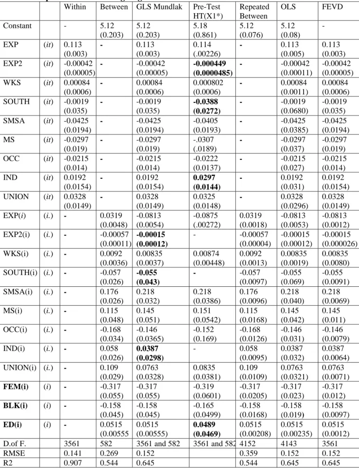
Table 1 includes estimates of the unrestricted model using six estimators: within, between, Mundlak-Krishnakumar, pre-test unrestricted Hausman-Taylor, repeated be-tween (RB), ordinary least square (OLS) and FEVD. Table 2 includes six estimates of the restricted model: step II restricted between, step II repeated restricted between, GLS, OLS, FEVD and HT(X∗∗
X∗∗
1 is the one chosen by Baltagi and Khanti-Akom (1990). 1
For the unrestricted model, we observe the following. The estimates of the all parameters are identical for all estimators, except for the average over time of a time-varying variable in the Between or Repeated Between estimators which exclude the time- and individual-varying variable. For the time- and individual-varying variable, Mundlak-Krishnakumar, LSDV and FEVD estimators exhibit the same estimated standard deviation and value of the t-statistics, which differs from OLS. But, for the time-invariant variable, the estimated standard deviation and the values of the t-statistic vary dramatically. For the Between and the Mundlak-Krishnakumar estima-tors, the estimated standard deviations of time invariant variables are equal, whereas the estimated standard deviations for the repeated between estimate are 2.67 times smaller, the ones for the OLS estimate are 2.33 times smaller, and the ones for the FEVD estimate are 4.63 smaller. It seems, and this is confirmed later on by our the-oretical analysis, that the standard deviation of the OLS and FEVD is systematically smaller and the value of the t-statistic systematically larger than for the Mundlak es-timator. If this is the case, inference with the OLS and FEVD estimator will less often reject the null-hypothesis that γ is equal to zero, and more often conclude that the time-invariant variable has an effect on the endogenous variable statistically different from zero.
In table 1, the within estimator, which is consistent, serves as a benchmark for the
1Five of these thirteen estimates are also reported in Baltagi [2009], p.27-29: Within, Between,
Hausman (1978) test. The experience variable (EXP) is a time trend which differs only in levels for each individuals, i.e. EXPit = EXPi.+ t where EXPi. is the average
number of years of experience in the sample of years 1976-1982 for each individual i and t is a time trend (= −3 for 1976,...,= +3 for 1982). This individual time trend accounts for 65% of the within variance of the dependent variable log(wage), along with a correlation coefficient of 0.8. Once this variable is included in the model, the partial R2 contribution of the eight other within transformed variables is very small (the R2 increases by only 0.74%). The estimated coefficients of blue collar occupation (OCC), of marital status (MS), of living in the south of the U.S.A. (SOUTH), of weeks worked (WKS), of industry (IND), of the standard metropolitan statistical area (SMSA), of belonging to an union (UNION) and of EXP2 are statistically significant.
The between estimator includes estimates of the three time invariant variables: female workers (FEM), black worker (BLK), and years of schooling (ED). Degrees of freedom are 582. All the estimated coefficients are statistically significant. The 95% confidence interval for the return to school is [0.045, 0.057]. The standard error estimator, σbbγGLS, of the estimated parameter using the Mundlak-Krishnakumar GLS model is exactly the same as the one of the between regression (table 1, column 2):
b σbγGLS =σbbγB = q SSE B N −k−g−1 q CSS(zi) q 1− R2 A(zj) = q42.07257 595−13 √ 4623.77479 1 √ 0.50673 = 0.00555 where 1− R2A = 0.5067 is the tolerance and CSS is the sum of squares corrected for
The Mundlak-Krishnakumar estimator is able to deal with a non linear model (this one includes EXP2) as long as the model remains linear with respect to the
parameters. It provides t-tests for parameters of the average over time of the nine time-varying variables, indexed by m (H0 :πbGLS,m =βbB−βbW). At the 5% threshold,
these tests accept the null hypothesis for the parameters of the variables X∗
1 = (EXP2,
SOUTH, IND) which is the choice of exogenous variable of the pre-test estimator. It is remarkable that EXP is strongly endogenous in the sample whereas EXP2 is
exogenous in the sample. Cornwell and Rupert [1988] assumed that X1 = (SOUTH,
WKS, SMSA, MS) are exogenous. Baltagi and Khanti-Akom (1990) assumed that X∗∗
1 = (SOUTH, IND, OCC, SMSA) are exogenous. However, the t-statistic in the
Mundlak parameter is equal to t = 4.01 for OCC and to t = 6.77 for SMSA. The choice of exogenous time-invariant variables is based on prior assumption: Z1 = (FEM,
BLK). Years of education Z2 = (ED) is assumed to be correlated with the individual
effect.
In column 4, the pre-test unrestricted Hausman Taylor estimator using X∗1 as
in-struments of Z2 = (ED) and including the average over time of endogenous time
varying variables X∗
2 = (EXP, WKS, SOUTH, SMSA, MS, OCC, UNION) leads to
larger estimates for SOUTHit and for INDit than with the consistent within
estima-tor. The return to schooling estimates (0.049) is nearly the same than the Between estimator (0.051). However, it is no longer statistically significant, with a 95% con-fidence interval equal to [−0.05, 0.15], to be compared with the Between estimator
[0.045, 0.057].
This lack of precision is partly due to the fact that X∗
1 consists of three weak
instruments explaining altogether only 12% of the variance of years of education. The pre-test estimator leads to choose highly exogenous instruments X1. If the variables
Z2 are strongly correlated with unobservable heterogeneity αi, then the exogenous
instruments X1 will be weakly correlated with Z2. Because the pre-test estimator
leads to choose weak instruments, the Mundlak estimator is likely to be as reliable as the Hausman-Taylor estimator for this data set.
3.2. Repeated Between Estimator
We present this estimator because repeating T times the time invariant observations turns out to be the major component of the increase of the t-statistic of time-invariant variables using panel data for several other estimators. However, Kelejian and Stephan (1983) argue “the effect of a random component can only be averaged out if the sample increases in the direction of that random (time or individual) component”. By con-trast, Oaxaca and Gleiser (2003) assume that the consistency of the estimator of a parameter of a time-invariant explanatory variable “depends on the time series obser-vations approaching infinity”. The estimated parameters of time-invariant variables are the same with the repeated between and the between estimator (γB = γRB). The
to (the subscript for this estimator is RP B): b σbRBγ = q T ·SSEB N T −k−g−1 q T · CSS(zj) 1 q 1− R2 A(zj) = s N− k − g − 1 N T − k − g − 1σb B bγ = b σbγB 2.671.
Inference uses N T−k−g −1 degrees of freedom instead of N −k −g −1 in the between estimator. The coefficient of determination of the auxiliary regression R2
A(zj) does not
change in the between or repeated between samples. The estimated standard error of the estimated parameter of the time invariant variables is divided byq4165−13
595−13 = 2.67
in table 1. As the parameter estimate is the same as γB, the repeated between tRB -statistic amounts to multiply the between tB statistics by the following factor:
tRB = γc B b σRB c γB = s N T − k − g − 1 N − k − g − 1 c γB b σB b γ = s N T − k − g − 1 N − k − g − 1 t B
When N is large, the t-statistic of the repeated between model is multiplied by around√T (say by 2 when T = 4 and by 5 when T = 25) with respect to the between model.
3.3. Pooled OLS Unrestricted Estimator
The Pooled OLS (θ = 1) estimator ignores the random effects. It leads to the same parameter estimates as the Mundlak estimator, but not the same standard error es-timates. The reason why we analyse the Pooled OLS estimator for time-invariant explanatory variables is that it is still used by some applied researchers. When
test-ing does not reject the existence of random effects and when the Hausman test leads to reject the random effect models with respect to the “correlated random effects” model, some applied researchers present Pooled OLS estimates with time invariant explanatory variables, on the ground that the required within estimates wipes out time-invariant variables. For example, Oaxaca and Geisler [2003] evaluate the consis-tency of the OLS estimator of a parameter of a time-invariant explanatory variable.
The OLS estimator uses the irrelevant N T − k − g − 1 degrees of freedom for time-invariant variables. The estimated standard error is larger than for the repeated between estimator, because the RM SE of the OLS estimator is larger since it includes the sum of squares of the error of the within model: SSEOLS = T · SSEB+ SSEW
(the last equality presents table 1 values):
b σbOLSγ = q T ·SSEB+SSEW N T −k−g−1 q T · CSS(zi) 1 q 1− R2 A(zj) = s 1 + SSEW T · SSEB s N − k − g − 1 N T − k − g − 1σb B b γ. = s 1 + 84.11480 7· 42.07257 = 1.1338· b σB bγ 2.671 = b σB bγ 2.33. R2
A(zj) is the determination coefficient of the auxiliary regression. It does not
change with respect to the between, repeated between and OLS estimators. In table 1 example, as T = 7 is small, the OLS tOLS statistics (equal to 2.33 times the between
tB statistics) is close to the repeated between tRB statistics (equal to 2.67 times the
variance of the within transformed explained variable, taking into account SSEW is
irrelevant for doing inference on time-invariant variables.T
4. The Omitted Variable Bias of the Restricted Models
4.1. Restricted Random Effect Estimator
Both, the restricted random effects and the Mundlak-Krishnakumar estimator use the same weight θ for computing quasi demeaned variables (the second equality refers tob our example) using the Swamy and Arora method (1972):
yit− yi.+θyb i. with θ =b RM SEW √ T · RMSEB = √0.14071 7· 0.26887 = 0.1978.
The between regression includes the same variables (the average-over-time of all explanatory variables. Hence, the root mean squared error of the between estimator RM SEB is the same in both models. The restricted random effect model faces an
omitted variable bias when one rejects the null hypothesis βbB =βbW, for at least one
time-varying variable. In the wages example, the bias with the random effect model is (γGLS denotes the Mundlak GLS estimator whereas γRGLS denotes the Mundlak
restricted GLS estimator): b γRGLS =γbB+ j=k X j=1 ³ b βB−βbW ´ b βbθx i./bθzii = 0.06966 + 0.03044 = 0.10
with βxi./zi given by the auxiliary regression using OLS on quasi demeaned variables (table 2, column 1): b θxi. = βxi./ziθzb i+ βxi./xit ³ b θxi.+ xit− xi. ´ +θβb 0+ εit.
The omitted variable bias on the parameters of the time-invariant variables is large for ED (the return of education parameter nearly doubled: it is multiplied by 1.93βB)
and it is smaller for BLK (1.33βB)and FEM (1.06βB). The omitted variable bias on
the t-statistic is 1.87tB for ED, 1.03tB for BLK, 1.14tB for FEM. 4.2. Restricted Hausman-Taylor Estimator
In table 2, the column HT(X∗∗
1 ) presents Baltagi and Khanti-Akom (1990) estimates
using the standard Hausman Taylor procedure, with the set of instruments X∗∗ 1 and
omitting the average-over-time of the endogenous time-varying variables X∗∗ 2 . The
return to schooling is 0.137 with a confidence interval [0.116, 0.158].
The rise of the return to schooling with respect to the between estimate is only partly due to “instrumental variables” correcting the endogeneity of schooling with the individual effect. Around half of the rise is given by the omission of time-invariant variables which corrects the endogeneity of time varying regressors with the individual effect. The other component of the rise of the parameter is related to the strong instrument “blue collar occupation” which is strongly correlated with the number of years of education (its correlation coefficient around 0.45). This is likely to drive the
results emphasized by Boumahdi and Thomas [2006] for their measure of instruments relevance on this data set. They find that the gain in efficiency across the various sets of instruments seems to be in the education variable. However, “blue collar occupation” is endogenous, with a relatively large difference between its estimated parameters βbB − βbW with a relatively large t statistics (t = 4.57) in the Mundlak
equation. Unobservable ability affect primarily the number of years of education, which determine the outcome of a “blue collar” occupation.
Let us finally remark that Angrist and Pischke (2009, p.64-68) do not recommend to include the time varying variable OCCit (occupation) when investigating the causal
link between education and wages, because it is an outcome variable which occurs at a later stage than education.
4.3. Two-stage Restricted Between
A common practice consists of a two-stage restricted between (denoted II − RB) estimator of time-invariant variables, with the restriction β =b βbW for the
average-over-time of time-varying variables in a between regression. Let
b di = yi.− Xi.βbW = ³ B− Xi.(X0itWXit)−1X0itW ´ yit
be the N vector of group means estimated from the within-groups residuals. Expand-ing this expression leads to:
b di = Z1i.γ1+ Z2i.(γ2+ φ2) + αiM+ ³ B− Xi.(X0itWXit)−1X0itW ´ εit+ Xi. ³ b βB−βbW ´ (4.1) Treating the last two terms as an unobservable mean zero disturbance, consider estimating γ from the above equation using N observations, without taking into ac-count that the disturbances of the restricted between includes this omitted term: Xi.
³ b
βB−βbW
´
. There is then an omitted variable bias on the parameter of the time-invariant variable: b γII−RB =γbB+ j=kX j=1 ³ b βB−βbW ´ b βxj./zi
with βxi./zi estimated using the following auxiliary regressions in the between
dimen-sion:
xi. = βxi./zizi+ β0,xi./zi + εi,xi./zi.
In this two stage restricted between estimator, the omitted variable bias on the estimated standard error of the estimated parameter of the time-invariant variables leads to differences with respect to the between estimator:
b σbγ2 II−RB = s SSEII−RB N − g − 1 1 q CSS(zi) q 1− R2 A,RB(zj) 6= b σbγB = s SSEB N− k − g − 1 1 q CSS(zi) q 1− R2 A(zj)
First, the sum of squares of errors SSEII−RB is larger than the SSEB because the
model constrains the parameters of the time-varying variables to their within estimate which may not minimize the between sum of squares of errors. However, this increase of the estimated standard error may be offset for two reasons due to the fact the averages of k time-varying variables are on the left hand side of the equation. First, the degrees of freedom increase by k. This decreases the root mean squared error. Second, the variance inflation factor decreases because R2
A,RB(zj) < R2A(zj). R2A(zj)
is the coefficient of determination of an auxiliary regression where the time-invariant variable is correlated with the other g− 1 time-invariant explanatory variables on the right hand side of the equation. In the between estimator, R2
A(zj) is the coefficient of
determination of an auxiliary regression where the time-invariant variable is correlated with the other g−1 time-invariant explanatory variables and k averages of time-varying explanatory variables. As the number of explanatory variables increases by k, one has R2
A,RB(zj) < R2A(zj).
With respect to the estimated parameter of the non restricted between, the esti-mated parameter of the restricted between are multiplied by 0.89 for BLK, by 1.23 for ED and by 1.42 for FEM. With respect to the t-statistics of the non restricted between, the t-statistics of the restricted between are multiplied by 0.77 for BLK, by 1.47 for ED and by 1.86 for FEM.
Oaxaca and Geisler (2003) propose an alternative correction of the omitted variable bias of the two-stage restricted between approach than the Mundlak-Krishnakumar
estimator. They estimate the repeated restricted between with a two stage generalized least square estimator using a covariance matrix that takes into account that the disturbances of the restricted between includes this omitted term: Xi.
³ b
βB−βbW
´
. The first drawback of the Oaxaca and Geisler (2003) estimator is that the second step between should not be estimated using observations repeated T times. The second drawback is that it is simpler to include explicitly the variables Xi. in the
Mundlak-Krishnakumar estimator, than to compute a two stages GLS estimator with a specific covariance matrix.
4.4. Three-stage FEVD Unrestricted and Restricted Estimator
The FEVD estimator adds a third stage to the previous two stage estimator. It is assumed that time-invariant variables are not correlated with the random individual effects: E (αi | Zi) = φ = 0 and three sets of alternative assumptions can be dealt
with (E (αi | Xit) = π = 0, or E (αi | X2it) = π2 6= 0 or E (αi | Xit) = π 6= 0 (all
time-varying variables are endogenous). Pl¨umper and Troeger (2007) use a restricted FEVD estimator with a second stage and a third stage omitting variables X2i. or Xi.
which is consistent with the assumption E (αi | Xit) = π = 0. Note that if αi is
random instead of being fixed, the “usual” GLS estimator is consistent, which is not the case of the first stage “within-groups” estimator for the FEVD.
Let us denote εbi,B the between residuals of stage II restricted between:
b εi,B =αbiM+ ³ B− Xi.(X0itWXit)−1X0itW ´ b εit+Xi. ³ b βB−βbW ´ = yi.−Xi.βbW−Zi.γbII−RB
The third stage of the FEVD estimator is an OLS regression which includes the residual of the second stage repeated between regression denotedεbi,B with a parameter
δ estimated or constrained to one.
yit = Xitβ + Ziγ + Xi.π +εbi,B· δ + ηit,III.
Expanding this expression yields: yit− yi. = Wyit= (Xit− Xi.) β− Xi.
³
β− δβbW
´
+ Zi(γ− δγbII−RB) + ηit,III (4.2)
Wyit is orthogonal in the sample to all time-invariant variables, so that OLS estimates
are: γ =b δbγbB, π =b δb ³ b βB−βbW ´ , β =b δβb W, β =b βbW, δ = 1, andb ηbit,III = εbit −εbi..
The residuals of the third step regression are exactly the within-groups regression residuals. The only change of the three stage FEVD estimator with respect to the two stage estimator is related to the estimated standard error of the parameters γ of time invariant variables Zi. The FEVD estimator of the standard error of the
estimated parameter of a time-invariant variable amounts to substitute the mean squared error in the between dimension (M SEB = SSEB/ (N− k − g − 1)) by the
mean squared error in the within dimension (M SEW = SSEW/ (N T − N − k)). The
estimated parametersγbII−RB are related to the projection in the between subspace of observations, but their estimated standard errors are related to the projection in the within subspace of observations, which is orthogonal to the between subspace. This
contradicts the Frisch-Waugh-Lovell theorem: the same orthogonal projection matrix has to be used in the parameter estimate and in the estimator of its variance.
The Frisch-Waugh-Lovell decomposition of the Between and the Within dimen-sion holds with any of these assumptions: effects are fixed or random, or the time-varying variables are correlated or not with the random effect do not matter at all. As the residuals in the between dimension are excluded from the computation of the variance of the parameters, the potential correlations of the time-invariant variable with the individual random effect (which are in the between dimension) are excluded from the computation of the FEVD variance of the parameters. As well, adding a large number of time-invariant variables in the regression, in particular when they are near-multicollinear with the time-invariant variable of interest, changes the estimated parameter, but does not increase the FEVD estimated standard error of the estimated parameter of the time-invariant variable of interest. So the FEVD wipes out near-multicollinearity problems in the time-invariant dimension, which is also “practical” for reducing estimated standard errors.
This analysis explains why Kristensen and Wawro 2007 (footnote p.22) found that the FEVD estimated standard errors were relatively “too small” using Monte Carlo simulations with respect to other estimators. The FEVD estimator of the standard error is (the last equality refers to the unrestricted FEVD case, table 1 column 6):
b σbγF EV D = q SSEW N T −N−k q T · CSS(zi) 1 q 1− R2 A(zj) = s N − k − g − 1 N T − N − k s SSEW T · SSEB b σbγB
= s 595− 13 4165− 595 − 9 s 84.11480 7· 42.07257σb B b γ = 1 2.4736 · 1 1.8712 ·σb B b γ = b σbBγ 4.6286 The FEVD estimated standard error of a time-invariant variable is usually biased downwards for two reasons:
- It uses N T− N − k degrees of freedom (with N the number of individuals, k the number of time-varying explanatory variables, with T the number of periods) instead of N − k − g − 1 degrees of freedom.
- It multiplies the repeated between estimator of the standard error by a positive factor q SSEW
T ·SSEB which can be much smaller than one when T increases.
The combination of the potential omitted variable bias of the parameter estimate of the time invariant variable ED in the restricted between (step II) and of the bias of the estimated standard error implies a t-statistics equal to tRF EV D = 5.69 · tB
times the t-statistics of the Mundlak model for the restricted FEVD (table 2, column 6). For the unrestricted FEVD (table 1, column 6), only the bias of the estimated standard error matters, so that the tF EV D = 4.62· tB times the t-statistics of the
Mundlak model for ED. For the time invariant BLK, tRF EV D = 3.6· tB and for FEM,
tRF EV D = 8.6· tB. Note that when T corresponds to an aggregate annual time series
(T = 25,√T = 5), the increase of t-statistics is effect is likely to double with respect to the wages example (T = 7,√T = 2.6). Mitze [2009] also finds that the FEVD estimator tends to have a smaller root mean square error (rmse) than both Hausman-Taylor models with perfect and imperfect knowledge about the underlying correlation
between right hand side variables and residual term. Nonetheless, concluding that FEVD is “more efficient” is misleading, because the computation of the estimated standard errors of estimated parameters contradicts Frisch-Waugh-Lovell theorem.
5. Conclusion
Our theoretical and empirical investigation on inference on time-invariant variables shows that a pre-test estimator based upon the Mundlak-Krisnakumar and a modified Hausman-Taylor estimator should be used. Furthermore, the procedures are already programmed and available in all econometric softwares. The first stage consists of the usual random effects GLS estimator including all the variables Xi.. The second
stage uses instrumental variables X1i. keeping the X2i. as explanatory variables, using
instrumental variables estimator or the Hausman-Taylor estimator procedures. An example shows first that a time-invariant variable is not statistically significant for some estimators and highly statistically significant with other estimators.
The Mundlak-Krishnakumar regression reports within estimates and between esti-mates, with tests of the null hypothesisβbB−βbW = 0 for each time-varying explanatory
variable. In the case where at least one (but not all) xi. have estimated parameter
b
βB−βbW small and not significantly different from zero, the Mundlak estimator
sug-gests which of the xi. is exogenous. Then, these exogenous xi. are the ones to be used
as instrumental variables in a variant of the Hausman and Taylor [1981] instrumental variables estimator, including the average over time of endogenous time-varying
vari-ables. Using this pre-test estimator, one does not rely on subjective priors for deciding which time-varying variables are or are not endogenous in the Hausman and Taylor estimator.
One may try further Chamberlain (1984) estimators where the correlation of ex-planatory variables with the random individual effects is not only contemporaneous, but can also be related to leads and lags of explanatory variables.
It is not necessarily the failure of a model that the outcome of the tests is: ¯¯¯ bβB
¯ ¯ ¯>
b
βW = 0. Some variables have zero or small correlation coefficients in the within
subspace, and large correlation coefficients in the between dimension, just because it is the statistical information included in these rarely changing or time-invariant variables during the period of observations in available data sets. If we turn to the case of rarely changing variables instead of time-invariant variables, these variables are characterized by small within correlation coefficients with the explained variable and with all other explanatory variables. By contrast, they may have high between correlation coefficients with the explained variable and with all other explanatory variables. The variables are typically such that the null hypothesis βbB − βbW = 0
is rejected. The Mundlak estimator provides directly the t-test related to this null hypothesis. It is of particular interest for those variables, which are likely to be endogenous and significant variables in the Mundlak approach. If ever they do not have large between correlation coefficients, then the joint hypothesis βbB = βbW = 0
References
[1] Angrist J.D. and Pischke J.-S. [2009]. Mostly Harmless Econometrics. Princeton University Press, Princeton.
[2] Baltagi B. H. [2008]. Econometric Analysis of Panel Data. Fourth Edition, Wiley, Chichester.
[3] Baltagi B. H. [2009]. A Companion to Econometric Analysis of Panel Data. Wiley, Chichester.
[4] Baltagi B. H. and S. Khanti-Akom [1990]. On efficient estimation with panel data: an empirical comparison of instrumental variables estimators, Journal of Applied Econometrics, 5 pp. 401-406.
[5] Baltagi B. H., Bresson G. and Pirotte A. [2003]. Fixed Effects, Random Effects or Hausman-Taylor? A Pre-test Estimator. Economics Letters. 79 pp. 361-369. [6] Beck N. and Katz J. [2001]. Throwing out the baby with the bath water: a
comment on Green, Kim and Yoon. International Organization 55(2) pp. 487-495.
[7] Blaydes L. [2006]. Rewarding Impatience: A response to Goodrich. International Organization, 60, pp. 515-525.
[8] Boumahdi R. and Thomas A. [2006]. Instrument relevance and efficient estimation with panel data. Economics Letters, 93, pp. 305-310.
[9] Breusch T., Ward M.B., Nguyen H. and Kompas T. [2010]. On the fixed effects vector decomposition. Munich Personnal Repec Archive Paper 21452.
[10] Card D. [1999]. The Causal Effect of Education on Earnings. in Handbook of Labor Economics. Volume 3A. ed. by O. Ashenfelter and D. Card. North Holland. Amsterdam and New York.
[11] Cameron A.C. and Trivedi P.K. [2009]. Microeconometrics Using Stata. Stata Press, College Station, Texas.
[12] Chamberlain G. [1982]. Multivariate Regression Models for Panel Data. Econo-metrica. 18. pp. 5-46.
[13] Frisch R. and Waugh F.V. [1933]. Partial time regression as compared with indi-vidual trends. Econometrica, 1, pp. 387-401.
[14] Goodrich B. [2006]. A Comment on ”Rewarding Impatience”. International Or-ganization, 60, pp. 499-513.
[15] Green D.P., Kim S.Y. and Yoon D.H. [2001]. Dirty Pool. International Organi-zation 55(2) pp. 441-468.
[16] Greene W. [2008]. Econometric Analysis. Sixth edition. Pearson International Edition, New Jersey.
[17] Greene W. [2010]. Fixed Effects Vector Decomposition: A Magical Solution to the Problem of Time Invariant Variables in Fixed Effects Models? Working Paper, New York University.
[18] Hausman J.A. [1978]. Specification Tests in Econometrics. Econometrica. 46. pp. 1251-1271.
[19] Hausman J.A. and Taylor W.E. [1981]. Panel data and unobservable individual effects. Econometrica. 49. pp. 1377-1398.
[20] Hsiao C. [2003]. Analysis of Panel Data. 2nd edition. Cambridge University Press. Cambridge.
[21] Johnston J. and DiNardo J. [1997]. Econometric Methods. 4th edition. McGraw Hill.
[22] Kelejian H.K. and Stephan S.W. [1983]. Inference in Random Coefficient Panel Data Models: a Correction and Clarification of the Literature. International Eco-nomic Review 24(1) pp. 249-254.
[23] Krishnakumar J. [2006]. Time Invariant Variables and Panel Data Models: A Generalised Frisch-Waugh Theorem and its Implications. in B. Baltagi (ed.), Panel Data Econometrics: Theoretical Contributions and Empirical Applications, published in the series ”Contributions to Economic Analysis”, North Holland (El-sevier Science), Amsterdam, Chapter 5, 119-132.
[24] Kristensen and Wawro [2007]. On the Use of Fixed Effects Estimators for Time Series Cross Section Data. Princeton University.
[25] Lovell M.C. [1963]. Seasonal adjustment of economic time series and multiple regression analysis. Journal of the American Statistical Association. 58 pp. 993-1010.
[26] Mitze T. [2009]. ”Endogeneity in Panel Data Models with Time-Varying and Time-Fixed Regressors: To IV or not IV?,” Ruhr Economic Papers 0083, Rheinisch-Westf¨alisches Institut f¨ur Wirtschaftsforschung, Ruhr-Universit¨at Bochum, Universit¨at Dortmund, Universit¨at Duisburg-Essen.
[27] Mundlak Y. [1978]. On the pooling of time series and cross section data. Econo-metrica. 46. pp. 69-85.
[28] Oaxaca R.L. and Geisler I. [2003]. Fixed effects models with time invariant vari-ables: a theoretical note. Economics Letters. 80 pp. 373-377.
[29] Plumper D. and Tr¨oger V. [2007]. Efficient Estimation of Time Invariant and Rarely Changing Variables in Finite Sample Panel Analyses with Unit Fixed Effects. Political Analysis. 15(2). pp. 124-139.
[30] Stewart G.W. [1987]. Collinearity and Least Squares Regression, Statistical Sci-ence 2(1). pp. 68-100.
[31] Swamy P.A.V.B and Arora S.S. [1972]. The exact finite sample properties of the estimators of coefficients in the error components regression models. Economet-rica. 40. pp. 261-275.
Table 1. Dependent variable: log wage: Unrestricted Models.
Within Between GLS Mundlak Pre-Test HT(X1*) Repeated Between OLS FEVD Constant - 5.12 (0.203) 5.12 (0.203) 5.18 (0.861) 5.12 (0.076) 5.12 (0.08) - EXP (it) 0.113 (0.003) - 0.113 (0.003) 0.114 (.00226) - 0.113 (0.005) 0.113 (0.003) EXP2 (it) -0.00042 (0.00005) - -0.00042 (0.00005) -0.000449 (0.0000485) - -0.00042 (0.00011) -0.00042 (0.00005) WKS (it) 0.00084 (0.0006) - 0.00084 (0.0006) 0.000802 (0.0006) - 0.00084 (0.0011) 0.00084 (0.0006) SOUTH (it) -0.0019 (0.035) - -0.0019 (0.035) -0.0388 (0.0272) - -0.0019 (0.0680) -0.0019 (0.035) SMSA (it) -0.0425 (0.0194) - -0.0425 (0.0194) -0.0405 (0.0193) - -0.0425 (0.0385) -0.0425 (0.0194) MS (it) -0.0297 (0.019) - -0.0297 (0.019) -.0307 (.0189) - -0.0297 (0.037) -0.0297 (0.019) OCC (it) -0.0215 (0.014) - -0.0215 (0.014) -0.0222 (0.0137) - -0.0215 (0.027) -0.0215 (0.014) IND (it) 0.0192 (0.0154) - 0.0192 (0.0154) 0.0297 (0.0144) - 0.0192 (0.031) 0.0192 (0.0154) UNION (it) 0.0328 (0.0149) - 0.0328 (0.0149) 0.0325 (0.0148) - 0.0328 (0.0296) 0.0328 (0.0149) EXP(i) (i.) - 0.0319 (0.0048) -0.0813 (0.0054) -0.0875 (.00272) 0.0319 (0.0018) -0.0813 (0.0053) -0.0813 (0.0012) EXP2(i) (i.) - -0.00057 (0.00011) -0.00015 (0.00012) - -0.00057 (0.00004) -0.00015 (0.00012) -0.00015 (0.000026) WKS(i) (i.) - 0.0092 (0.0036) 0.00835 (0.0037) 0.00874 (0.00448) 0.0092 (0.0013) 0.00835 (0.0019) 0.00835 (0.0080) SOUTH(i) (i.) - -0.057 (0.026) -0.055 (0.043) - -0.057 (0.0097) -0.055 (0.069) -0.055 (0.0091) SMSA(i) (i.) - 0.176 (0.026) 0.218 (0.032) 0.218 (0.0386) 0.176 (0.0096) 0.218 (0.040) 0.218 (0.0069) MS(i) (i.) - 0.115 (0.048) 0.145 (0.051) 0.151 (0.0542) 0.115 (0.0168) 0.145 (0.042) 0.145 (0.011) OCC(i) (i.) - -0.168 (0.034) -0.146 (0.0365) -0.152 (0.169) -0.168 (0.0126) -0.146 (0.031) -0.146 (0.0079) IND(i) (i.) - 0.058 (0.026) 0.0387 (0.0298) - 0.058 (0.0095) 0.0387 (0.032) 0.0387 (0.0064) UNION(i) (i.) - 0.109 (0.029) 0.0763 (0.0328) 0.0835 (0.0381) 0.109 (0.0109) 0.0763 (0.0321) 0.0763 (0.0071) FEM(i) (i) - -0.317 (0.055) -0.317 (0.055) -0.319 (0.0601) -0.317 (0.0205) -0.317 (0.023) -0.317 (0.012) BLK(i) (i) - -0.158 (0.045) -0.158 (0.045) -0.165 (0.0499) -0.158 (0.0168) -0.158 (0.019) -0.158 (0.0097) ED(i) (i) - 0.0515 (0.00555 0.0515 (0.00555) 0.0489 (0.0469) 0.0515 (0.00208) 0.0515 (0.00235) 0.0515 (0.0012) D.of F. 3561 582 3561 and 582 3561 and 582 4152 4143 3561
RMSE 0.141 0.269 0.152 0.359 0.152 0.152
Table 2. Dependent variable: log wage: Restricted Models. R-Between (step II) R-GLS R-HT (X1** Repeated R-Between R-OLS R-FEVD Constant 5.92 (0.061) 4.264 (0.098) 2.913 (0.283) 5.92 (0.023) 5.25 (0.07) - EXP (it) - 0.082 (0.003) 0.113 (0.019) - 0.040 (0.002) 0.113 (0.003) EXP2 (it) - -0.0008 (0.00006) -0.000419 (0.000055) - -0.0007 (0.00005) -0.00042 (0.00005) WKS (it) - 0.00084 (0.0008) 0.00084 (0.0006) - 0.0042 (0.0011) 0.00084 (0.0006) SOUTH (it) - -0.0017 (0.027) -0.0074 (0.032) - -0.0556 (0.012) -0.0019 (0.035) SMSA (it) - -0.014 (0.020) -0.0418 (0.0189) - 0.151 (0.120) -0.0425 (0.0194) MS (it) - -0.075 (0.023) -0.0298 (0.019) - 0.048 (0.020) -0.0297 (0.019) OCC (it) - -0.050 (0.017) -0.0207 (0.014) - -0.140 (0.014) -0.0215 (0.014) IND (it) - 0.004 (0.017) 0.0136 (0.0152) - 0.046 (0.011) 0.0192 (0.0154) UNION (it) - 0.063 (0.017) 0.0328 (0.0149) - 0.092 (0.013) 0.0328 (0.0149) FEM(i) (i) -0.449 (0.041) -0.339 (0.051) -0.131 (0.127) -0.449 (0.016) -0.367 (0.025) -0.449 (0.009) BLK(i) (i) -0.141 (0.051) -0.210 (0.058) -0.285 (0.155) -0.141 (0.019) -0.167 (0.022) -0.141 (0.011) ED(i) (i) 0.0635 (0.0046) 0.100 (0.006) 0.137 (0.021) 0.0635 (0.0017) 0.0567 (0.0026) 0.0635 (0.001) D.of F. 591 4152 3561 and 591 4161 4152 3561 RMSE 0.313 0.1896 0.313 0.349 R2 0.366 0.428 0.366 0.428
Z1=(FEM, BLK), X1**=(SOUTH, IND, OCC, SMSA), with t statistics for Mundlak estimation in table 1: OCC(i): t=-4.01, SMSA(i): t=6.77. R-OLS in Baltagi (2009), table 2.6, p.27. R-GLS in Baltagi (2009) table 2.8, p.28, R-HT (X1**) in Baltagi (2009), table 7.2, p.157.
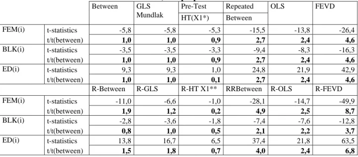
Table 3: t-statistics of time invariant variables, as a proportion of the t-statistics of the between estimator. Pre-Test Repeated Between GLS Mundlak HT(X1*) Between OLS FEVD t-statistics -5,8 -5,8 -5,3 -15,5 -13,8 -26,4 FEM(i) t/t(between) 1,0 1,0 0,9 2,7 2,4 4,6 t-statistics -3,5 -3,5 -3,3 -9,4 -8,3 -16,3 BLK(i) t/t(between) 1,0 1,0 0,9 2,7 2,4 4,6 t-statistics 9,3 9,3 1,0 24,8 21,9 42,9 ED(i) t/t(between) 1,0 1,0 0,1 2,7 2,4 4,6
R-Between R-GLS R-HT X1** RRBetween R-OLS R-FEVD t-statistics -11,0 -6,6 -1,0 -28,1 -14,7 -49,9 FEM(i) t/t(between) 1,9 1,2 0,2 4,9 2,5 8,7 t-statistics -2,8 -3,6 -1,8 -7,4 -7,6 -12,8 BLK(i) t/t(between) 0,8 1,0 0,5 2,1 2,2 3,7 t-statistics 13,8 16,7 6,5 37,4 21,8 63,5 ED(i) t/t(between) 1,5 1,8 0,7 4,0 2,4 6,8
Not for publication:
Table 4: Contribution to R2 in Within regressions with forward selection.
Variable Rank Partial R2 R2
EXP 1 0.6505 0.6505 EXP2 2 0.0060 0.6564 SMSA 3 0.0005 0.6569 UNION 4 0.0004 0.6574 MS 5 0.0002 0.6576 OCC 6 0.0002 0.6578 WKS 7 0.0002 0.6580 IND 8 0.0001 0.6581 SOUTH 9 0.0000 0.6581
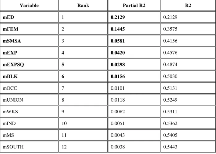
Table 5: Contribution to R2 in Between regressions with forward selection.
Variable Rank Partial R2 R2
mED 1 0.2129 0.2129 mFEM 2 0.1445 0.3575 mSMSA 3 0.0581 0.4156 mEXP 4 0.0420 0.4576 mEXPSQ 5 0.0298 0.4874 mBLK 6 0.0156 0.5030 mOCC 7 0.0101 0.5131 mUNION 8 0.0118 0.5249 mWKS 9 0.0062 0.5311 mIND 10 0.0051 0.5362 mMS 11 0.0043 0.5405 mSOUTH 12 0.0038 0.5443
![[PDF] Cours de base pour créer un document avec Microsoft Word | Formation informatique](data:image/gif;base64,R0lGODlhAQABAIAAAP///wAAACH5BAEAAAAALAAAAAABAAEAAAICRAEAOw==)