Cepstrum-based deconvolution techniques for ultrasonic pulse-echo imaging of flaws in composite laminates

Cepstrum-based Deconvolution Techniques for

Ultrasonic Pulse-echo Imaging of Flaws in

Composite Laminates

Coach K. Wei

Submitted to the Department of Civil and Environmental Engineering

in partial fulfillment of the requirements for the degree of

Master of Science

at the

MASSACHUSETTS INSTITUTE OF TECHNOLOGY

@

Massachusetts

September 1998

Institute of Technology 1998.

All rights reserved.

Author...&

A

u th r

.. . . . .

. . . .. . .. .. .. .. .. . .. . . .. . . ..

2-Department of Civil and Environmental Engineering September 9, 1998

Certified by...

..

Shi-Chang Wooh

Assistant Professor of Civil and Environmental Engineering

,I

ep

f

I )

Thesis Supervisor

A

A ccepted by ... V... . .. -, . ...

Andrew Whittle

0~airman,

MASSACHUSETTS INSTITUTE

Cepstrum-based Deconvolution Techniques for Ultrasonic

Pulse-echo Imaging of Flaws in Composite Laminates

by

Coach K. Wei

Submitted to the Department of Civil and Environmental Engineering on September 9, 1998, in partial fulfillment of the

requirements for the degree of Master of Science

Abstract

Ultrasonic imaging is a powerful nondestructive evaluation (NDE) tool for flaw char-acterization. This thesis discusses the signal processing techniques developed for ultrasonic imaging of flaws in composite laminates. Commonly used time-domain signal processing techniques have problems including poor resolution, dependence on operator's experiences and subjectivity. Some transform-domain processing tech-niques, such as homomorphic deconvolution, eliminate the problems associated with traditional time-domain signal processing techniques. However, these techniques are often sensitive to environmental noise and difficult to apply under certain conditions.

A modified deconvolution technique, based on homomorphic deconvolution, is

pro-posed, which allows for processing real-life signals with noise. Results from inspecting composite laminates show clear improvement of this technique over traditional meth-ods.

Thesis Supervisor: Shi-Chang Wooh

Acknowledgments

My sincere thanks go to Prof. Shi-Chang Wooh, my advisor. His supervision and

guidance through my whole MIT years are the key driving forces that made me reach this point now. In Prof.Wooh's research Lab, NDE Lab, I fully developed my skills in a broad range of areas, such as signal processing, software, system integration and instrumentation. I feel I benefit tremendously from these experiences in my career.

I owe very much to Prof. Daniele Veneziano, my research advisor during the last year at MIT. With his help, I stepped into the area of multifractal iterated random processes and modeling of rainfall. Besides his knowledge, his sense of humor and his kindness to me are all sweet memories I would never forget.

I am also indebted to Prof. Chiang C. Mei, Prof. John R. Williams and Prof.

Srinivas Devadas (Electrical Engineering) and Cynthia Stewart. Their support gave me the courage needed to work through the challenges I had during this journey.

Lots of times I really wish that I would have a chance to show my appreciation to MIT. The campus along Charles River is somehow quite disorganized, but it repre-sents one of the most wonderful places in the world. The two years at MIT will have an enormous influence on my life.

My family and my close friends (Hey, you know your name is in this list) here at

MIT deserve my greatest appreciation. Joys, sweetness, sadness and happiness are all deep in my memory. They added colors to my life here, in fact, lots of colors!

Contents

1 Introduction

1.1 Composite Materials . . . .

1.2 Ultrasonic Nondestructive Evaluation . . . .

1.3 Ultrasonic Imaging Techniques . . . .

1.4 Signal Processing Techniques . . . .

1.5 Motivation and Outline of Thesis . . . .

2 Cepstrum-Based Deconvolution Techniques

2.1 Theory of Homomorphic Deconvolution . . . .

2.1.1 Signal M odel . . . .

2.1.2 Definition of Complex and Real Cepstrum

2.1.3 Homomorphic Deconvolution . . . . 2.2 Sensitivity Study . . . . 2.3 Sum m ary . . . . 8 . . . . 8 . . . . 10 . . . . 13 . . . . 15 . . . . 21 23 . . . . 23 . . . . 24 . . . . 25 . . . . 27 . . . . 31 . . . . 39

3 Modified Techniques for Ultrasonic Pulse-echo NDE of Layered Medium 3.1 Ultrasonic Pulse-echo Signals . . . . 40

3.2 Difficulties in Applying the Homomorphic Deconvolution Technique 44 3.3 Modified Deconvolution Technique . . . . 47

3.4 Sum m ary . . . . 57

4 Ultrasonic Imaging of Composite Laminates 58 4.1 Composite M aterials . . . . 59

Experimental Setup . . Processing of A-Scans Results . . . . Summary . . . .

5 Conclusion and Future Works

4.2 4.3 4.4 4.5 59 60 63 65 69 . . . . . . . . . . . . . . . .

List of Figures

1.1 _{Transducer arrangements: (a) pulse-echo, (b) through-transmission,}

and (c) pitch-catch. . . . . 12

1.2 Ultrasonic scan modes. . . . . 14

1.3 Typical signal processing techniques for B-scan imaging: (a) raw

A-scan signal, (b) rectified signal, (c) video signal, (d) differentiated signal. 16 1.4 Typical A-scan waveforms, gate and threshold setup (Wooh and Daniel,

1994). . . . . 19

1.5 Bscan image resulting from a threshold of 40 (Wooh and Daniel, 1994). 20

1.6 B-scan image resulting from a threshold of 70 (Wooh and Daniel, 1994). 20

1.7 B-scan image resulting from a threshold of 100 (Wooh and Daniel, 1994). 20

2.1 General homomorphic deconvolution procedure. . . . . 28

2.2 An example of homomorphic deconvolution. . . . . 29

2.3 Basic pulse used for signal synthesis (note the deconvolved h(n) is 6(n)). 32

2.4 Deconvolution result when SNR=oo (note h(t) = 6(t) - 0.56(t - 2)).

The artificially introduced time delay between the basic pulse and the

echo, to = 2us, and the scaling factor,ao = -0.5, are both correctly

identified. . . . . 33

2.5 Deconvolution results with different noise level: (a) SNR=1000. (b) SNR=200.

(c) SN R =100. . . . . 35

2.6 Deconvolution results with different number of echoes (SNR=150). (a)

1 echo. (b) 2 echoes. (c) 4 echoes. . . . . 36

2.8 Comparison of the basic pulse and rectangular pulse. . . . .3

3.1 Ultrasonic pulse-echo experiment setup. . . . . 41

3.2 Ultrasonic wave propagation in a typical pulse-echo mode experiment. 42

3.3 Cepstrum-based deconvolution procedure showing a failure in

decon-volving a typical ultrasonic pulse-echo signal . . . . 45

3.4 Deconvolution of the same signal in Fig. 3.3 after lowpass filtering. . 46

3.5 Modified cepstrum-based deconvolution procedure. . . . . 48

3.6 Creating more echoes by taking the absolute value. . . . . 49

3.7 Deconvolution result from the modified deconvolution technique. . . . 50

3.8 Deconvolution result from the traditional deconvolution technique. . . 51 3.9 (a) System for homomorphic deconvolution. (b) Time-domain

repre-sentation of frequency-invariant filtering. . . . . 53

3.10 Time response of frequency-invariant linear systems for deconvolution.

(a) Lowpass system. (b) Highpass system. (Solid line indicates

enve-lope of the sequence 1(t) as it would be applied in a DFT

implementa-tion. The dashed line indicates the periodic extension.) . . . . 53

3.11 False echoes resulted from the modified deconvolution technique. . . . 55 3.12 Post-processing for the modified cepstrum-based deconvolution

tech-nique. . . . . 56

4.1 Schematic of a 16-ply composite laminate with Teflon patches embedded. 60

4.2 Reflection and transmission of ultrasound in material. . . . . 60

4.3 As-obtained waveforms using a transducer with a center frequency of

2.25 MHz and reconstructed signals after deconvolution for a 16-ply [0/ ± 45/90]2, quasi-isotropic graphite/epoxy laminate with embedded

Teflon film patches: (a) Area with no embedded patches, (b) Teflon

patch embedded between the 7 th and 8 th layers, (c) Teflon patch

em-bedded between the 1 1th and 1 2 th layers. . . . . 61

4.4 As-obtained waveforms using a focused transducer with a center fre-quency of 2.5 MHz and reconstructed signals after deconvolution for

a 16-ply [0/ ± 45/90]2, _{quasi-isotropic graphite/epoxy laminate with}

embedded Teflon film patches: (a) Area with no embedded patches,

(b) Teflon patches embedded between the 4 t" and 5th layers, (c)

de-convolution result of the waveform shown in (a), (d) dede-convolution

result of the waveform shown in (b). . . . . 63

4.5 As-obtained waveforms and reconstructed signals after deconvolution for a 12-ply [±152/102], quasi-isotropic graphite/epoxy laminate with real impact damage : (a) Area with no impact, (b) area with impact

damage, (c) Area with impact damage. . . . . 64

4.6 B-scan image of composite laminate with embedded Teflon patch.

Time-dom ain processing. . . . . 66

4.7 B-scan image of composite laminate with embedded Teflon patch.

Mod-ified cepstrum-based deconvolution technique without post-processing. 67

4.8 B-scan image of composite laminate with embedded Teflon patch.

Chapter 1

Introduction

This chapter provides the background of the thesis by an overview of composite materials and ultrasonic imaging. Composite materials are widely used in various structural systems, whose heterogeneous nature and their exposure to various envi-ronments requires new development of nondestructive evaluation (NDE) techniques. This thesis is concerned about using ultrasonics for the inspection of composite ma-terials. Ultrasonics is one of the major NDE techniques, normally operated in either

A-, B- or C-scan mode. However, ultrasonic imaging is gaining wide applications in NDE of composite laminates due to its intuitive way of presenting information.

Com-monly used signal processing techniques in ultrasonic imaging are within the category of time-domain or frequency-domain processing techniques. Their problems include poor resolution, dependence on operator's experiences and subjectivity. These prob-lems bring up the demand for more advanced signal processing techniques. The last section summarizes the whole chapter and gives an outline of the thesis.

1.1

Composite Materials

Composite materials are seeing widespread use throughout aircraft structure systems and air force weapon systems. Recent years they are emerging to be the most signif-icant material for civil engineering infrastructure design and renewal.

A structural composite is a material system consisting of two or more phases on a

macroscopic scale, whose mechanical performance and properties are designed to be superior to those of the constituent materials acting independently. One of the phases is usually discontinuous, stiffer, and stronger and is called reinforcement, whereas the less stiff and weaker phase is continuous and is called matrix. Sometimes, because of chemical interaction or other processing effects, an additional phase, called interphase,

exists between the reinforcement and the matrix. The properties of a composite material depend on the those of the constituents, geometry, and distribution of the phases ( Daniel and Ishai, 1994).

Composites have unique advantages over monolithic materials, such as high strength, high stiffness, long fatigue life, low density, and adaptability to the intended func-tion of the structure. Addifunc-tional improvements can be realized in corrosion resistance, wear resistance, appearance, temperature-dependent behavior, thermal stability, ther-mal insulation, therther-mal conductivity, acoustic insulation. Furthermore, cost for ac-quisition and/or life cycle can be reduced through weight savings, lower tooling costs, reduced number of parts, and fewer assembly operations.

Due to the complexity of composite materials' manufacturing process, quality con-trol during fabrication is essential to guarantee their safe applications. After fabrica-tion, composite structures operate in a variety of thermal and moisture environments that may have a pronounced impact on their performance. These hygrothermal ef-fects are a result of the temperature and moisture content variations and are related to the difference in thermal and hygric properties of the constituents. Service-induced damage growth, such as damage due to impact loading (Daniel and Wooh, 1990; Finn, He and Springer, 1993), must be timely evaluated to prevent potential failure.

Composites present several specific challenges to nondestructive evaluation. Firstly, major defects such as debris, inclusions, delaminations and impact damage must be revealed. Secondly, inspections must reveal defect states such as high void content, fiber bunching, resin richness and ply misorientations. Thirdly, composites need to be evaluated for subtle deficiencies such as those due to diffused flaw populations, microporosity, matrix crazing, fiber breakage, undercure, poor quality fiber/matrix

bonding and poor quality adhesive or interlaminar bonding. Various NDE methods have been used for inspecting composites, including radiographic method, acoustic emission, thermal methods, optical methods, vibration techniques, chemical spec-troscopy, computed tomography, eddy-current testing, ultrasonic methods, electrical and magnetic testing, dielectrometry and microwave techniques. In general, each method displays its advantages and disadvantages over others. Ultrasonic NDE, as a quantitative approach, is of particular interest and also one of the most widely used methods for NDE of composites (Chang, Couchman and Yew, 1971; Wooh and Daniel, 1994).

1.2

Ultrasonic Nondestructive Evaluation

Nondestructive evaluation (NDE) is concerned with identifying, locating and charac-tering structural properties and/or defects in a nondestructive fashion. NDE plays an important role in the life cycle of an engineering structural system (Wooh, 1995). The following list includes the mainstream inspection and monitoring methods currently employed, based primarily on the physical principles of operation:

* Visual/Optical Testing (VT)

" Liquid Penetrant Testing (PT) " Magnetic Particle Inspection (MPI) " Eddy Current (EC)

* Radiographic Testing (RT)

" Acoustic Emission (AE)

" Ultrasonic Testing (UT)

Ultrasound technology is one of the most employed methods for NDE. Ultrasonic waves are mechanical waves oscillating at a frequency beyond 20 kHz, which are

of-material (transducer), generating stress waves which are emitted into an object at fre-quencies in the range of 30 kHz to 50 MHz and higher, depending on the application. Interaction of these waves with the material results in the returning of some por-tion of energy to a receiver, which is further converted into electrical energy through the piezoelectric effect. The signals contain useful information about the inspected material, which could be extracted by using signal processing techniques.

Ultrasonic NDE is widely used for quantitative flaw characterization by deter-mining the location, size and orientation of flaws. In the followings, basic operating modes of ultrasonic testing are introduced first. Then, ultrasonic flaw characteriza-tion methods are discussed. Discussion of ultrasonic imaging techniques is left for the next section for a more detailed description.

Basic Operating Modes

Typically, ultrasonic transducers are set up in one of the three fashions: pulse-echo, through-transmission, and pitch-catch. These techniques are the basic configurations which can lead to more sophisticated modes, as illustrated in Fig. 1.1. A single transducer operating as both transmitter and receiver, as shown in Fig. 1.1(a), emits an ultrasonic signal which is reflected off the backwall of the material and received by the same transducer. This configuration is called pulse-echo, which is often used when inspection is limited to a single side (i.e., single-sided access). If a pair of transducers are placed on opposite sides of the medium, one as a transmitter and the other one as a receiver (Fig. 1.1(b)), the pulse is said to be sent in through-transmission. In the through-transmission mode, transmitter and receiver are physically and electrically isolated, which introduces clean signals and high signal-to-noise ratios. Therefore, this mode is often preferred over pulse-echo, if both sides of the testing material are accessible.

Two transducers situated on the same surface can be used in pitch-catch mode, again in a transmitter-receiver setup, as shown in Fig. 1.1(c). The transmitter sends an oblique beam into the specimen which will be reflected off the opposite side and be caught by the receiver.

test material

(a)

(b).16

Figure 1.1: Transducer arrangements: (a) pulse-echo, (b) through-transmission, and

(c) pitch-catch.

Although the transducers shown in Fig. 1.1 are in direct contact with the solid

through the use of a couplant, all of these methods may easily be extended to

non-contact applications involving a fluid surrounding the specimen.

A-scan

The most fundamental form of information obtained from ultrasonic inspection is

the so-called A-scan, which contains rich information about the material and flaws.

The A-scans are obtained by repetitively transmitting pulses into a material, and synchronizing an oscilloscope to the transmitted bursts. If the transmitting trans-ducer is simultaneously used as a receiver (pulse-echo mode), then the echoes will appear on the screen. The horizontal axis gives time information (this correlates to time-of-flight) while the vertical axis indicates the echo amplitude. Careful analysis

and interpretation of the echoes on the display screen can provide information about

the extent of damage in the material. The A-scan can provide through-thickness information at a point.

Interpretation of the A-scan can lead to quantitative methods to determine cer-tain characteristics, such as its location, size, depth, height, and orientation. This information is critical in assessing the condition of the structure and safeguarding it

experiences and knowledge in NDE. Thus, the need for well-trained personnel who are skilled in calibrating the instrumentation and interpreting signals limits the wide ap-plication of ultrasonic NDE. Ultrasonic imaging exhibits a major improvement here. Presenting information in the form of an image is one of the most intuitive ways to understand, which dramatically reduces the difficulty of data interpretation. This topic will be talked in the next section.

1.3

Ultrasonic Imaging Techniques

Ultrasonic imaging is capable of displaying cross-sectional, planar and full volumetric images of virtually any conceivable material or component using immersion testing. Typically images are categorized into B-scans and C-scans, which are obtained by scanning and processing the A-scans at each point (Krautkimer and Krautkimer,

1990).

B-scan images represent cross-sectional views of defects in the material along a scan line. Using a normal incident ultrasonic beam, a distance between interfaces can be accurately determined by measuring the time interval between the echoes reflected from the interfaces. By processing a series of A-scans along a line of interest and

by mapping the amplitude-time information into pixel information, a cross-sectional

(B-scan) image can be constructed. Figure 1.2 shows schematically the B-scanning procedure.

An image obtained by scanning over an plane is called C-scan, representing a planar view of the material and flaws. In order to provide excellent spatial resolution, a focused transducer is usually used for scanning. In general, intensity or echo ampli-tudes are mapped into brightness of the image while the transducer scans the area of interest on the specimen in a raster fashion, as shown in Fig. 1.2. Since the backface reflection represents the signal loss due to material attenuation and reflection from flaws (if they exist) along the path of ultrasonic wave propagation at each point, gated peak amplitude of backface reflection is often used to construct an image.

A-scan display

B-scan (cross-sectional view)

C-scan (planar image)

...

...

These B- and C- scans are often performed in an immersion tank. Immersion offers several advantages comparing with direct contact testing. An aqueous environment results in the minimum wear of the transducer and forms a uniform and even coupling medium between test material and transducer. Also, the creation of transverse waves due to refraction at the transducer/fluid interface can be avoided since fluids can only sustain longitudinal waves (Krautksmer and Krautkdmer, 1990).

1.4

Signal Processing Techniques

Typically, B-scan and C-scan images are obtained by processing the acquired A-scan waveforms (RF signals) in the time domain. For normal incident pulse-echo mode, the time scale is proportional to the distance from the specimen surface in the thickness direction. Thus, it is possible to map the RF signals into a B-scan image by scanning along a line parallel to the specimen surface. The waveforms acquired during the scanning are interrogated on a point-by-point basis and transformed into a format suitable for B-scan imaging. The as-obtained records have an oscillatory shape whose peaks vary between positive and negative values, as illustrated in Fig. 1.3(a). An image consists of only positive discrete numbers representing gray scale or intensity at a point. Thus, the raw RF signals are not suitable for imaging purposes and some signal processing techniques must be applied.

One simple processing technique is the so-called rectification. This technique maps the absolute values of the RF signal into grayscales, as shown in Fig. 1.3(b). However, this approach is not correct because a single pulse is taken into a series of narrow signals of various amplitudes, as shown in Fig. 1.3(b). A single interface in the material, corresponding to a single pulse in the RF signal, is shown as a series of interfaces with various intensity in the resulting image.

Another processing technique, which is often found in medical diagnostics equip-ment, is illustrated in Fig. 1.3(c). A single pulse is transformed into a video signal

by displaying only the envelope of the positive components. By doing this, a single

im-(b)

(C)

Figure 1.3: Typical signal processing techniques for B-scan imaging: signal, (b) rectified signal, (c) video signal, (d) differentiated signal.

() (d)

(a) raw A-scan

age, which is correct. The disadvantage of this approach is its poor resolution. If the distance between two interfaces are not far enough, the echoes from these interfaces will be mixed together in the RF signal and thus could not be differentiated by this technique.

The other processing technique, which is mostly commonly used in NDE, is by using a gate and setting a threshold. By setting up a gate, which is actually a time window, only the signal inside the gate is processed for imaging and signals outside the window are simply abandoned. Signals whose magnitude smaller than the predetermined threshold value are taken as zero and only those signals whose magnitude exceeds the threshold are mapped into an image. The fourth technique is called differentiated signal, which displays the differentiation of the video signal. This has the advantage of enhancing the amplitude resulting in better reproducible measurements in the time domain. The overall duration of a pulse, however, does not change significantly (Wooh and Daniel, 1994).

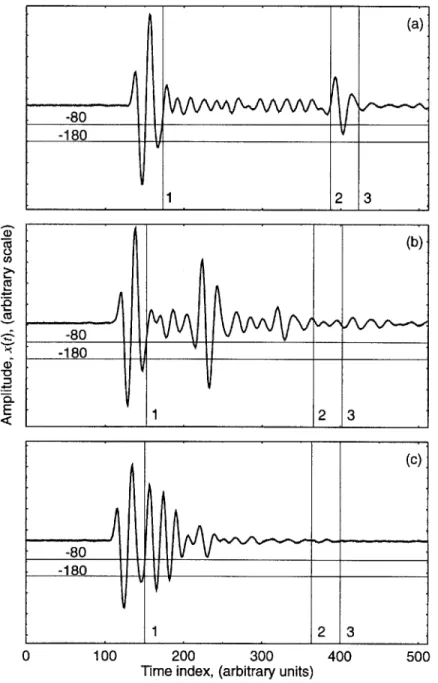
Figure 1.4 shows typical A-scan waveforms and locations of gates and threshold setups. Figure 1.4(a) shows an A-scan in an undamaged region, in which the first echo represents the front face reflection and the one that appears in the gate 2-3 is the backface reflection. Figure 1.4 (b) indicates two delaminations in the middle of the material, one below the other. The latter has a smaller amplitude because of the shadow effect caused by the first delamination. Figure 1.4 (c) shows reflections reflected from a delamination located very close to the front surface. Gate 1-2, which opens at line 1 and closes at line 2, is set to image the cross-section of the material. Gate 2-3, which opens at line 2 and ends at line 3, is used to image the backwall. Two threshold values are chosen: -80 and -180 (arbitrary unit). The problem associated with this method is the subjectiveness in selecting the threshold and gate location. For example, by choosing a threshold of -160, only one delamination is detected in Fig. 1.4(b). Only a threshold around -80 could identify the second delamination correctly. So, a proper selection of the threshold value is the key to successful imaging. There is no theory guiding the selection of threshold value and it is totally dependent on the operator's experience and knowledge in the area. Figures 1.5, 1.6, and 1.7

show the influence of threshold on the image quality. Improper selection of threshold may result in faulty images as shown.

Another problem of this processing technique is its poor resolution. In Fig. 1.4(c), the echoes returned from the front face and the flaw are not separated in the waveform, which means that it is impossible for this time-domain signal processing technique to differentiate the flaw from the frontface. Thus the resolution is limited by the duration of the echo itself, since this technique can only differentiate well-separated echoes.

Drifting of the waveform also causes problems. In general, the waveforms drift back and forth in the time axis at different locations because of surface irregularities or trigger sensitivity of the digitizer. Therefore, for each waveform, the absolute gate opening positions in the array should be calculated by the given relative offset from the front surface reflection rather than by explicitly specified absolute indexes. This adds additional complexity to the hardware system and software system and causes the need for the so-called surface follower mode.

The signals can be also processed in the frequency-domain. One method is to measure the frequency spacing of the resonance peaks in the magnitude spectrum (Chang et al.(1974)). This frequency spacing has a certain relationship with the time-of-flight (TOF) of the echoes and thus the TOF can be determined from the measured frequency spacing. The problem associated with this technique is that it is difficult to automate and requires human interaction. Another technique that has been used by Kinra and Dayal (1988), Iyer and Kinra (1991a, 1991b), Pialucha et al.

(1989) and other researchers is to obtain the spectrum of the system transfer function

and further the TOF information by subtracting the spectrum of the reference pulse from the spectrum of the received waveform. These techniques require an apriori knowledge of the reference pulse and a very stable experimental condition that ensures the repeatability of the reference pulse. Comparing with the time-domain techniques, frequency domain techniques don't require the echoes to be separated in time-domain. But they still have limitations that make their applications difficult in some situations.

(a) -80 __ _ __ _2 -180 1 2 3 (b). -180 2 2 3 (C) --180 12 3 0 100 200 300

Time index, (arbitrary units)

400 500

Figure 1.4: Typical A-scan waveforms, gate and threshold setup (Wooh and Daniel, 1994).

CO

0

It,

Figure 1.5: Bscan image resulting from a threshold of 40 (Wooh and Daniel, 1994).

Figure 1.6: B-scan image resulting from a threshold of 70 (Wooh and Daniel, 1994).

In summary, while processing A-scan waveforms could result in B-scan or C-scan images, which are much more intuitive for flaw detection, all the above processing techniques have some serious drawbacks. The signal processing technique to enhance the quality of ultrasonic images remains an ongoing research topic.

1.5

Motivation and Outline of Thesis

Ultrasonic NDE is a powerful technique for flaw characterization in many applications. The basic modes of operation are: pulse-echo, through-transmission, and pitch-catch.

By using these methods, it is possible to determine the size, location and orientation

of flaws by processing the obtained A-scan waveforms. Data interpretation here is crucial for the successful application of ultrasonic NDE.

However, sufficient experiences and knowledge in NDE is required for data in-terpretation. The need of well-trained personnel for operation somehow limits the application of ultrasonic NDE. In this sense, ultrasonic imaging provides a much more intuitive way for presenting information. Grayscale or color images can be eas-ily used to determine size, location and orientation of flaws, which may reduce the need of skilled personnel.

B-scan and C-scan are mostly used imaging methods. The first provides an image of a cross-section while the latter provides a planar view of the material. They are obtained through scanning and processing of the obtained A-scan waveforms.

The current implementations are mostly based on time-domain processing. While they have been successfully applied, they have many drawbacks. The resolution is limited by the duration of the echo; the selection of time window (gate) is subjec-tive; the choice of amplitude threshold is also subjective. Frequency-domain signal processing techniques offer some comparative advantages. But they require either human interaction, apriori knowledge or stable testing conditions. The existence of these problems necessitates the need for new and robust signal processing techniques. This thesis is targeted for the research on this problem.

The thesis will first introduce a useful echo detection technique, homomorphic deconvolution. This technique gives good result if the signal is free from noise. But the sensitivity of this technique hinders its application in ultrasonic imaging. After a sensitivity analysis of homomorphic deconvolution, a modified cepstrum-based de-convolution technique is proposed. This technique overcomes the extreme sensitivity to noise and makes using deconvolution techniques for ultrasonic imagine feasible. Following the discussion of this proposed technique, an application of the technique to ultrasonic imaging of composite laminates is presented. Conclusion and future works are presented in the last chapter.

Chapter 2

Cepstrum-Based Deconvolution

Techniques

This chapter provides the basic theory of cepstrum-based deconvolution techniques.

Homomorphic deconvolution, an excellent solution for some of the signal processing

problems in ultrasonic NDE, is introduced first. The major mode of difficulties in applying this theory resides in its sensitivity to noise. To this end, a sensitivity study based on numerical experiments is performed. Unfortunately, in ultrasonic

NDE, most of the signals contain certain level of noise due to various reasons, which

deters the application of this deconvolution technique. The study in this chapter is the foundation for the proposed signal processing technique for ultrasonic pulse-echo imaging, which will be discussed in the next chapter.

2.1

Theory of Homomorphic Deconvolution

The concept of cepstrum was introduced by a paper titled The Quefrency Analysis

of Time Series for Echoes: Cepstrum, Pseudoautocovariance, Cross-Cepstrum and Saphe Cracking by Bogert, Healy and Tukey (1963). They observed that the

loga-rithms of the power spectrum of a signal containing an echo has an additive periodic component due to the echo, and thus the Fourier transform of the logarithm of the power spectrum should exhibit a peak at the echo delay. They called this function the

cepstrum. At about the same time, Oppenheim (1969) proposed a new class of

sys-tems called homomorphic syssys-tems. The transformation of a signal into its cepstrum is a homomorphic transformation. Since then, the concepts of the cepstrum and homomorphic systems have proved useful in signal analysis and have been applied with success in speech signal processing (Oppenheim, 1969; Schafer and Rabiner,

1970), seismic signals (Ulrych, 1971; Tribolet, 1979), biomedical signals (Senmoto

and Childers, 1972) and sonar signals (Reut et al., 1985). Here we will introduce the theory and its possible application in ultrasonic NDE.

2.1.1

Signal Model

Assume y(t) is the signal under investigation and furthermore we assume that y(t) is a convolution of two components, x(t) and h(t). In other words, we consider our

signal model to be:

y(t) = x(t) * h(t) , (2.1)

in which h(t) is the impulse response function of the system. We assume h(t) is composed of a series of spikes that could be approximated as

N

h(t) =

(

i=O

where 6(t) is a delta function:

00, t=0 6(t)=

0, otherwise

This is a typical echo-detection model, which simply says y(t) is composed of x(t) and its echoes. This kind of model is very useful and widely seen in the aforementioned signal processing areas. We will show that this model can also be applied to the

both unknown. But we know that h(t) is composed of a series of spikes, as expressed

by eq. (2.2). The question is how to obtain h(t), which is our point of interest. If we

take y(t) as the output of the system, and x(t) as the input, then h(t) is the response function of the system. The problem is how to obtain the system function while only the output known. In other words, we are interested in deconvolving x(t) and h(t) so that we could obtain h(t). This is a deconvolution problem.

Today signals are mostly processed in the discrete-time domain. Typically, a continuous analog signal, say x(t), is sampled at a period of T, the so-called sampling

period, and quantized at a resolution of 8 to 16 bits. Considering discretization, the

signal is modeled equivalently as:

y(n) = x(n) * h(n) , (2.3)

where n is the time index and the time t = nT. Similarly, h(n) is the corresponding

impulse response function of the system, which is assumed to be a series of spikes approximated as

N-1

h(n) = ai6(n - ni) . (2.4)

i=0

For the sake of simplicity, we will take this discrete signal model as our basic model in the following discussions.

2.1.2

Definition of Complex and Real Cepstrum

Suppose X(w) is the Fourier transform of a stable signal x(t), X(w) could be ex-pressed in polar form as:

where

IX(w)|

number X(w), w is the frequency and

j

root of -1.

The complex cepstrum of x(n) is defined to be a stable signal t(n) whose Fourier transform is

X(w) = log[X(w)]. (2.6)

Normally the natural logarithm is used, which will be assumed throughout this thesis, although any base could be used for the logarithm. The logarithm of a complex number X(w) is defined as:

log[X(w)] = log[IX(w)|] + jarg(X(w)) . (2.7)

However, the imaginary part of eq. (2.7) is not well defined yet since the angle for complex number is only unique within integer multiples of 27. For further discussion of this definition, refer to Oppenheim and Schafer (1991). Some important properties of complex cepstrum are outlined as follows:

" Property 1: The complex cepstrum decays at least as fast as 1

|nl

" Property 2: t(n) will have infinite duration, even if x(t) has finite duration. " Property 3: If x(n) is real, then ±(n) is also real.

Besides the complex cepstrum, the real cepstrum c,,(n) is defined as the inverse transform of the logarithms of the magnitude of the Fourier transform:

The relationship between the real cepstrum cr(n) and the complex cepstrum 2(n) can be shown as:

c (n) = 2 . (2.9)

Compared to the real cepstrum, the complex cepstrum reserves all the information and original signal x(n) could be fully recovered from the complex cepstrum. But the complex cepstrum is much more difficult to compute, since it involves not only the magnitude of the Fourier transform but also the angle. The real cepstrum is, on the other side, easier to compute but it is not invertible.

2.1.3

Homomorphic Deconvolution

For a system of input x(n) and output y(n) such as

y(n) = x(n) * h(n) ,

Fourier transform of the above equation can be written as:

Y(w) = X(w)H(w) , (2.10)

where Y(w), X(w), and H(w) are the respective frequency representations of y(n),

x(n), and h(n). As a result, convolution in the time domain becomes multiplication

in the frequency domain. By further taking a logarithm operation of eq. (2.10), we obtain:

log[Y(w)] = log[X(w)] + log[H(w)] . (2.11)

Taking an inverse Fourier transform, the following equation relating the complex ceptra 9(n), t(n), and hI(n) holds:

y(t) logo: 18 -- IFFT

"Frequency

I

E

Invariant

Filtering

h(t)

+

IFFT

exp() -T

FFT

Figure 2.1: General homomorphic deconvolution procedure.

Now we are in the so-called quefrency domain. Suppose t(n) and h(n) are sepa-rable in this domain, we could remove t(n) from 9(n), and then obtain the complex cepstrum of h(n) and correspondingly recover h(n).

Extraction of h(n) from

g(n)

frequency-invariant filtering, in which h(n) is approximately taken as (for simplicity, we will use

' =' _{in the following equation instead of} '' ):

h(n)

where l(n) is a frequency-invariant filter. Suppose that t(n) = 0 for n > no and

h(n) = 0 for n < no, then a frequency-invariant linear filter such as

0, for n <no

l(n) =

1, for n > no

will remove t(n) from 9(n) and thus recover h(n).

The problem in question is whether 2t(n) and h(n) are separable. Theory shows

1

that, according to Property 1, zt(n) decays at least as fast as . So most of the

3 2 1 0 -1 (b). Fourier Transform -2' 0 1 2 Time(second) (c).Cepstrum -0.5 0 3 4 x 10-6 2 4 6 8 10 12 Frequency(Hz) (d).Reconstructed h(n) 0.4 0.2 0 -0.2 -0.4 0.5 1 1.5 Quefrency(second) X 10-5 1 2 Time(second) 3 14 x 106 4 x 106

Figure 2.2: An example of homomorphic deconvolution.

around zero in the quefrency domain. On the other hand, it could also be shown that

h(n), if h(n) has the expression of eq. (2.2), will stand out in the area away from 0 in

the quefrency domain. The different characteristics of the two kinds of signals make the separation in the quefrency domain possible.

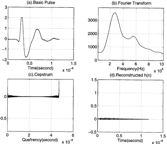
After extracting h(n) from 9(n), h(n) can be reconstructed from hI(n) by taking the inverse of the operations done so far. In summary, the homomorphic deconvolution procedure is shown in Fig. 2.1. An example of using this technique to deconvolve a signal is shown in Fig. 2.2. Figure 2.2(a) to 2.2(d) respectively show the as-obtained waveform, the magnitude of Fourier transform, the real cepstrum of the signal and the

deconvolved signal h(n). An echo located at t = 2 pus is clearly and precisely identified

-

...

-- -. .. ...-. ..-. .-. ..-. ..-.

..--hlM M

-- - --

-.-.

in the deconvovled signal. Also, the echo has a negative polarity and its amplitude is approximately 0.3 according to h(n). In the deconvolution, a frequency-invariant high-pass filter was used.

2.2

Sensitivity Study

This section introduces numerical studies of the cepstrum-based homorphic deconvo-lution. As shown in the example in the previous section, this technique seems to be an excellent tool that deconvolves signals blindly. It is shown in Fig. 2.2 that the time-of-flight of the echo can be precisely and clearly identified. However, this deconvolution technique is very sensitive to noise. In application to ultrasonic pulse-echo signals, this technique failed for most of the signals we aquired. To understand the possible factors influencing the deconvolution result, a sensitivity study is executed based on numerical experiments. According to the need in ultrasonic signal processing, the following three factors are considered in the numerical studies:

" Signal-to-noise Ratio(SNR) " Bandwidth

" Number of echoes contained in the signal

In the following experiments, all the signals used are artificially synthesized by using a basic pulse, x(n). This basic pulse is truncated from an ulrasonic pulse-echo experimental waveform. The shape of the pulse and its spectrum are shown in Fig. 2.3. Each signal, denoted by y(n), which is actually used for the numerical experiment, is synthesized by scaling the basic pulse, namely multiplying x(n) by a constant ai (-1 < ao < 1), shifting the scaled basic pulse by a certain time delay t

t-(or, using time index, ni = , T is the sampling period). This scaled and shifted

pulse is denoted by aix(n - _{ni). This procedure may be repeated several times to}

create several echoes. The signal y(n) is obtained by adding together the basic pulse

x(n) and these shifted and scaled versions, aix(n - ni), i = 0, ..., N - 1. Following

this procedure, we get

N-1

h(n) = Z ajo(n - ni),

i=O

(b). Fourier Transform 0.5 1 1.5 2 4 6 8 10 Time(second) X 10-6 Frequency(Hz) X 106 6 (d). Reconstructed h(n) 1.5 0 .5 - - -..- -. 0 -. 5.-.-.- . -0.5 0 0.5 1.5 x 106 (c).Cepstrum -0.5 4 Quefrency(second) X 10-6 1 Time(second)

Figure 2.3: Basic pulse used for signal synthesis (note the deconvolved h(n) is 6(n)).

0 2

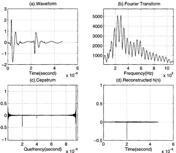
(b).Fourier Transform 2 4 6 Time(second) X 10-6 (c).Cepstrum 2 4 6 8 10 Frequency(Hz) X 10 (d).Reconstructed h(n) 1 0 .5 -. . ... . .... ... . 0-- 0 .5 -. -. . . ... . . .-..-..-.- .. . ..-.-_ 1 ... ... ... .1 - 0 .5 1 2 4 6 8 0 2 4 6 Quefrency(second) X 10-6 Time(second) X 10

Figure 2.4: Deconvolution result when SNR=oo (note h(t) = 6(t) - 0.56(t - 2)). The

artificially introduced time delay between the basic pulse and the echo, to = 2us, and

the scaling factor,ao = -0.5, are both correctly identified.

Signal-to-Noise Ratio

Figure 2.4 shows the deconvolution result when SNR-+ oo (i.e., no additive noise). The synthesized signal, y(t), is obtained by adding up the basic pulse and a scaled, shifted version of the basic pulse, with a scaling factor of -0.5 and a time delay

of 2 ps. This implies that h(t) = 6(t) - 0.56(t - 2). The signal-to-noise ratio is

considered to be oc, since no noise is introduced due to the fact that y(t) is precisely

modeled by y(t) = x(t) * h(t) with h(t) = 6(t) - 0.56(t - 2). The deconvolution

result is almost perfect in the sense that the acquired h(n) matches the theoretical

h(t) = 6(t) - 0.56(t - 2) extremely well. 1

0.5

0

The result shown in Fig. 2.4 seems to indicate great promise of applying this deconvolution technique to real experimental data. However, a further study, by adding random white noise to synthesized signals, shows extreme sensitivity of the technique to noise. Figure 2.5 shows the effect of increasing noise level. Signals used in this figure are similar to those used in Fig. 2.4, except for having a certain amount of white noise added. They are generated using the following formula, where x(t) is the basic pulse:

y(t) = x(t) - 0.5x(t - 2) + #w(t) ,

which implies h(t) = 6(t) - 0.56(t - 2) as in Fig. 2.4. The only difference is the

inclusion of the additive noise,

#w(t).

between -1 and 1. The parameter

#

The signal-to-noise ratio (SNR) is defined as the ratio between the maximum value

of the basic pulse x(t) and the maximum of the additive noise

#w(t).

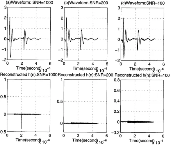
SNR of 1000, 200 and 100 are used for signals (a), (b) and (c), respectively. The simulated signals are shown on the top of the figures while the deconvolved results

are shown at the bottom of the figures. For SNR = _{1000, deconvolution still gives a}

very good estimation of h(t), as shown in Fig. 2.5 (a). The time delay of the echo is precisely identified but the estimation of the scaling factor, ao, is slightly degraded,

compared to SNR = oc in Fig. 2.4. With a SNR = 200, in Fig. 2.5 (b), the time

delay is still correctly identified but the estimation of the scaling factor, ao, is further

degenerated. When the noise level is raised to a SNR = 100, the estimation of h(t)

from deconvolution is close to a failure, as shown in Fig. 2.5 (c).

Although homomorphic deconvolution gives excellent echo detection when the signal is clean, it fails with even a very low noise level. In Fig. 2.5 (c), noise is only one percent of the signal and the signal does not look much degraded from that of Fig. 2.5(a). The failure of homomorphic deconvolution in this case implies the extreme sensitivity of this technique. Unfortunately, it is likely that most of the ultrasonic pulse-echo signals have at least this amount of noise, which deters the direct

(a)Waveform: SNR=1000 (b)Waveform:SNR=200 3 3 2 - 2 -- .-.- .- .- . -.-. -. 1 ... 1.. ... .. .... .. 0-- 0---. ... --2 -2 0 2 4 6 0 2 4 6 Time(second) 10-6 Time(secon) 10-6 Reconstructed h(n):SNR=1 000 Reconstructed h(n):SNR=200 1 1 0 .5 - - .-- .-.---- .---0 .5 ---... 0 --- .. . 0 -0.5 (c)Waveform:SNR=100 3 2 01 -2 0 2 4 6 Time(secon) 10-Reconstructed h(n):SNR=100 0.8 0.6 ---0.4 ---0 .2 -. -.--0 0 2 4 6 0 2 4 6 0 2 4 6

Time(secon) 10-6 Time(seconQ 10-6 Time(second)

10-Figure 2.5: _{Deconvolution results with different noise level: (a) SNR=1000.}

(b) SNR=200. (c) SNR=100.

-(a)1 echo 3 0 -2' 0 5 10 15 Time (us) Reconstructed h(n):1 Echo 0.5 0.4 -0.3 0.2 0.1 - - -0 -0.1 0 5 10 15 Time (us) (b)2 echoes Time (us) Reconstructed h(n): 2 Echoes 0.5 0 .4 -... -- -0.3 - - -0.2 -0 .1 - - - - . 0 -0.1 -0 5 10 15 Time (us) (c)4 echoes 3 0 -1 -2 0 5 10 15 Time (us) Reconstructed h(n): 4 Echoes 0.5 0.4 --0 .3 . -. - .. -.-. -.-. -0.2 - -0.1 -0 0.1 0 5 10 15 Time (us)

Figure 2.6: Deconvolution results with different number of echoes (SNR=150). (a) 1 echo. (b) 2 echoes. (c) 4 echoes.

application of this technique to echo detection. This also explains partially why this technique is still not widely used for ultrasonic signal processing even though it has the ability to give a perfect echo detection.

Number of Echoes

Figure 2.6 shows the effect of increasing the number of echoes. At the same noise level, the more echoes the signal contains, the better the deconvolution result will be. This has some practical implication in ultrasonic pulse-echo signal processing.

By capturing a longer waveform, which could contain more echoes than a shorter

waveform, better results are expected. However, a longer waveform requires more processing time and storage. Thus the trade-off should be well measured.

(a)SNR=100, Narrow-band Signal

0 2 4 6 8

Time (us)

econstructed h(n): Narrow-band Signal

0 2 4 Time (us) 6 8 3 2 1 0 -1 -2 0 2 4 6 8 Time (us)

Reconstructed h(n): Broad-band Signal

1h I 0.5 0 -0.5' 0 2 4 Time (us) 6 8

Figure 2.7: Deconvolution results: effect of bandwidth.

Bandwidth

To investigate the effect of the bandwidth of the basic pulse, two signals are synthesized. The first signal, shown in Fig. 2.7 (a), is obtained by convolving the

basic pulse x(t) with h(t) = 6(t) - 0.956(t - _{2us). The second signal is obtained by}

replacing the basic signal with a rectangular pulse, as shown in Fig. 2.7 (b). The same amount of additive noise, with a SNR= 100, is added to both signals. Deconvolution results are shown in Fig. 2.7 (c) and (d). Deconvolving the first signal barely reveals the structure of h(t) while h(t) is clearly identified in the second case.

A comparison of the two pulses are shown in Fig. 2.8. The difference lies in the

fact that a rectangular pulse has a much broader bandwidth than the basic pulse. This accounts for the difference in the deconvolution results.

0.8 0.6 0.4 0.2 0 -0.2 ... ... ... (b)SNR=100, Broad-band Signal -. . . . ... -. ...- -- - - ... -- . .- - -. .... ... ..- -- 10-I R

(c)Rectangular Pulse 5U 400-300 200 100 0 0 Time (us)

(b).Fourier Transform of Basic Pulse

20 40 60 80

Frequency (MHz)

Figure 2.8: Comparison of the

Time (us)

(d).Fourier Transform of Rectangular Pulse

50 4 0 - -. -- .-. -30 -.-20 - - -.- .-10 -- - -. - . -0 0 20 40 60 80 Frequency (MHz)

basic pulse and rectangular pulse.

3 . . . . . . . . ... . . . . ' ' (a)Basic Pulse

As a conclusion, this deconvolution technique works better with broadband sig-nals compared to narrow band sigsig-nals. As a guideline for application, broadband transducers are preferred to narrow band transducers.

2.3

Summary

In summary of the above numerical studies, the following conclusions are drawn:

" When the signal is clean, cepstrum-based deconvolution technique is capable of

providing perfect estimation of h(t) without knowing x(t).

" This technique is very sensitive to noise. It could fail even with very low noise

level.

* Incorporating more echoes into the signal gives better deconvolution result.

" The cepstrum-based deconvolution technique performs better over broad band

signals compared with narrow banded ones, which suggests a preference on broadband transducers.

These conclusions give insight into this signal processing technique and useful hints for experiments. Homomorphic deconvolution, although has good echo detection capability when the signal is clean , is too sensitive to noise to be applied to deconvolve real ultrasonic signals. Based on the above conclusions, a modified cepstrum-based deconvolution technique is proposed. This modified deconvolution technique is based on homomorphic deconvolution we discussed in this chapter, but it is more robust so that the noise contained in real experimental data doesn't cause failure to the application of the algorithm. It makes deconvolution of real ultrasonic experimental data feasible. Details of this modified deconvolution technique will be the topic of the next chapter.

Chapter 3

Modified Techniques for Ultrasonic

Pulse-echo NDE of Layered

Medium

This chapter discusses an ultrasonic pulse-echo detection model and proposes a sig-nal processing technique based on traditiosig-nal homomorphic deconvolution techniques. Due to the noise level in experimental data, traditional deconvolution techniques often fail in application. A modified deconvolution technique is proposed to address this issue. Experiments show that this modified cepstrum-based deconvolution technique works well in practice. Also, a post-processing technique to eliminate the by-product of the modified cepstrum-based deconvolution technique is suggested. Sample appli-cations are demonstrated.

3.1

_{Ultrasonic Pulse-echo Signals}

A typical ultrasonic pulse-echo setup is shown in Fig. 3.1. An ultrasonic transducer

is used both as a transmitter and a receiver, either in contact or non-contact. In immersion testing, water is used as a coupling medium. The received waveform, which usually includes a main bang, and echoes from the front face, internal interfaces

Figure 3.1: Ultrasonic pulse-echo experiment setup.

about the testing material. It is usually displayed on an oscilloscope and may be further digitized and stored in a host computer.

In brief, a received waveform, denoted by y(t), can be modeled as the convolution of x(t), frontface reflection of the ultrasonic pulse generated by the transducer, and the system function, h(t). As a function of the testing material, h(t) contains all the relative information about the material. We are interested in the investigation of the material, which normally involves estimating a part of or the complete h(t):

y(t) = x(t) * h(t) , (3.1)

where h(t) is expressed in general as

N

h(t) =

(

i=0

A multi-layer model is illustrated in Fig. 3.2, in which a testing sample is assumed

to be of several layers immersed in water. Layer 1 is made of material 1, with a

thickness of hi, a wave speed of c1. Likewise layer 2 is made of material 2, with a

thickness of h2 and a wave speed of c2, and so on. An ultrasonic pulse emitted from the

transducer propagates into water first and then hits the interfaces between the layers: interface 1 (the interface between water and material 1); interface 2 (the interface

Incident Reflected wave waves xQ) x(t) x,(t) x,(t) interface 1I

i

Figure 3.2: Ultrasonic wave propagation in a typical pulse-echo mode experiment.

between material 1 and material 2); interface 3 (the interface between material 2 and the material below material 2). Reflection coefficients, denoted by R,, are shown in the figure, where x represents the material that ultrasound comes from and y represents the material that ultrasound propagates into. For example, Roi represents the reflection coefficient when the wave is propagating from water into material 1.

RIO denotes the reflection coefficient as the wave is propagating from material 1 into

water. Similarly, Transmission coefficients donated by Txy are defined in a similar

fashion. For instance, T12 represents the transmission coefficient of the amount of

wave transmitting into materials 2 from material 1 and T21 represents the transmission

coefficient in case that wave is propagating into material 1 from material 2, and so on.

A pulse generated by the transducer is denoted by xo(t). Similarly, x(t) denotes

the first reflection of xo(t) from interface 1, x1(t) represents the first reflection of

xo(t) from interface 2 and x₂(t) represents the first reflection of xo(t) from interface

3, which can be expressed for one-dimensional waves as:

H

_ _ _ _2

Material

I

R₂₁,T₂₁

h2,c2

x0(t 2ho) Co R12T1Oxo(t - 2h 2h₁) Co C1 T12R 23T21T1Oxo(t - 2h0 Co 2h, 2h₂ 1 2

)

Solving for xo(t) from x(t) and then substituting the corresponding result into the

expressions of x, (t) and x2(t), we get:

X1() ToiR12To 2hi X1(t) = x(t - ) x2() = x(t--x3(t) =---ToiR 12Tio a1 = _Ro ToiT12R23T21To a2 = 2hi Cl 2h,1 t2 = -C]

Equation (3.1) can be rewritten as:

x1(t)

x2(t)

x3(t)

+ 2h2

C₂

The received signal can be written as:

y(t) = x(t) + x1(t) + x2(t) + x3(t) + x(t) = Ro1 x1(t) = To1 x₂(t) =TO1 x3(t) =-

-I

)

Substituting x1(t) = aix(t - ti) and x2(t) = a2x(t - t2) into eq. (3.3), we get eq. (3.4):

y(t) = x(t) + aix(t - ti) + a2x(t - t2) + , (3.4)

which can be rewritten as:

y(t) = x(t) * h(t) , (3.5)

where:

h(t) = 6(t) + a16(t - t1) + a26(t - t2) + - (3.6)

In short, the received signal is a convolution of the front face reflection and a function h(t), which is a simple function but contains all the information we are interested, such as wave speed, reflection coefficients, transmission coefficients, etc. We may define h(t) as the system function. More precisely, it is the system impulse

response function. In general, x(t) is not limited to be the frontface reflection but

from any interface. It is also possible to incorporate material attenuation in the model in a similar fashion.

As we know, the pulse-echo waveform contains rich both amplitude information and time-of-flight information. The above model, based on 1-D wave equations, gives insight into the relationship between the as-obtained waveform and material properties and thus lays the foundation for ultrasonic pulse-echo signal processing.

3.2

_{Difficulties in Applying the Homomorphic}

De-convolution Technique

As shown in Chapter 2, cepstrum-based deconvolution is capable of fully recov-ering h(t) from y(t) without knowing x(t). To this end, the cepstrum-based

decon-(b). Fourier Transform ...... ...--....- ....-. ..-. ...- . -. ...- .-250 200 150 100 50 2 4 6 8 Time(second) (c).Cepstrum x 10-6 5 10 15 Quefrency(second) 5 10 Frequency(Hz) (d).Reconstructed h(n) 15 x 106 0 .6 --. . . -. --.-.. ---. . -.-. . -.- -. --0 .4 - . . . . .. . .. . .. . . .-.. . . . . . 0.2 0 0 2 4 6 8 x 10-6 Time(second) x 106

Figure 3.3: Cepstrum-based deconvolution procedure showing a failure in deconvolv-ing a typical ultrasonic pulse-echo signal.

21 - 0--1 -2 -0 0.4 0.2 0 -0.2 -0.4 (a).Waveform