HAL Id: hal-01935322
https://hal.archives-ouvertes.fr/hal-01935322
Submitted on 26 Nov 2018
HAL is a multi-disciplinary open access
archive for the deposit and dissemination of
sci-entific research documents, whether they are
pub-lished or not. The documents may come from
teaching and research institutions in France or
abroad, or from public or private research centers.
L’archive ouverte pluridisciplinaire HAL, est
destinée au dépôt et à la diffusion de documents
scientifiques de niveau recherche, publiés ou non,
émanant des établissements d’enseignement et de
recherche français ou étrangers, des laboratoires
publics ou privés.
Experimental Validation of a Multirobot Distributed
Receding Horizon Motion Planning Approach
José Mendes Filho, Eric Lucet, David Filliat
To cite this version:
José Mendes Filho, Eric Lucet, David Filliat. Experimental Validation of a Multirobot Distributed
Receding Horizon Motion Planning Approach. ICARCV 2018 - 15th International Conference on
Control, Automation, Robotics and Vision, Nov 2018, Singapour, Singapore. �hal-01935322�
Experimental Validation of a Multirobot Distributed Receding Horizon
Motion Planning Approach
Jos´e M. Mendes Filho
a, b, ∗, Eric Lucet
aand David Filliat
bAbstract— This paper addresses the problem of motion planning for a multirobot system in a partially known environment where conditions such as uncertainty about robots’ positions and communication delays are real. In particular, we detail the use of a Distributed Receding Horizon Approach that guarantees collision avoidance with static obstacles and between robots communicating with each other. Underlying optimization problems are solved by using a Sequential Least Squares Programming algorithm. Experiments with real nonholonomic mobile platforms are performed. The proposed framework is compared with the Dynamic Window approach to motion planning in a single robot setup. A second experiment shows results for a multirobot case using two robots where collision is avoided even in presence of significant localization uncertainties.
I. INTRODUCTION
A Multirobot System (MRS) is a system composed by multiple robots operating in the same environment. These systems have received a great deal of interest for their potential to accomplish complicated tasks in different application domains such as exploration [1], [2], transportation [3], [4], construction [5] and more.
An indispensable capability for MRS is Motion Planning (MP). MP can be broadly defined as the problem of generating a collision-free trajectory (sequence of poses and velocities) from an initial to a final pose. Although simple in its definition, this problem is PSPACE-hard [6]. For the past decades, many approximate approaches to solve this problem have been proposed [7], [8]. It remains, though, a major focus of robotics, especially when robots’ workspaces are dynamic partially known environments - in which case the problem is shown to be intractable (NP-hard) [9]. Furthermore, far less work has been carried out for addressing the MP problem for MRS than for single robot systems, as pointed out in [10].
An increasingly common approach for addressing this problem is the use of mathematical programming. It offers flexibility to explicitly accommodate multiple systems requirements simultaneously. In most cases, these requirements are a subset of the following list: kinematics, dynamics, collision avoidance and connectivity maintenance requirements [11].
Our previous work presented in [12] fits this group of mathematical programming methods by proposing a formulation of the MRS MP problem as distributed nonlinear
aCEA, LIST, Interactive Robotics Laboratory, Gif-sur-Yvette, F-91191,
France
b U2IS, ENSTA ParisTech, Inria FLOWERS team, Universit´e
Paris-Saclay, 828 bd des Mar´echaux, 91762 Palaiseau cedex France
∗corresponding author:[email protected]
programming problems (NLPs) solved by each robot in the system. It then interleaves planning and execution in the partially known environment by using a Receding Horizon approach. It aims to generate dynamically feasible and collision-free trajectories for a MRS composed of nonholonomic ground vehicles modeled as unicycle-type robots. NLPs are numerically solved by using a Sequential Least Squares Programming algorithm (SLSQP) [13], [14]. The complete approach is referred to as DRHMP (Distributed Receding Horizon Motion Planning).
This paper builds on that work with three main objectives: i) to discuss strategies and implementation techniques in order to use the DRHMP approach in real mobile robots; ii) to compare the DRHMP to another MP approach for a single robot system; iii) to demonstrate the robustness of the DRHMP in presence of localization and tracking errors and real communication conditions between two robots.
In order to accomplish those objectives, the DRHMP approach was implemented on two Turtlebots 2 platforms [15] equipped with rangefinder sensors (structured-light 3D scanners). Its performance was compared with that of a Dynamic Window approach (DWA) used by default in the ROS navigation stack.
The paper is thus organized as follows: the next section gives a brief summary of related work on MRS MP, Section III provides a presentation of the DRHMP approach. In Section IV the experimental setup for verifying that approach is detailed along with the most significant contributions of this work. The last two sections present results and conclusions.
II. RELATED WORK
Approaches for solving the MRS MP problem can be classified in many different ways. Refer to [16], [10] for comprehensive surveys on the subject. Here we aim only to review a few recent works that closely relate to ours.
In [17] a mathematical programming and distributed receding horizon approach is used for MRS MP. Robots are required to communicate and exchange their current and most recent states. That information is used to predict robots trajectories assuming uniform linear motion. Then, those predictions are used to form collision avoidance constraints in the optimization problem. An interesting aspect of this approach is that it splits the planning horizon into two parts: during the first part collision avoidance and smoothness of trajectories are dealt with; in the second part only global target convergence is a concern. An incremental
sequential convex programming (iSCP) algorithm for solving the optimization problems is used. Only results in simulation are shown.
Work presented in [18] proposes a Decentralized Nonlinear Model Predictive Control (DNMPC) for addressing MRS MP where careful convergence and feasibility analysis are provided. Formation maintenance, avoidance of static obstacles and inter-robot collision avoidance are verified in simulation for unicycle robots but the approach could be generalized for other types of systems. The method requires though that the robots communicate sequentially and it is not clear how the underlying finite horizon optimization control problems for each robot are solved. This approach too remains to be tested in a real experiment.
Another recent relevant work on Distributed MPC for MRS is presented in [19]. Instead of relying on complete predictions of other robots trajectories it uses occupancy grid data aiming for a reduction in the required communication means. The approach was tested on nonholonomic mobile platforms using an external motion capture system for localization of the mobile platforms.
Our approach closely relates to the one presented in [17]. The main differences consist in how collision constraints are handled and how localization and tracking errors are modeled. In [17] the problem of having non-differentiable constraints for obstacle avoidance is addressed by transforming them into smooth nonlinear constraints. Conversely, our work derives differentiable smooth constraints from sampled data (inflated occupancy grids given by the perception module) by doing local interpolations around sampled points in robots’ planned trajectories. As for localization and tracking errors, [17] assumes they are always inferior to a small constant while our work uses a probabilistic model and confidence regions to produce robust collision-free trajectories.
III. DISTRIBUTEDRECEDINGHORIZONMOTION PLANING
In the DRHMP approach, each robot in the MRS computes its own local trajectory. Analogous to a MPC, a prediction time-horizon Tpand a computation timeslot Tc are defined1. Tp is the time-horizon for which a local solution to the motion problem will be computed and Tc is the timeslot during which a portion of that solution is implemented while the next plan - created for the next time-horizon Tp- is being computed.
For each receding horizon planning problem, the following two steps are performed:
Step 1: Each robot computes its own intended solution trajectory by solving a constrained nonlinear optimization problem (NLP). In that problem all needed constraints are
1The term receding horizon is favored over the more used term MPC [20]
because the DRHMP uses more than just the first element of the optimal solution for computing the system’s input. In other words, since Tcis usually
greater than the lower level controller time period Tt, the first Tc/Ttelements
of the solution are implemented.
included except coupling constraints, meaning constraints that involve solving a conflict between multiple robots such as collision or loss of communication. The solution found at this step is referred to as step1-generated trajectory.
Step 2: Robots involved in a potential conflict (risk of collision, or communication loss) update their trajectories computed at Step 1 by solving a second NLP that additionally takes coupling constraints into account. For evaluating those additional coupling constraints the robots asynchronously exchange their step1-generated trajectories. If a robot is not involved in any conflict, its step2-generated trajectory becomes equal to the one found at Step 1 avoiding solving the second NLP.
When a robot arrives closer to its goal, a termination procedure for reaching the goal is used. It takes the desired final configuration as a hard constraint in the optimization problem and uses the time for reaching the goal as the cost function to be minimized. Refer to works [12], [21] for more details.
An example of the resulting receding horizon optimization problem solved at Step 2 for a given robot R can be written as follows: min q(t)kq(τk+ Tp) − qgoalk, ∀t ∈ [τk, τk+ Tp] (1) subject to: ˙ q(t) = f (q(t), u(t)), ∀t ∈ [τk, τk+ Tp] q(τk) = q(τk−1+ Tc) ˙ q(τk) = ˙q(τk−1+ Tc) v2(t) ≤ v2 max, ∀t ∈ (τk, τk+ Tp] ω2(t) ≤ ωmax2 , ∀t ∈ (τk, τk+ Tp] a2(t) ≤ a2max, ∀t ∈ [τk, τk+ Tp] α2(t) ≤ αmax2 , ∀t ∈ [τk, τk+ Tp]
d(O,t) ≥ εo, ∀t ∈ (τk, τk+ Tp], ∀O ∈O d(Rc,t) ≥ εr(Rc), ∀t ∈ (τk, τk+ Tp], ∀Rc∈C d(Rd,t) ≤ min(dcom, dd,com), ∀t ∈ (τk, τk+ Tp], ∀Rd∈D with τkthe starting discrete time for the kth receding horizon optimization problem, f the kinematic model of the robot, q= (x, y, ψ) the vehicle’s pose, u the system’s input, v = k[ ˙x ˙y]k, ω = ˙ψ , a = k[ ¨xy]k, α = ¨¨ ψ , O the set of obstacles known by robot R at τk−1,C the set of collision candidates vehicles for robot R at τk−1, D the set of communication loss candidates for robot R at τk−1, dcom the maximum communication range of robot R, dd,com the maximum communication range of robot Rd, εothe minimum distance allowed between robot R and any obstacle, and εr(Rc) the minimum distance allowed between robots R and Rc.
In our previous work, when applying this approach, several assumptions about communication, perception and magnitude of different errors were made that do not hold in a real application.
First, when testing in simulation, computations of each robot were made by a different thread under a unique process. This allowed the use of shared memory for communicating among virtual robots which could be considered instantaneous within that context.
Another unrealistic assumption was about perception. Once an obstacle entered the perception range of a vehicle, a perfect knowledge of that obstacle’s shape (polygon or circle) and pose was considered. It was possible then to solve simple algebraic expressions for computing the distance from a given point to the obstacle.
Finally, localization of simulated robots was precise and accurate and tracking errors were reasonably small. That allowed for the use of constant, small tolerance values for constraints concerning collision avoidance (i.e. constant, small εo and εr).
IV. EXPERIMENT SETUP
This section details how each of the unrealistic assumption presented above - concerning communication, perception and errors - were compensated for in order to use the DRHMP in a real experiment. Two Turtlebots 2 [15] mobile robots were used for such purpose.
A. MRS architecture
The DRHMP approach was implemented as a plugin (named codrha local planner) adhering to the BaseLocalPlannerinterface provided by the nav core ROS package. This allows for using other features already present in the ROS navigation stack [22] such as occupancy grids, global planners, etc.
Each robot launched its own ROS master node and all other nodes needed for navigation, including an instance of codrha local planner.
Communication between robots was conducted outside ROS systems for messaging (typically Topics or Services). Specific socket programming was implemented so exchange of information among robots could be as minimal as possible. A mobile ad-hoc network (MANET) over Wi-fi (IEEE 802.11) was used. Ad-hoc networks represent a more robust architecture compared to infrastructure mode networks (which use central Access Point) and more flexible, scalable and cheap than architectures with fixed topology in general [23].
The embedded computers on each robot had a dual core Intelr Celeronr N3060 @ 1.60GHz CPU. For better performance, priority and affinity configurations of threads had to be set properly. Communication-related threads were set with affinity to one of the cores (e.g. core 0) with higher priority than any other processes in the system (e.g. priority 10). In turn, all ROS-related threads were launched with affinity to the remaining core (e.g. core 1) with priority only lower than communication-related threads (e.g. priority 9).
Time synchronization among robots is a critical aspect of any MRS. In the DRHMP the need of a common global time is fundamental to the evaluation of conflict between vehicles. In a wireless network, the problem becomes even more challenging due to the possibility of collision of the synchronization packets on the wireless medium and the higher drift rate of clocks on the low-cost wireless devices. In this experiment, time synchronization was achieved by using an alternative NTP client and server called chrony [24],
designed for systems that are not permanently online. It is supposed to provide an accuracy typically in the tens of microseconds.
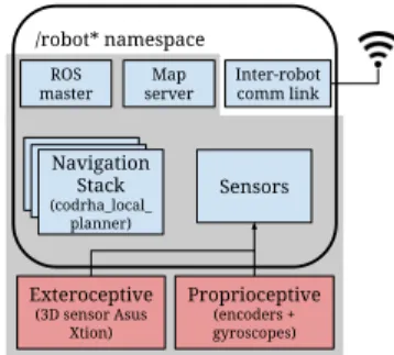
An architecture representing the most relevant components of a robot in the MRS can be seen in Fig. 1.
/robot* namespace Navigation Stack (codrha_local_ planner) Sensors Exteroceptive (3D sensor Asus Xtion) Proprioceptive (encoders + gyroscopes) ROS master Map server Inter-robot comm link
Fig. 1: Overview of a robot composing the MRS
B. Localization and tracking error compensation
Localization for vehicles used in the experiments was done by using a particle filter [25] merging data from gyroscopes, encoders, rangefinder sensors and static map. As well as for any localization system, there is inherent error associated with the robot’s estimated configuration. That uncertainty can be characterized by the covariance matrix of the robot’s configuration which is known for each robot at each instant τk. Likewise, each robot can estimate its tracking error based on the planned reference trajectory and its configuration estimate.
Both covariation values and tracking error were sent as part of the information exchanged between robots along with their estimated configuration and planned trajectory. This enables a given robot R to compute a conservative “safety distance” from robot Rc that is time dependent and can replace the constant εr(Rc) in the NLP constraints.
The new value is computed according to the equation: εr(Rc,t) = εtr(t) + εloc(t) + εtr, Rc(t) + εloc, Rc(t) (2)
where εtr is simply the euclidean norm of lateral and longitudinal tracking errors and εloc is a confidence value related to position estimates. εloc depends on the covariance matrix given by the robots’ localization modules, and its expression is given by Eq. 3:
εloc(t) = q
χv2(2)kλ0, λ1k∞ (3) with λ0and λ1being the eigenvalues of the covariance matrix associated with the bivariate normal distribution of possible locations in the XY plane of a robot at an instant τk. χv2(2) is the 2 degrees of freedom chi-square value for a (1 − v) confidence region (CR).2
Similarly, εo in the NLP constraints can be replaced by εo(t), where:
εo(t) = εtr(t) + εloc(t) (4) Fig. 2 shows a graphical representation of errors εtr(t) and εloc(t) at instant τk.
2A 95% CR (i.e. χ2
Fig. 2: Localization and tracking errors representation. The 95% Confidence Region ellipse encompasses the central 95% of the probability mass of possible locations for a robot at instant τk. The ellipse is dilated by the robot’s radius.
C. Use of costmap for obstacle avoidance
Instead of a complete geometric description of obstacles as used in previous works [12], [21], only 2D costmaps are available for the purpose of obstacle avoidance when using ROS navigation stack. These costmaps are based on occupancy grids generated from 3D sensor data and user defined inflation radius that is meant to take the robot’s footprint into account.
Directly using those costmaps for computing obstacle avoidance constraints in the DRHMP is not straightforward. The solution that worked best can be described in two steps. First, the occupancy grid is inflated according to a linear function that goes from the highest possible cost value at an occupied position in the grid, to zero at a position located at a distance equals to the radius of the robot.
Secondly, bicubic interpolations of the costmap around sample points taken along a trajectory candidate are performed. Those interpolations provide a locally defined, continuous and differentiable distance function for each sample during optimization. A representation of this approach for one sample is displayed in the Fig. 3.
The importance of having a continuous differentiable distance functions comes from the way the SLSQP solver searches for a solution: it uses finite differences to estimate first and second order derivatives of constraints. Without interpolations, those finite differences would usually evaluate to zero. That is because the differentiation step size h employed by SLSQP is much smaller than the occupancy grid resolution.
V. RESULTS
Experiments were carried out in order to investigate two aspects: how the DRHMP compares to another local MP in a “single robot avoiding an obstacle” situation and how well collision avoidance between two robots running the DRHMP is performed in face of real communication, perception and trajectory tracking issues. Across all experiments we used vmax = 0.2 m/s, amax = 0.5 m/s2, Tp= 3.8 s, Tc = 0.3 s. A simple controller designed for tracking a reference admissible trajectory based on the kinematic model of the system was used [26].
A. Experiment 1 - Single robot obstacle avoidance
A testbed as shown in Fig. 4 was used for comparing collision avoidance with a static obstacle using the
Fig. 3: 3D representation of the costmap and local interpolation used by the codrha local planner. Cost values of 254 correspond to the detected surface of an obstacle
DRHMP approach and the well known Dynamic Window approach (DWA) [27]. Although admittedly each planners’ performance can be highly impacted by the configuration of its parameters, an effort was made to set those values so equivalent behaviors could be obtained. Velocity and acceleration limitations were set to same values for instance.
(a) (b)
Fig. 4: Experiment 1. (a) shows a representation of the testbed using the same map information as the localization system of the real robots. (b) is an actual photo of the testbed
As indicated in Fig. 4 the “robot” located near the XY origin had to reach the “target” point located about 2.3 m of its initial position. An obstacle of about 20 cm in diameter not known by the robot in advance was placed in the way.
Table I summarizes the performance of each planner regarding five criteria. Mean and standard deviation (Std) data were based on 10 trials for each algorithm.
TABLE I: Experiment 1 summary
DRHMP DWA
Mean Std Mean Std travel time (s) 12.637 0.084 18.790 0.385 average linear speed (m/s) 0.193 0.000 0.136 0.002 final position error (m) 0.014 0.004 0.092 0.013 final yaw error (rad) 0.011 0.004 0.355 0.053 min clearance from obstacles (m) 0.069 0.014 0.228 0.023
In none of the tests neither MP approaches failed to avoid obstacles. Compared to DWA, DRHMP can be seen as a less conservative approach. It keeps less clearance from obstacles and can produce a higher average linear velocity in order to minimize travel time. That behavior derives from the type of objective function used in the NLPs. Similarly, DWA’s behavior derives from its scoring algorithm. It worth noticing that DRHMP presents an inferior standard deviation compared to DWA which suggests it is a more stable approach. Typical paths adopted by both algorithms can be seen in Fig. 4a.
B. Experiment 2 - Multirobot motion planning
Experiment 2 consisted of having two robots going successively from one target location in their shared workspace to another. Those targets positions were such that the robots would execute two different triangle-shaped loops that share a common side. Along this shared side the two robots (if the timing was right) would have to cross each other to reach their next target. The robots’ trajectories in Fig. 5 illustrate this setup.
For better evaluating the DRHMP performance in that scenario two different sub-experiments were set. In sub-experiment 2a a simplification about tracking and localization errors was made. They were considered equal to zero by the DRHMP algorithm running in both robots (εr= 0). It implied though that the physical robots had to be kept still during planning to prevent them from colliding. As we will see, the εr= 0 assumption is far from realistic, provided the platforms we worked with. Sub-experiment 2b, on the contrary, makes no such simplification and εris based on the real information about the physical robots executing the planned trajectories. This second case shows how even with errors of about 50 cm the DRHMP can safely find collision-free trajectories for both physical robots.
Everything else, specially communication is done in the same way across both experiments.
1) Sub-experiment 2a:
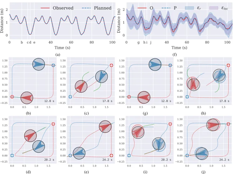
The trajectories produced and the inter-robot distance along this entire sub-experiment can be seen in Figs. 5a to 5e. Planned trajectories would allow both robots to avoid each other with almost no clearance at four different moments as indicated by the inter-robot distance curve passing near zero in Fig. 5a.
Figs. 5b to 5e represent four snapshots of both robots planning processes around the first moment of collision avoidance. The green continuous lines in front of the robots represent the XY points of their planned trajectory for the horizon Tp(i.e. step2-generated trajectories). The dashed line in front of a given robot Rarepresents what the other robot Rb thinks Ra will do (i.e. Ra’s step1-generated trajectory as known by Rbas a result of their communication).
When collision is not an issue, dashed lines may superpose almost exactly the green continuous ones3. In contrast, as collision becomes an issue, one can observe a greater
3communication delays may still prevent them from being identical
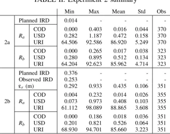
TABLE II: Experiment 2 summary
Min Max Mean Std Obs Planned IRD 0.014 - - - -COD 0.000 0.403 0.016 0.044 370 Ra USD 0.282 1.187 0.472 0.158 370 2a URI 64.506 92.586 86.920 5.249 370 COD 0.000 0.265 0.017 0.038 323 Rb USD 0.280 0.895 0.512 0.134 323 URI 64.204 92.623 85.962 4.714 323 Planned IRD 0.376 - - - -Observed IRD 0.253 - - - -εr (m) 0.292 0.933 0.435 0.106 351 COD 0.004 0.232 0.014 0.026 355 2b Ra USD 0.073 0.973 0.408 0.103 355 URI 61.112 98.089 88.865 3.608 355 COD 0.000 0.186 0.018 0.036 351 Rb USD 0.201 0.821 0.526 0.064 351 URI 68.930 94.701 85.660 3.223 351 RI = received information
URI = % of the RI that is actually used by the DRHMP at Step 2 COD = communication delay measured by the receiving end in seconds USD = delay between receiving and start using RI in DRHMP in seconds IRD = inter-robot distance in meters
difference between those two types of trajectories. At Fig. 5c, Ra’s step1-generated trajectory as known by Rb is shown as coming straight at Rb. Ra’s step2-generated trajectory, in green, is quite different from that and clearly avoids a future collision. That is because Ra has already taken into account Rb’s step1-generated trajectory into its Step 2.
Following the time sequence and observing Fig. 5d, one can see that the actually followed paths after solving the conflict reflect a smaller deviation from the otherwise straight-line trajectory when compared to those planned green lines in Fig. 5c. This is due to the Receding Horizon nature of the approach which interleaves planning and execution and therefore reconsiders the avoidance trajectory adapting to the changes made by the other robot. Its implication, albeit conditioned to Tc values, is that collision avoidance ends up being achieved with near the minimum clearance possible (zero in this case). Furthermore, a natural compromise between robots is achieved: they both deform their initial straight trajectories of comparable amounts.
That is precisely the behavior expected for the DRHMP in a multirobot scenario and observed in simulation in previous works [12].
2) Sub-experiment 2b:
In this sub-experiment the physical robots actually did navigate their workspace and the real observed information about their localization and trajectory tracking was used in the DRHMP.
Due to imprecision of sensors, actuators and low level controllers, εr becomes meaningful in this second case as shown by the error bands in Fig. 5f. That has the effect of reducing the space of acceptable solutions in which the DRHMP searches for optimal trajectories. If, additionally, the workspace is very cluttered there may be no acceptable solutions left yielding optimization errors at the SLSQP algorithm level.
(a) (b) (c) (d) (e) (f) (g) (h) (i) (j)
Fig. 5: Experiment 2 results. (a) to (e) refer to sub-experiment 2a while (f) to (j) to sub-experiment 2b. “Planned” or “P” data shows inter-root distance computed based on the planned trajectories generated by the DRHMP approach. “Observed” or “O” data represents the same distance but based on observed/estimated actual position of the robots. In (f) the blue and purple error bands centered around the “Planned” line represent respectively the safety distance of Eq. 2 (εr) and its localization component (εloc,Ra+ εloc,Rb).
Nevertheless, for the studied setup, acceptable solutions were always found and the inter-robot collision of the physical robots were prevented at all times throughout the experiment (as observed in the experiment video in [28]).
From Fig. 5g to 5j the difference between black and colored circles representing the robots reflects the tracking error. Black circles use the mean information of robots’ localization systems while colored ones use the planned poses. As before, dashed and green continuous lines in front of a given robot represent respectively the step1-generated trajectory known by the other robot and its own step2-generated trajectory.
The utility of a nonconstant εr taking robots localization uncertainty into account can be appreciated in Fig. 5f. It can be observed that when εr takes smaller values (such as near time 45s compared to time 20s) the inter-robot distance can be reduced as well.
Table II summarize statistics of experiment 2 regarding communication and inter-robot distances. Comparing
communication-related values between robots Ra and Rb and then between sub-experiments 2a and 2b shows indeed that communication conditions where very symmetric. The column titled “Obs” shows the number of observations and it is roughly equal to the duration of the experiment divided by Tc(the period the robots exchange step1-generate trajectories). Furthermore, due to the asynchronism between robots’ planning processes and to communication delays, it is common that part of the trajectory information received by a robot concerns a time interval of no interest to that robot. In other words, at Step 2 of the DRHMP the information about another robot’s trajectory may be partially too old or planned for too far into the future. The percentage of the information that can actually be used is referred to as URI. Overall, despite considerable communication delays (tens of ms), low quality localization (main responsible for high εr values) and use of a simple kinematic controller that does not take sliding and actuator response times into account, the DRHMP manages to produce satisfying results with respect
to multirobot collision avoidance. VI. CONCLUSIONS
In this paper, a Distributed Receding Horizon Motion Planning approach for Multirobot Systems is presented and tested in real experiments. We detail its implementation on two mobile platforms as a mean of discussing solutions for dealing with real application limitations concerning communication and perception. Its performance is compared with the Dynamic Window approach in a single robot setup. Tests for multirobot system are also carried out showing the robustness of the DRHMP in presence of localization uncertainties and real communication delays.
Among the future research directions that could be explored based on this work, we particularly think that a generalization of the approach for different systems (not only unicycle-like vehicles) for supporting non-homogeneous multi-robot systems is of great interest and relatively straightforward.
Moreover, in this work we assume that robots can obtain information about other robots by directly communicating with them (as in a fully connected topology). This is an unrealistic assumption for robots in a mobile ad-hoc network where topology is dynamic and self-organizing. The use of an efficient and secure distributed ledger [29] for sharing information among all robots in the network would be an interesting improvement and enable tests with a greater number of robots without prohibitively increasing communication requirements.
REFERENCES
[1] W. Burgard, M. Moors, C. Stachniss, and F. E. Schneider, “Coordinated multi-robot exploration,” IEEE Transactions on robotics, vol. 21, no. 3, pp. 376–386, 2005.
[2] T. Nestmeyer, P. R. Giordano, H. H. B¨ulthoff, and A. Franchi, “Decentralized simultaneous multi-target exploration using a connected network of multiple robots,” Autonomous Robots, vol. 41, no. 4, pp. 989–1011, 2017.
[3] I. Maza, K. Kondak, M. Bernard, and A. Ollero, “Multi-uav cooperation and control for load transportation and deployment,” in Selected papers from the 2nd International Symposium on UAVs, Reno, Nevada, USA June 8–10, 2009. Springer, 2009, pp. 417–449. [4] C. Amato, G. Konidaris, G. Cruz, C. A. Maynor, J. P. How, and
L. P. Kaelbling, “Planning for decentralized control of multiple robots under uncertainty,” in Robotics and Automation (ICRA), 2015 IEEE International Conference on. IEEE, 2015, pp. 1241–1248. [5] F. Augugliaro, S. Lupashin, M. Hamer, C. Male, M. Hehn,
M. W. Mueller, J. S. Willmann, F. Gramazio, M. Kohler, and R. D’Andrea, “The flight assembled architecture installation: Cooperative construction with flying machines,” IEEE Control Systems, vol. 34, no. 4, pp. 46–64, 2014.
[6] J. Hopcroft, J. Schwartz, and M. Sharir, “On the complexity of motion planning for multiple independent objects; pspace- hardness of the “warehouseman’s problem”,” The International Journal of Robotics Research, vol. 3, no. 4, pp. 76–88, 1984. [Online]. Available: https://doi.org/10.1177/027836498400300405
[7] H. Choset, K. M. Lynch, S. Hutchinson, G. A. Kantor, W. Burgard, L. E. Kavraki, and S. Thrun, Principles of Robot Motion: Theory, Algorithms, and Implementations. Cambridge, MA: MIT Press, June 2005.
[8] S. M. LaValle, Planning Algorithms. New York, NY, USA: Cambridge University Press, 2006.
[9] J. Canny and J. Reif, “New lower bound techniques for robot motion planning problems,” in Foundations of Computer Science, 1987., 28th Annual Symposium on. IEEE, 1987, pp. 49–60.
[10] M. Mohanan and A. Salgoankar, “A survey of robotic motion planning in dynamic environments,” Robotics and Autonomous Systems, vol. 100, pp. 171 – 185, 2018. [Online]. Available: http://www.sciencedirect.com/science/article/pii/S0921889017300313 [11] P. Abichandani, G. Ford, H. Y. Benson, and M. Kam, “Mathematical
programming for multi-vehicle motion planning problems,” in 2012 IEEE International Conference on Robotics and Automation, May 2012, pp. 3315–3322.
[12] J. M. Mendes Filho, E. Lucet, and D. Filliat, “Real-Time Distributed Receding Horizon Motion Planning and Control for Mobile Multi-Robot Dynamic Systems,” in ICRA 2017-IEEE International Conference on Robotics and Automation, 2017.
[13] D. Kraft, “A software package for sequential quadratic programming, Tech. Rep. 28, 1988.
[14] S. G. Johnson, “The NLopt nonlinear-optimization package.” [Online]. Available: https://nlopt.readthedocs.io/en/latest/
[15] “TurtleBot2 - Open-source robot development kit for apps on wheels,” http://www.turtlebot.com/turtlebot2/, accessed: 2018-01-23.
[16] M. Hoy, A. S. Matveev, and A. V. Savkin, “Algorithms for collision-free navigation of mobile robots in complex cluttered environments: A survey,” Robotica, vol. 33, no. 3, pp. 463–497, 2015.
[17] Y. Zhou, H. Hu, Y. Liu, S. W. Lin, and Z. Ding, “A Real-Time and Fully Distributed Approach to Motion Planning for Multirobot Systems,” IEEE Transactions on Systems, Man, and Cybernetics: Systems, vol. PP, no. 99, pp. 1–15, 2017.
[18] A. Filotheou, A. Nikou, and D. V. Dimarogonas, “Robust decentralized navigation of multi-agent systems with collision avoidance and connectivity maintenance using model predictive controllers,” arXiv preprint arXiv:1804.09039, 2018.
[19] M. W. Mehrez, T. Sprodowski, K. Worthmann, G. K. Mann, R. G. Gosine, J. K. Sagawa, and J. Pannek, “Occupancy grid based distributed mpc for mobile robots,” in Intelligent Robots and Systems (IROS), 2017 IEEE/RSJ International Conference on. IEEE, 2017, pp. 4842–4847.
[20] L. Grne and J. Pannek, Nonlinear model predictive control: theory and algorithms. Springer Publishing Company, Incorporated, 2013. [21] J. M. Mendes Filho and E. Lucet, “Multi-Robot Motion Planning: a Modified Receding Horizon Approach for Reaching Goal States,” Acta Polytechnica, vol. 56, no. 1, pp. 10–17, 2016. [Online]. Available: https://ojs.cvut.cz/ojs/index.php/ap/article/view/3440/3334 [22] “ROS 2D navigation stack,” http://wiki.ros.org/navigation, accessed:
2018-02-27.
[23] S. Giordano et al., “Mobile ad hoc networks,” Handbook of wireless networks and mobile computing, pp. 325–346, 2002.
[24] “Chrony - an alternative NTP client and server,” https://chrony. tuxfamily.org/, accessed: 2018-05-02.
[25] S. Thrun, W. Burgard, and D. Fox, Probabilistic robotics. MIT Press, 2005.
[26] B. Siciliano and O. Khatib, Springer handbook of robotics. Springer Science & Business Media, 2008.
[27] D. Fox, W. Burgard, and S. Thrun, “The dynamic window approach to collision avoidance,” IEEE Robotics and Automation Magazine, vol. 4, no. 1, pp. 23–33, 1997.
[28] J. M. Mendes Filho, E. Lucet, and D. Filliat. Distributed Receding Horizon Motion Planning for Multirobot Systems. Youtube. [Online]. Available: https://youtu.be/bpxKhNzhJU8
[29] E. C. Ferrer, “The blockchain: a new framework for robotic swarm systems,” CoRR, vol. abs/1608.00695, 2016. [Online]. Available: http://arxiv.org/abs/1608.00695