HAL Id: hal-00741970
https://hal.inria.fr/hal-00741970
Submitted on 15 Oct 2012
HAL is a multi-disciplinary open access archive for the deposit and dissemination of sci-entific research documents, whether they are pub-lished or not. The documents may come from teaching and research institutions in France or abroad, or from public or private research centers.
L’archive ouverte pluridisciplinaire HAL, est destinée au dépôt et à la diffusion de documents scientifiques de niveau recherche, publiés ou non, émanant des établissements d’enseignement et de recherche français ou étrangers, des laboratoires publics ou privés.
Distributed computing of efficient routing schemes in
generalized chordal graphs
Nicolas Nisse, Ivan Rapaport, Karol Suchan
To cite this version:
Nicolas Nisse, Ivan Rapaport, Karol Suchan. Distributed computing of efficient routing schemes in generalized chordal graphs. Theoretical Computer Science, Elsevier, 2012, 444 (27), pp.17-27. �hal-00741970�
Distributed computing of efficient routing schemes
in generalized chordal graphs
∗Nicolas Nisse1
, Ivan Rapaport2
and Karol Suchan3,4
1
MASCOTTE, INRIA, I3S, CNRS, UNS, Sophia Antipolis, France.
2
DIM, CMM (UMI 2807 CNRS), Universidad de Chile, Santiago, Chile.
3
Facultad de Ingenier´ıa y Ciencias, Universidad Adolfo Ib´a˜nez, Santiago, Chile.
4
WMS, AGH - University of Science and Technology, Cracow, Poland.
Abstract
Efficient algorithms for computing routing tables should take advantage of the particular properties arising in large scale networks. Two of them are of particular interest: low (logarithmic) diameter and high clustering coefficient.
High clustering coefficient implies the existence of few large induced cycles. Considering this fact, we propose here a routing scheme that computes short routes in the class of k-chordal graphs, i.e., graphs with no induced cycles of length more than k. In the class of k-chordal graphs, our routing scheme achieves an additive stretch of at most k − 1, i.e., for all pairs of nodes, the length of the route never exceeds their distance plus k − 1.
In order to compute the routing tables of any n-node graph with diameter D we propose a distributed algorithm which uses messages of size O(log n) and takes O(D) time. The corresponding routing scheme achieves the stretch of k − 1 on k-chordal graphs. We then propose a routing scheme that achieves a better additive stretch of 1 in chordal graphs (notice that chordal graphs are 3-chordal graphs). In this case, the distributed computation of the routing tables takes O(min{∆D, n}) time, where ∆ is the maximum degree of the graph. Our routing schemes use addresses of size log n bits and local memory of size 2(d − 1) log n bits per node of degree d.
Keywords: Routing scheme, stretch, chordal graph, distributed algorithm.
1
Introduction
In any distributed communication network it is important to deliver messages between pairs of processors. Routing schemes are employed for this purpose. A routing scheme is a distributed algorithm that directs traffic in a network. More precisely, any source node must be able to route messages to any destination node, given the destination’s network identifier. When investigating routing schemes, several complexity measures arise. On the one hand, it is desirable to use as short paths as possible for routing messages. Efficiency of a routing scheme is measured in terms of its multiplicative stretch factor (resp., additive stretch factor), i.e., the maximum ratio (resp., difference) between the length of a route computed by the scheme and that of a shortest path connecting the same pair of nodes. On the other hand, as the amount of storage at each
∗Partially supported by programs of Conicyt Chile: Anillo ACT88 (K.S.), Basal-CMM (I.R. and K.S.), Fonde-cyt 1090156 (I.R.), FondeFonde-cyt 11090390 (K.S.), Instituto Milenio ICDB (I.R.) and the European Commission through the EULER project (Grant No.258307) part of the Future Internet Research and Experimentation (FIRE) objective of the Seventh Framework Programme (FP7). (N.N.).
processor is limited, the routing information stored in the processors’ local memory (the routing tables) must not require too much space with respect to the size of the network. Last but not least, because of the dynamic character of networks, it is important to be able to compute the routing information in an efficient distributed way. While many works propose good tradeoffs between the stretch and the size of routing tables, the algorithms that compute those tables are often impracticable because they are centralized or because of their time-complexity. Indeed, in the context of large scale networks like social networks or Internet, even polynomial time algorithms are inefficient. In this paper, we focus on the tradeoff between the length of the computed routes and the time complexity of computing the routing tables. In the distributed model we consider, the ”time” refers to the number of rounds in which O(log n)-bit messages are exchanged between nodes (local computations are ”instantaneous”).
One way to design efficient algorithms in large scale networks consists in taking advantage of their specific properties. In particular, they are known to have low (logarithmic) diameter and to have high clustering coefficient. Therefore, their chordality (the length of the longest induced cycle) is somehow limited (e.g., see [Fra05]). That is why, in this paper, we focus on the class of k-chordal graphs. A graph G is called k-chordal if it does not contain induced cycles longer than k. A 3-chordal graph is simply called chordal. This class of graphs received particular interest in the context of compact routing. Dourisboure and Gavoille proposed routing tables of at most log3
n/ log log n bits per node, computable in time O(m + n log2
n), that give a routing scheme with additive stretch 2⌊k/2⌋ in the class of k-chordal graphs [DG02]. Also, Dourisboure proposed routing tables computable in polynomial time, of at most log2n bits, but that give an additive stretch k + 1 [Dou05]. Using a Lexicographic Breadth-First Search (Lex-BFS) ordering (resp., BFS-ordering) of the vertices, Dragan designed a O(n2
)-time algorithm to approximate the distance between all pairs of nodes up to an additive constant of 1 in n-node chordal graphs, and up to k − 1 in, more general, k-chordal graphs [Dra05]. All these time complexity results consider the centralized model of computation.
In this paper we propose a simpler routing scheme which, in particular, can be quickly computed in a distributed way and achieves good additive stretch for k-chordal graphs. However, the simplicity comes at a price of O(log n) bits per port needed to store the routing tables. Distributed Model. An interconnection network is modeled by a simple, undirected, con-nected n-node graph G = (V, E). In the following, D denotes the diameter of G and ∆ denotes its maximum degree. The processors (nodes) are autonomous computing entities with distinct identifiers of size log n bits. We consider an all-port, full-duplex, O(log n)-bit messages, syn-chronous communication model. That is, links are bidirectional, so, in one communication step, each processor is able to simultaneously send and receive different messages of size O(log n) to and from, respectively, each of its neighbors. By results of Awerbuch and Peleg [AP90], our algorithms can be adopted to asynchronous networks at a cost of a polylogarithmic overhead. As usual in the context of distributed computation, the time-complexity of algorithms is defined by the required number of communication steps.
Our results. We present a simple routing scheme using a relabeling of the vertices based on particular BFS-trees. Using a Strong-BFS-tree1
(see Section 2 for the definition), our algorithm achieves an additive stretch k − 1 in the class of k-chordal graphs, and using a Maximum Neighborhood BFS-tree (Max-BFS-tree), it achieves an additive stretch 1 in the class of chordal graphs. It uses addresses of size log n bits and local memory of size 2(d − 1) log n bits per node
1
The name BFS-tree is often used in distributed computing literature to denote any shortest paths tree. To emphasize the particular properties of BFS-trees that are used in this work, the authors decided to add the prefix “Strong” in the name, even though the BFS-trees found in textbooks on algorithms usually are Strong-BFS-trees in this sense.
of degree d. More precisely, each node must store an interval (two numbers, i.e., 2 log n bits) per port, for all except one port.
The stretches which we achieve are equal to the best ones obtained in previous works. But our algorithm is a (simple) distributed one. It uses O(log n)-bit messages. It computes a relabeling of the vertices and the routing tables in time O(D) when a Strong-BFS-tree is used, and in time O(min{∆D, n}) when a Max-BFS-tree is used. Note that this time-complexity corresponds to the number of communication steps.
In the class of chordal graphs, our results simplify those of Dragan since a Lex-BFS-ordering is more constrained than a Max-BFS-ordering. In particular, the design of a distributed algo-rithm that computes a Lex-BFS-ordering of the vertices of any n-node graph G in time o(n) is an open problem even if G has small diameter and maximum degree.
Related work. Two kinds of routing schemes have been studied. In the name-independent model, the designer of the routing scheme has no control over the node names (see, e.g., [PU89, GP96, GG01]). Here we focus on labeled routing, where the designer of the routing scheme is free to name the nodes with labels containing some information about the topology of the network, the location of the nodes in the network, etc. In this context, a routing scheme with multiplicative stretch 4k − 5, k ≥ 2, and using ˜O(n1/k
) bits per node2
in arbitrary graphs is designed in [TZ01]. In the case of trees, optimal labeled routing schemes using ˜O(1) bits per node have been proposed in [FG01, TZ01]. In [FG01], it is shown that any optimal routing scheme using addresses of log n bits requires Ω(√n) bits of local memory. Several network classes have been studied, like planar graphs [Tho04], graphs with bounded doubling dimension [AGGM06], graphs excluding a minor [AG06], etc.
A particular labeled routing scheme is interval routing. Defined in [SK85], interval routing has received particular interest [Gav00]. In such a scheme, the nodes of the network are labeled using integers, and outgoing arcs in a node are labeled with a set of intervals. The set of intervals associated to all the outgoing edges of a node forms a partition of the name range. The routing scheme consists in sending the message through the unique outgoing arc labeled by an interval containing the destination’s label. The complexity measure is the maximum number of intervals used in the label of an outgoing arc. An asymptotically tight complexity of n/4 intervals per arc in an n-node network is given in [GP99]. Moreover, almost all networks support an optimal interval routing scheme using at most 3 intervals per outgoing link [GP01]. Specific graph classes have been studied in this context (e.g., bounded treewidth graphs [NN98]).
2
Generalities on BFS-orderings and BFS-trees
In the following, G = (V, E) denotes a connected n-node graph. Let H = (V (H), E(H)) be an induced subgraph of G, i.e., V (H) ⊆ V and E(H) = {{u, v} ∈ E | u, v ∈ V (H)}. dH(x, y)
denotes the distance in H between x, y ∈ V (H). NH(x) denotes the neighborhood of x ∈ V (H)
in H. The length |P | of a path P is the number of edges in P . A vertex v ∈ V is simplicial if its neighborhood induces a clique. An ordering {v1, · · · , vn} on the vertices of G is called a
perfect elimination ordering (PEO) if, for any 1 ≤ i ≤ n, vi is simplicial in Gi, where Gi is the
graph induced by {vi, · · · , vn}. In the context of a vertex ordering, we denote w < v if w has a
smaller index in this ordering. Note that in a PEO, if z < w < v, {z, w} ∈ E and {z, v} ∈ E, then {w, v} ∈ E.
Theorem 1 [FG65] A graph is chordal iff it admits a PEO.
2
Let r ∈ V . A Breadth-First Search (BFS) ordering of G rooted at r is an ordering of its vertices such that r is the biggest vertex (i.e., the vertex with biggest index in this ordering) and, for any u, v ∈ V (G)\{r}, v < u (meaning that u has a bigger index than v in the ordering) implies that the biggest neighbor of u is bigger than or equal to the biggest neighbor of v. A Maximum Neighborhood Breadth-First Search (Max-BFS) ordering of G rooted at r is a BFS-ordering of its vertices with the following additional constraint: for any u, v ∈ V (G) \ {r} with the same biggest neighbor, v < u implies that the number of neighbors of u bigger than u is at least the number of neighbors of v bigger than u. The following theorem will be widely used. Theorem 2 [BKS05, CK08] A graph G is chordal if and only if any Max-BFS-ordering is a PEO.
Given a BFS-ordering O of the vertices of G, the spanning tree defined by O is the spanning tree obtained by choosing for each vertex, with the exception of the root, its biggest neighbor as the parent. Such a tree defined by a BFS-ordering (resp., by a Max-BFS-ordering) will be called a Strong-BFS-tree (resp., a Max-BFS-tree). Such a tree is rooted at the biggest vertex in the ordering.
3
Routing Scheme using Strong-BFS and Max-BFS
This section is devoted to presenting a simple routing scheme based on arbitrary spanning trees. We prove that, when Strong-BFS-trees are used, this scheme achieves a good additive stretch in k-chordal graphs, and an improvement of this routing scheme is provided for chordal graphs. First, let us introduce some notation. Let T be a spanning tree of a graph G. Given x, y ∈ V , Tx→y denotes the path in T between x and y. If T is rooted at r ∈ V (T ), its vertices
are partitioned into layers: the layer ℓ(v) of a vertex v corresponds to dT(v, r) (which is equal to
dG(v, r) if T is a shortest paths tree). If T is rooted, we may say that two vertices are in the same
branch if their least common ancestor is equal to one of them. If T is a Strong-BFS-tree and O is an BFS-ordering that defines T , then for given v, w ∈ V , v > w denotes that v has a bigger index than w in the ordering O. Note that, if T is a BFS-tree, then {u, v} ∈ E ⇒ |ℓ(u) − ℓ(v)| ≤ 1. Let us make an observation that will be used in proofs.
Observation 1 Let O be a BFS-ordering that defines a Strong-BFS-tree T rooted at r0. Let
v ∈ V \ r0, l = ℓ(v), and k be any positive integer not greater than l (1 ≤ k ≤ l), and let u be
the vertex of maximum index (in O) among the vertices at distance k from v. Then v is in the same branch as u in T .
Proof. Let us proceed by induction on the value of k. If k = 1, then u is the biggest neighbor of v and, by definition of a Strong-BFS-tree, u is the parent of v in T . Now assume that v is in the same branch as uk−1, the biggest vertex at distance k − 1 from v. Since uk−1 has a bigger
index than any other vertex bk−1 at distance k − 1 from v, its parent uk has an index at least
as big as the parent bk of bk−1.
Finally, given a routing scheme R, Str(R(G), x, y) denotes the difference between the length of the path from x to y computed by R and the distance between x and y in G. The (additive) stretch Str(R(G)) of R in G corresponds to maxx,y∈V Str(R(G), x, y).
3.1 General Routing Scheme
Let G be a graph and T be any Strong-BFS-tree of G. Roughly speaking, in order to send a message from any source x ∈ V (G) to any destination y ∈ V (G), our routing scheme directs
2 1 4 6 3 5 7 8 (a) 5 1 4 3 2 (b) 3p+5 3p+4 3p+3 3p+2 8 3 5 4 1 2 7 6 3p 3p+1 (c)
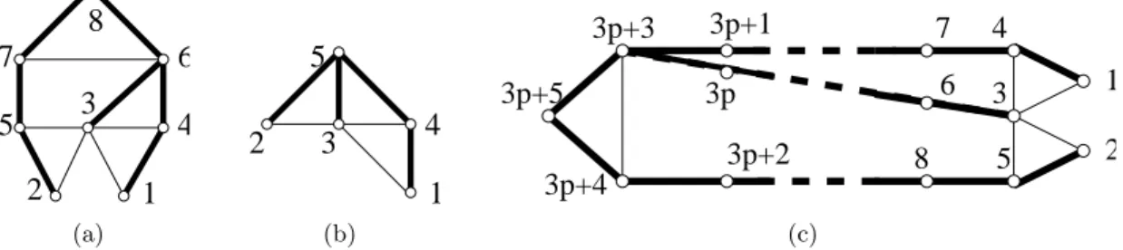
Figure 1: Lemmata 3 and 4 give optimal bounds.
(a) A 4-chordal graph G1 and a Strong-BFS-tree T1 such that Str(R(G1, T1)) = 3.
(b) A chordal graph G2 and a Max-BFS-tree T2 such that Str(R(G2, T2)) = 1.
(c) A 2p + 2-chordal graph G3 and a Max-BFS-tree T3 such that Str(R(G3, T3)) = 2p + 1.
the message along the path from x to y in T ; but, if at some step the message could go through an edge e ∈ E(G) \ E(T ) that leads to the branch of T containing y, then it will use such a shortcut. More formally, our routing scheme R(G, T ) is defined as follows.
If x = y, stop.
If there is w ∈ NG(x), an ancestor of y in T , choose such a vertex w minimizing dT(w, y);
Otherwise, choose the parent of x in T .
For instance, Figure 1 represents three graphs where spanning trees are depicted with bold edges. In Figure 1(a), a message from 1 to 2 will follow the path (1, 4, 6, 7, 5, 2). In Figure 1(b), the same message will follow (1, 4, 5, 2). Let us make some simple remarks.
1. The routing scheme R(G, T ) is well defined. Indeed, the message will eventually reach its destination since its distance to y in T is strictly decreasing at each step. Even if T were not a shortest paths tree, but an arbitrary rooted spanning tree of G, the message would eventually reach its destination. Indeed, in this case, the distance in T between the message and its destination y might not decrease in only one case that may occur at most once: at a step when the message stands at some descendant v of y such that v has a neighbor u (in G) which is an ancestor of y and dT(v, y) ≤ dT(u, y). In that case,
the message will be transmitted from v to u, possibly increasing the distance from the message to y in T . It is easy to check that it is the only case when this happens.
2. Once a spanning tree T rooted at an r ∈ V (G) has been defined, this scheme can be effi-ciently implemented. It is sufficient to label the vertices in a way where any rooted subtree of T corresponds to a single interval. Each vertex u stores the interval corresponding to the subtree of T rooted at v, for any neighbor v of u but its parent. Then, the routing function chooses the port corresponding to the inclusion-minimal interval containing the destination’s address, and it chooses the parent of the current location if no such interval exists. Note that this is not an interval routing scheme because some intervals may be contained in others.
3. Since we assume that T is a BFS-tree, it is easy to see that the route computed by the routing scheme R(G, T ) between two arbitrary nodes contains at most one edge that is not an edge of T . Indeed, after having taken such a shortcut, the message reaches y by following the path in T , which is a shortest path in G since T is a BFS-tree.
Theorem 3 Let k ≥ 3 and let G be a k-chordal graph.
• Let T be any Strong-BFS-tree of G. Then Str(R(G, T )) ≤ k − 1. • Let k = 3 and T be any Max-BFS-tree of G. Then Str(R(G, T )) ≤ 1. • Both bounds are tight.
3.2 Stretch in k-Chordal Graphs
Let k ≥ 3 and let G be a k-chordal graph and T be a (rooted) Strong-BFS-tree of G. Let x, y ∈ V be arbitrary source and destination, respectively. The proof is a case by case analysis to bound Str(R(G, T ), x, y). Let Rxy be the route from x to y computed by R(G, T ). In the
following, we compare the length of Rxy with the length of a shortest path between x and y in
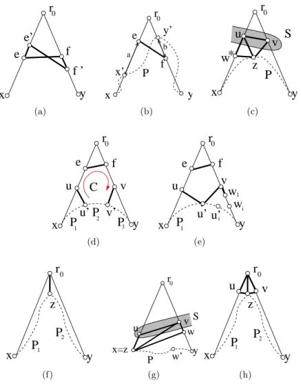
G. Several parts of the following discussion are depicted in Figure 2, where bold lines represent edges, thin lines represent paths belonging to T and dotted lines represent paths with edges not necessarily in T .
3.2.1 When the computed route and shortest path are not independent
In this subsection, we prove that it is sufficient to consider x and y with the least common ancestor r0 such that there is a shortest path P between x and y in G with no internal vertices
of P in V (Tx→r0) ∪ V (Tr0→y), i.e., P and the path with vertex-set V (Tx→r0) ∪ V (Tr0→y) are
independent.
If x is an ancestor or a descendant of y, Rxy is the path between x and y in T . Since T is a
BFS-tree, this is a shortest path. From now on, we assume that r0 ∈ V (G), the least common
ancestor of x and y, is distinct from x and y. By definition of R(G, T ), Rxyeither passes through
r0, or it uses an edge {e, f } ∈ E(G) \ E(T ) with e ∈ V (Tx→r0) \ {r0} and f ∈ V (Tr0→y) \ {r0}.
I.e., the route Rxy from x to y is either Tx→e∪ {e, f } ∪ Tf →y, or Tx→r0∪ Tr0→y.
First, we need a technical lemma that shows that the roles of x and y are somehow symmetric. Lemma 1 Str(R(G, T ), x, y) = Str(R(G, T ), y, x) and the route computed from x to y and the route computed from y to x are almost identical, i.e., they have the same length and differ in at most one vertex.
Proof. Let Rxy be the route computed by R(G, T ) from x to y. If Rxy passes through r0, then
there is no edge not in T between a vertex of Tx→r0 and a vertex of Tr0→y. In this case, Ryx
also passes through r0, and Rxy = Ryx. Similarly, if Ryx passes through r0, then Rxy = Ryx.
Now, let us assume that Rxy 6= Ryx. Hence, r0∈ R/ xy∪ Ryx and both paths contain exactly
one edge not in T . This case is illustrated in Figure 2(a). Let {e, f } and {e′, f′
} denote the edges in Rx,y\ T and Ry,x\ T , respectively. Note that there must be e′ ∈ V (Te→r0) \ {e} and
f′
∈ V (Ty→f) \ {f }. Because T is a BFS-tree, there is dG(r0, f ) < dG(r0, f′) ≤ dG(r0, e′) + 1 ≤
dG(r0, e) ≤ dG(r0, f ) + 1. Thus, e′ is the parent of e and f is the parent of f′. Therefore, if
Rxy 6= Ryx, Rxy = Tx→e∪ {e, f } ∪ {f, f′} ∪ Tf′→y, and Ryx= Ty→f′∪ {f′, e′} ∪ {e′, e} ∪ Te→x.
Now, let us have a look at the restrictions we can put on the shortest path that we will compare with the shortest path generated by the routing. Let P0be a shortest path in G between
x and y. Let y′ be the first vertex of P
0 in V (Tr0→y), and x
′ be the last vertex of P
0, before y′,
in V (Tx→r0). Let P
′ be the subpath of P
0 between x′ and y′. Notice that P′ has no internal
vertices in V (Tx→r0) ∪ V (Tr0→y). Because T is a Strong-BFS-tree, P0= Tx→x′∪ P
′∪ T
y′→y is a
shortest path between x and y in G. The following technical lemma restricts our investigation to the case where P0= P′, i.e., P0 has no internal vertices in V (Tx→r0) ∪ V (Tr0→y).
Lemma 2 Either Str(R(G, T ), x, y) = 0, or Str(R(G, T ), x, y) = Str(R(G, T ), x′, y′).
Proof. If x′ = y′ = r
0, then it is easy to see that P0 = Rxy. By definition, x′ and y′ must be
both equal to or different from r0. Therefore, let us assume both are different from r0. Recall
that Rxy = Tx→e∪{e, f }∪Tf →y, or Rxy = Tx→r0∪Tr0→y. In the second case, we set e = f = r0.
The proof is a case by case analysis according to the relative positions of x′ and e in T
x→r0, and
of y′ and f in T r0→y.
If Tx→e⊆ Tx→x′ and Tf →y ⊆ Ty′→y, then Str(R(G, T ), x, y) = 0 because |P′| ≥ 1.
Let us assume that Tx→x′ ⊂ Tx→eand Tf →y ⊂ Ty′→y. This case is illustrated in Figure 2(b).
Note that in this case e 6= f , therefore {e, f } ∈ E(G). Let a = |Tx→e| − |Tx→x′| > 0, and let b =
|Ty′→y| − |Tf →y| > 0. We study the layers of x, x′, y and y′to prove that Str(R(G, T ), x, y) = 0.
Let L = ℓ(e) be the layer of e. Then, ℓ(x′
) = L + a. Because {e, f } ∈ E(G) and T is a BFS-tree, L − 1 ≤ ℓ(f ) ≤ L + 1. Therefore, L − 1 − b ≤ ℓ(y′) ≤ L + 1 − b. However, because
T is a BFS-tree, we must have ℓ(x′
) ≤ ℓ(y′ ) + |P′ |. Thus, ℓ(x′ ) ≤ L + 1 − b + |P′ |. Finally, we get that a + b − 1 ≤ |P′ |. Since b > 0, then a ≤ |P′
|. To conclude, let us observe that |Rxy| = |Tx→x′|+a+1+|Ty′→y|−b = |P |−|P′|+a+1−b ≤ |P |. Hence, Str(R(G, T ), x, y) = 0.
If Ty→y′ ⊂ Tf →yand Te→x⊂ Tx′→x, the reasoning given above shows that Str(R(G, T ), y, x) =
0. By Lemma 1, we get that Str(R(G, T ), x, y) = 0.
Finally, if Tx→x′ ⊆ Tx→eand Ty′→y⊆ Tf →y, the route computed by R(G, T ) from x′ to y′ is
clearly Tx′→e∪ {e, f } ∪ Tf →y′. Moreover, Str(R(G, T ), x, y) = |Tx′→e∪ {e, f } ∪ Tf →y′| − |P′| =
Str(R(G, T ), x′, y′).
3.2.2 When the computed route and shortest path are independent
From Lemma 2, it remains to consider the case where there exists an xy-shortest path P in G with no internal vertices of P in V (Tr0→y) ∪ V (Tx→r0), where r0 is the least common ancestor
of x and y in T (cf. Figures 2(c)-2(f)). Basically, the proof proceeds by analyzing the distances in the cycle Tx→r0 ∪ Tr0→y∪ P and finding convenient chords in it.
Let S ⊆ V , NG(S) denotes the set of all vertices in V \ S with at least one neighbor in S.
Claim 1 If r0 ∈ N/ G(P ), there exist u in Tx→r0, u 6= x, and v in Ty→r0, v 6= y, such that
u, v ∈ NG(P ). Moreover, if G is chordal, u and v may be chosen adjacent: {u, v} ∈ E(G)\E(T ).
Proof. Since r0∈ N/ G(P ), the parents in T of x and y satisfy the first part of the claim. For the
second part, consider that G is chordal. Let Cr0 be the connected component of G \ NG(P ) that
contains r0. Let S = NG(Cr0) and let CP be the connected component of G \ S that contains
P . Notice that S ⊆ NG(P ) and it is an inclusion-minimal xr0-separator.
We can pick vertices u and v from the intersections of S with Tx→r0 and Tr0→y, respectively
(see Fig. 2(c)). Since S is a minimal separator in a chordal graph, S induces a clique [Gol04], Thus {u, v} ∈ E(G). Finally, {u, v} /∈ E(T ) because the opposite would imply that u or v is the a common ancestor of x and y, i.e., r0 ∈ {u, v}, a contradiction since u, v ∈ S. ⋄
Lemma 3 Let k ≥ 3. Let G be a k-chordal graph and let T be a Strong-BFS-tree of G. Then, for any x, y ∈ V (G), Str(R(G, T ), x, y) ≤ k − 1.
Proof. Recall that we only need to consider the following case: r0 is the least common ancestor
of x and y, and there exists a shortest xy-path P with no internal vertex in Tx→r0 ∪ Tr0→y. If
the route Rxy computed by R(G, T ) takes a shortcut, this edge is denoted {e, f }.
There are two cases to be considered. We first assume that r0 is not in the neighborhood of
f ’ r0 y x e f e’ (a) r0 e f x’ x y y’ a b P (b)
S
*
u
v
r
P
y
x
w
z
0 (c) C 0 f v P v’P y x u e u’ P r 2 1 3 (d) r0 f P y x u e u’ v w w u’ 1 1 i i (e)P
r
0z
y
x
P
1 2 (f) S P r y x=z u vw w’ 0 (g)z
v
y
x
P
P
r
0u
2 1 (h)Figure 2: Illustrations of different cases when bounding Str(R(G, T ), x, y). 2(a) Lemma 1, Rxy 6= Ryx. 2(b) Lemma 2, Tx→x′ ⊂ Tx→e and Tf →y ⊂ Ty′→y. 2(c) Claims 1, 8, 9 and 10.
2(f) Lemma 3, r0∈ NG(P ). 2(d) Lemma 3, r0∈ N/ G(P ), first item, case |P2| > 0. 2(e) Lemma 3,
r0 ∈ N/ G(P ), first item, case |P2| = 0. 2(g) Claim 5. 2(h) Lemma 4, r0∈ NG(P ).
Let us choose u and v as defined in Claim 1 and such that dG(u, r0) + dG(r0, v) is minimum.
We can assume that e ∈ Tr0→u and f ∈ Tv→r0 (possibly e = f = r0). Indeed, we can show the
following.
Claim 2 Let {e, f } be the ”shortcut” used in Rxy. If Tr0→e or Tr0→f has an internal vertex a
in NG(P ), then Str(R(G, T ), x, y) ≤ 2.
Proof. Indeed, suppose that the path Tr0→e has an internal vertex a in NG(P ). In other words,
there is a vertex a in the neighborhood of P , in the same branch as e and dG(x, a) > dG(x, e).
Let z denote a neighbor of a in P . Since T is a BFS-tree, dG(x, z)+1 ≥ dG(x, a), dG(r0, f )+1 ≥
dG(r0, e), and dG(r0, a) + 1 + dG(z, y) ≥ dG(r0, f ) + dG(f, y). So dG(x, z) ≥ dG(x, e), dG(r0, f ) ≥
dG(r0, a), dG(r0, f ) + 1 + dG(z, y) ≥ dG(r0, f ) + dG(f, y), and 1 + dG(z, y) ≥ dG(f, y). Finally,
dG(x, z) + 1 + dG(z, y) + 1 ≥ dG(x, e) + dG(f, y) + 1. Thus Str(R(G, T ), x, y) ≤ 2. By a similar
argument, b, an internal vertex of Tr0→f in NG(P ) results in Str(R(G, T ), x, y) ≤ 2. ⋄
f ∈ Tv→r0. In particular, this means that there are no edges between a vertex in Te→u and
Tv→f but {e, f }.
Let u′
∈ NG(u) ∩ P and v′ ∈ NG(v) ∩ P such that dG(u′, v′) is minimum. In the following
we assume that u′ is between x and v′ in P and let P = P
1∪ P2∪ P3, where P1 is the subpath
of P between x and u′, P
2 is the subpath of P between u′ and v′, and P3 is the subpath of P
between v′ and y. Otherwise, the proof is similar by setting P
1 to be the subpath of P between
x and v′, P
2 is the subpath of P between v′ and u′, and P3 is the subpath of P between u′ and
y.
By the choice of u, u′, v, v′
, the cycle C = {u, u′
} ∪ P2∪ {v′, v} ∪ Tv→f∪ {f, e} ∪ Te→u has no
chord. Thus, |C| = 3 + |P2| + |Tv→f| + |Te→u| ≤ k. Because T is a BFS-tree, |Tx→u| ≤ 1 + |P1|
and |Tv→y| ≤ 1 + |P3|. It follows that
|Rxy| = |Tx→u| + |Tv→y| + 1 + |Tv→f| + |Te→u| ≤ |P1| + |P3| + k − |P2|.
If |P2| > 0, |Rxy|−|P | = Str(R(G, T ), x, y) ≤ k −2|P2| < k −1 (cf., Figure 2(d)). Therefore,
let us consider the case when |P2| = 0, i.e., u′= v′ (cf., Figure 2(e)). We first consider the case
when u > v (in the BFS-ordering defining T ). There must be |Tv→y| ≤ |P3|. Indeed, suppose
|Tv→y| = |P3| + 1. This means that v is not the biggest vertex at distance dG(v, y) from y (u
is bigger) and, by Observation 1, y cannot be in the same branch as v in T - a contradiction. Hence,
|Rxy| = |Tx→u|+|Tv→y|+1+|Tv→f|+|Te→u| ≤ |P1|+|P3|−1+k−|P2| = k+|P1|+|P3|−1 = |P |+k−1.
Now, let us consider the case when u < v. Exchanging the roles of x and y, by symmetry, the above reasoning shows that Str(R(G, T ), y, x) ≤ k − 1. Now, applying Lemma 1, we again get that Str(R(G, T ), x, y) ≤ k − 1.
To conclude, let us assume that r0 ∈ NG(P ) (cf., Figure 2(f)). Let z ∈ NG(r0) ∩ P . Let
P = P1∪ P2 where P1 is the subpath of P between x and z, and P2is the subpath of P between
z and y. Because T is a Strong-BFS-tree, |Tx→r0| ≤ 1 + |P1| and |Tr0→y| ≤ 1 + |P2|. Therefore,
|Rxy| ≤ |Tx→r0| + |Tr0→y| ≤ |P1| + |P2| + 2 ≤ |P | + k − 1 (because k ≥ 3).
It is important to note that the previous result is valid for any Strong-BFS-tree. However, it is easy to observe that the inequality given by Lemma 3 is optimal. Indeed, Figure 1(c) represents a k-chordal graph with k = 2p + 2 (p ≥ 1) and a Strong-BFS-tree T (that actually is a Max-BFS-tree) such that Str(R(G, T ))) = 2p + 1 = k − 1: a message from 1 to 2 will pass through the edge {3p + 3, 3p + 4}.
Lemma 3 gives that, for any chordal graph G and a Strong-BFS-tree T , Str(R(G, T )) ≤ 2. The following lemma states that in the class of chordal graphs we can improve the stretch down to 1 by using a “better” BFS-tree, i.e., a Max-BFS-tree.
Lemma 4 Let G be a chordal graph and let T be a spanning tree defined by any Max-BFS-ordering. Then, for any x, y ∈ V (G), Str(R(G, T ), x, y) ≤ 1.
Proof. By Lemma 2, it is enough to consider the case when r0 is the least common ancestor of
x and y, P is a shortest path between x and y that is independent from Tx→r0∪ Tr0→y, i.e., the
only common vertices of P and Tx→r0∪Tr0→y are x and y. There are two cases to be considered.
1. We first assume that r0∈ N/ G(P ).
The proof consists of several simple claims. This case is illustrated in Figures 2(c) and Figure 2(g).
Let us choose u and v as defined in Claim 1. Note that {u, v} ∈ E because G is chordal. Therefore, by definition of the routing scheme, and because T is a shortest paths tree:
Claim 3 |Rxy| ≤ |Tx→u| + 1 + |Tv→y|.
Claim 4 u and v have a common neighbor z in P .
Proof. Let u′ and v′ be neighbors of u and v respectively in P . u′ and v′ are chosen in
order to minimize the length of the subpath P′of P between u′ and v′. Consider the cycle
{u, v} ∪ {v, v′
} ∪ P′
∪ {u′
, u}. Note that it is an induced cycle and, because G is chordal,
has to be a triangle. Thus u′ = v′ = z. ⋄
Let z be a common neighbour of u and v in P . Claim 5 If z ∈ {x, y}, Stretch(R(G, T ), xy) ≤ 1.
Proof. We assume z = x (the case z = y is symmetric). This case is illustrated in Figure 2(g). By construction, there is |Rxy| ≤ 1 + |Tv→y| and |Tv→y| ≤ 1 + |P |. If
|Tv→y| ≤ |P |, Str(R(G, T ), x, y) ≤ 1. So we only have to consider the case |Tv→y| = |P |+1.
Let w be the child of v in Tv→y. If {x, w} ∈ E, then |Rxy| ≤ 1 + |Tw→y| ≤ |P | + 1 and
Str(R(G, T ), x, y) ≤ 1. We prove that {x, w} ∈ E.
Because {u, v} ∈ E, ℓ(u) − 1 ≤ ℓ(v) ≤ ℓ(u) + 1. If ℓ(v) = ℓ(u) + 1, then ℓ(y) = ℓ(v) + |Tv→y| = ℓ(u) + 2 + |P |. Besides, ℓ(y) ≤ ℓ(x) + |P |. Since ℓ(x) = ℓ(u) + 1, we get a
contradiction. Now, let us assume ℓ(v) = ℓ(u) − 1. In this case, v > u and v should be the parent of x in a Strong-BFS-tree T , but we have {u, x} ∈ E(T ) and {v, x} ∈ E \ E(T ) - a contradiction. Finally, if ℓ(v) = ℓ(u), let w′
be a vertex in P \ {x, y}. If ℓ(w′
) ≤ ℓ(x), then ℓ(v)+|Tv→y| = ℓ(v)+1+|P | = ℓ(y) ≤ ℓ(w′)+|P |−1 ≤ ℓ(x)+|P |−1 = ℓ(u)+|P | = ℓ(v)+|P |
- again a contradiction. Therefore, ℓ(w′) > ℓ(x) for any w′
∈ P \ {x, y}. This implies that, for any w′ ∈ P \ {x, y}, ℓ(w′) − ℓ(v) > 1 and thus, {v, w′} /∈ E (property of levels
in a BF S tree). Also, for any vertex w′′
∈ Tv→y\ {w, v}, {v, w′′} /∈ E because Tv→y is a
shortest path. To conclude, let us consider the cycle P ∪ Ty→v∪ {v, x}. Since G is chordal,
we must have {x, w} ∈ E. ⋄
Therefore, let us assume that z /∈ {x, y}.
Moreover, let us assume that u > v (otherwise, we prove symmetrically that Str(R(G, T ), y, x) ≤ 1 and Lemma 1 allows to conclude).
Let P1 be the subpath of P between x and z, and let P2 be the subpath of P between z
and y. Because Tx→u and Tv→y are shortest paths, we get:
Claim 6 |Tx→u| ≤ |P1| + 1 and |Tv→y| ≤ |P2| + 1.
Claim 7 |Tv→y| ≤ |P2|.
Proof. Indeed, suppose |Tv→y| = |P2| + 1. This means that v is not the biggest vertex
at distance dG(v, y) from y (u is bigger) and, by Observation 1, y cannot be in the same
branch as v in T - a contradiction. ⋄
Let w∗ be the child of u in T
u→x. Next three claims are illustrated in Figure 2(c).
Proof. As above, z > w∗would contradict x being in the same branch as w∗. To conclude,
if {u, z} /∈ E(T ), then the parent of z in T must be strictly bigger than u, which implies that z > w∗, a contradiction.
⋄ Claim 9 If |Tx→u| = |P1| + 1, then {w∗, z} ∈ E.
Proof. Let us consider the cycle C = {u, w∗} ∪ T
w∗→x ∪ P1 ∪ {z, u}. For any vertex
t ∈ C \ {u, w∗
, z}, because |Tx→u| = |P1| + 1, ℓ(t) ≥ ℓ(u) + 2. Therefore {u, t} /∈ E. By
chordality of G and because |C| ≥ 4, {w∗
, z} ∈ E. ⋄
Claim 10 If |Tx→u| = |P1| + 1, then v > w∗.
Proof. Let v′ be the parent of v in T . We first prove that v′ > u. Since u > v and
{u, v} ∈ E \ E(T ), ℓ(u) ≤ ℓ(v) ≤ ℓ(u) + 1. If ℓ(u) = ℓ(v), then ℓ(u) = ℓ(v′) + 1 and v′ > u.
Otherwise, ℓ(u) = ℓ(v′), u and v′
are both adjacent to v and {v′
, v} ∈ E(T ). Hence, v′ > u. Since the parent of v is bigger than the parent of w∗, we obtain that v > w∗. ⋄
Claim 11 If |Tx→u| = |P1| + 1, then {w∗, v} ∈ E.
Proof. By Claims 8 and 10, we get v > w∗
> z. Moreover, by Claim 9, {w∗
, z} ∈ E. By definition of z, {z, v} ∈ E. By Theorem 2, the ordering defined by a Max-BFS is a PEO, therefore, {w∗
, v} ∈ E. ⋄
We are now ready to prove first case of Lemma 4. If the common neighbor z of u and v in P (z exists by Claim 4) is either x or y, then the result follows from Claim 5. Otherwise, by Claim 6, |Tx→u| ≤ |P1| + 1. By Claims 7 and 11, it follows that |Tv→y| ≤ |P2|
and, either |Tx→u| ≤ |P1|, or |Tx→u| = |P1| + 1 and {w∗, v} ∈ E. If |Tx→u| ≤ |P1|, by
Claim 3, Str(R(G, T ), x, y) ≤ 1. Otherwise, because {w∗
, v} ∈ E and by definition of the routing scheme, |Rxy| ≤ |Tx→w∗| + 1 + |Tv→y| and then |Rxy| ≤ |P1| + 1 + |P2|, i.e.,
Str(R(G, T ), x, y) ≤ 1. This proves the first case of Lemma 4. 2. Let us now assume that r0∈ NG(P ).
Let z ∈ NG(r0) ∩ P , let u be the child of r0 in Tr0→x and let v be the child of r0 in Tr0→y.
This case is illustrated in Figure 2(h).
First, let us consider the case z = x (or symmetricaly z = y). Because Tr0→y is a
shortest path, |Tr0→y| ≤ 1 + |P |. Moreover, |Rxy| ≤ 1 + |Tr0→y|. Hence, if |Tr0→y| ≤ |P |,
Str(R(G, T ), x, y) ≤ 1. Therefore, let us consider the case when |Tr0→y| = 1 + |P |. In
particular, y 6= v because |P | > 0. If {z, v} ∈ G, |Rxy| ≤ 1 + |Tv→y| ≤ 1 + |P |, and
Str(R(G, T ), x, y) ≤ 1. It remains to prove that {z, v} ∈ G. Let us consider the cycle C = {r0, v}∪Tv→y∪P ∪{z, r0}. For any vertex t ∈ C \{r0, z, v}, because |Tr0→x| = |P |+1,
ℓ(t) ≥ ℓ(r0)+2. Therefore {v, t} /∈ E. By chordality of G and because |C| ≥ 4, {z, v} ∈ E.
Therefore, let us assume z /∈ {x, y}. Let P1 be the subpath of P between x and z, and let
P2 be the subpath of P between z and y. Because Tx→r0 and Tr0→y are shortest paths:
Claim 12 |Tx→r0| ≤ |P1| + 1 and |Tr0→y| ≤ |P2| + 1.
Claim 13 If |Tx→r0| ≤ |P1| or |Tr0→y| ≤ |P2|, Str(R(G, T ), x, y) ≤ 1.
From now on, let us assume that |Tx→r0| = |P1| + 1 and |Tr0→y| = |P2| + 1. Similarly
to the above case when z = x, we prove that {z, v} ∈ E and {z, u} ∈ E. By mimicking the proof of Claim 8, we get that z < min{u, v}. By Theorem 2, the ordering defined by a Max-BFS is a PEO, therefore, {u, v} ∈ E. Then, |Rxy| ≤ |Tx→u| + 1 + |Tv→y|, and
Str(R(G, T ), x, y) ≤ 1. This concludes the proof of the second case of Lemma 4.
It is easy to observe that the inequality given by Lemma 4 is optimal. Indeed, consider Figure 1(b) and the route between 1 and 2. The above discussion and lemmata prove Theorem 3.
4
Distributed algorithm
In this section we present a simple distributed algorithm that computes the routing tables sufficient for the execution of the routing scheme described in the previous section. Recall that the time-complexity of the algorithm is defined by the number of communication steps. We neglect the time needed for computations performed locally, since passing messages between the nodes is considered several orders of magnitude slower. To reinforce this point of view let us point out that the local computations used by the algorithm are not complex. Actually, the most costly computation performed by the nodes during each step of the execution of our distributed algorithm consists in lexicographically ordering ∆ labels of at most D integers of log D bits which can be done in time ∆D.
Before describing the algorithms for computing routing schemes, let us give an informal description of the procedure. The computation of routing schemes consists of three phases. The first two of them aim at building a Strong/Max-BFS-tree T . For this purpose, the first phase chooses an arbitrary vertex as the root and gives to any vertex its layer, i.e., its distance to the root. The second phase is divided into rounds. During the ith round, each vertex in layer i decides its parent in layer i − 1 and the vertices in layer i − 1 order their children. The ordering process is done simultaneaously for all vertices in layer i − 1, in time O(1) in the case of a Strong-BFS-tree, resp., in time O(∆) in the case of a Max-BFS-tree. Then, during the third phase, each vertex x is assigned an integral label P (x) that corresponds to its position in a DFS postorder traversal of T . It is easy to check that it gives a Strong/Max-BFS-ordering of G. Moreover, x learns I(x), the interval corresponding to the labels of its descendants in T (including x). P (x) is used as the identifier of x in the routing scheme. At each vertex y, for every neighbor x of y (except for the parent of y), the edge yx is labeled with I(x).
Let us describe the algorithm in detail.
1st Phase. The first phase chooses an arbitrary vertex r ∈ V (G) as the root and gives to each vertex its layer, i.e., its distance from r. Moreover, each vertex informs its neighbors of its own layer. This trivially takes at most D + 1 steps by broadcasting a counter initially set to 1 by the root. Now, if each vertex chooses an arbitrary neighbor in the lower layer as the parent, the obtained graph is a BFS-tree. However, when Strong-BFS-trees or Max-BFS-tree are considered, a particular neighbor in the lower layer must be chosen as parent.
2nd Phase. The second phase aims at determining an appropriate parent for each vertex. For this purpose, we assign an ordering on the vertices based on the following labeling: the root receives an empty label and any vertex v ∈ V (G) in the layer i ≥ 1 will eventually have a full label label(v), where label(v) is a sequence of i integers that consists of the full label of its parent u concatenated with the integer p that indicates that v is the pth child of u. In the
following, a partial label is a prefix of a full label that will eventually be computed. Note that, if two nodes u and v have same partial label with size i ≥ 1, i.e, the first i integers of their full labels are equal, then u and v have the same ancestors in layers 0 to i. Roughly, the label of a vertex v defines a path from the root to v. The labels will be constructed gradually, in a way that each vertex will be aware of the current (partial) labels of its neighbors. Notice that the lexicographic ordering of full labels gives the inverse of the Strong-BFS-ordering (or Max-BFS-ordering) under construction. Transforming it into integer numbers ranging from n down to 1 can be easily computed once we have fixed T and ordered the children of each node (see the third phase).
The second phase is devided into D rounds. At the end of the ith round, vertices of layer
i ≥ 1 have learnt their full label, while the vertices of layer i + 1 know their partial label of length i. The vertices in layer i + 1 also know the full label of their neighbors in layer i and they can choose as parents the one among these neighbors with smallest full label. Then, during the (i + 1)th round, the vertices of layer i order their children so that any vertex v in layer
(i + 1) learns the last integer of its (full) label. This takes time O(1) when Strong-BFS-trees are considered, and time O(∆) when Max-BFS-trees are considered. Once, this integer has been computed, the vertex v propagates it toward layers > i + 1. This spreading of messages of size O(log n) bits is done simultaneously to next rounds, in such a way that when round j occurs, the vertices in layer j actually know their partial label of length j − 1.
Spreading of labels. Let us describe how to spread the labels of the vertices efficiently, that is, using messages of size O(log n) bits and in time O(D).
It is easy to check that the following process ensures that k ≥ 0 steps after the end of the ith round (i ≥ 1), the vertices in layer i + k + 1 have learnt their partial label of length i and
the partial label of length i of their neighbors in layers i + k + 1 and i + k. In particular, this ensures that before the beginning of roud i + 1, all vertices of layer i + 1 know the full label of their neighbors in layer i and their own partial label of length i.
For any i ≥ 1, each vertex v in the layer i maintains a subset P P (v) (for potential parent) of its neighbors in layer i − 1 that initially contains all these neighbors. Roughly, at any step of the algorithm, all vertices in P P (v) will have the same partial label which correponds to the partial label of v at this step. When all vertices in P P (v) receive a new integer to be added in their partial label, they forward it to v that only keeps as potential parents the vertices in P P (v) with smallest partial label.
More formally, once a vertex v in layer i has received its full label with last integer pv (that
corresponds to its position among its siblings), it transmits the pair (i, pv) to all its neighbors.
Then, its neighbors in layer i + 1 must propagate this information toward the layers j > i + 1. To avoid flooding, we proceed as follows, any vertex considering only the messages coming from its potential parents. When a vertex v in the layer j > i has received such a message (i, pu)
from all of its neighbors u in P P (v), this means that, at this step, the partial labels of the vertices in P P (v) have length i and differ only in their ith element. That is to say, there is a sequence of i − 1 integers L such that for any u ∈ P P (v), the label of u is L concatenated with pu. Moreover, L is the partial label of v at this step. Then, v keeps in P P (v) the vertices that
have the smallest partial label (in the lexicographic ordering): let p be smallest integer such that v has received (i, p) from its neighbors in P P (v), then v keeps in P P (v) all the vertices with new partial label L concatenated with p. Then, v adds p in its own partial label and transmits the corresponding pair (i, p) to all its neighbors. Moreover, receiving such a message from any neighbor u′, v adds p to the locally stored (partial) label of u′. Proceeding in this way, once all
vertices v in layer i have received a label, every vertex in layer i + 1 knows its potential parents, i.e., its neighbors in P P (v), and the corresponding label.
Ordering of children in Strong-BFS-tree. Once each vertex in layer i has chosen a parent, the vertices in layer i − 1 establish an ordering on their children. If we want to obtain a Strong-BFS-tree without additional properties, any ordering is valid. Therefore, each vertex in the layer i − 1 arbitrarily orders its children and sends them their position in this ordering. Then, each vertex in layer i has a full label. This takes one step per layer, i.e., time O(D) in total. Ordering of children in Max-BFS-tree. In this case, each vertex in layer i − 1 will order its children according to the number of neighbors with smaller labels they have. In other words, each vertex in layer i − 1 orders its children according to the number of their neighbors that will have larger numbers in the final ordering. Notice that as soon as the vertices of layer i have chosen their parent and broadcasted them to their neighbors, a vertex v in layer i only needs to learn its position in the ordering relatively to its siblings in T .
Note that, by definition of Max-BFS, the order of the children of a vertex in layer i − 1 does not depend on the order of the children of another vertex in layer i − 1. The children of vertices in layer i − 1 appear as consecutive blocks in layer i and it is only important to know which blocks appear earlier and which ones appear later in the ordering. Therefore, the children of each vertex u from layer i − 1 can be ordered in parallel, based on the number of their neighbors in layer i − 1, or in layer i and with a father placed before u in layer i − 1.
A vertex u in layer i − 1 orders its children as follows. Let us assume u has already ordered its first p children (p ≥ 0). These neighbors of u have full labels while remaining neighbors of u only have partial label. By definition of a Max-BFS-ordering, u chooses its p + 1st child v as the one with the biggest number of neighbors with bigger labels (than v), i.e., v is the child with the biggest number of neighbors that either have a parent bigger than u or that are siblings of v with a full label. v receives p + 1 from u and completes its label (that becomes full). Then, v informs its siblings that it has received a full label, and each child of u updates the number of its neighbors that already have full labels. In this way, u orders its d(u) children in O(d(u)) time. So, in total, this step is executed in O(∆) time per layer. Therefore, in at most O(min{∆D, n}) steps, every vertex has chosen a unique vertex as its parent and the tree T rooted in r is well defined.
3rd Phase. The third phase consists in assigning to each vertex v his position in the ordering and the interval of positions of vertices that belong to Tv, the subtree of T rooted in v. It is
easy to do so by two stages, the first one consisting in propagation of messages from the leaves toward the root and the second one from the root toward the leaves. During the first stage, the leaves of T send 1 to their parents, and every vertex u with children v1, · · · , vr receives from
vi (1 ≤ i ≤ r) the number ℓi of vertices belonging to the subtree of T rooted in vi and sends
to its parent 1 +Pi≤rℓi. During the second stage, the root is assigned the position n and the
interval [1, . . . , |V (G)|]; each vertex v takes the last position in the interval it has received and partitions the rest into subintervals corresponding to each of its children. It is easy to check that the resulting ordering corresponds to a DFS postorder traversal of T . This phase takes at most 2D steps. The discussion of this section can be summarized with the following theorem. Theorem 4 The distributed protocol described above computes routing tables of O(∆ log n) bits per node for any n-node network G with diameter D and maximum degree ∆. Moreover, our distributed protocol is executed in time O(D) if the tree T (implicit in the table) is an arbitrary Strong-BFS-tree, and in time O(min{∆D, n}) if T is a Max-BFS-tree. The routing tables produced by our prococol are the one used by the routing scheme described in Section 3.
The distributed protocol described in this section has been implemented on a simulator and has been tested for various topologies [HPT09]. For each topology, and for each networks’ size in {500, 1000, · · · , 3500}, 100 random instances of networks with the considered topology have
been tested. The results obtained via the simulations correspond to theoretical results. In particular, an empiric argument for the correctness of the implementation is that, in chordal graphs, the additive stretch never exceeds 1. Non surprisingly, in grid topologies which include many big holes, our protocol achieves poor performances (roughly, an average additive stretch of n is obtained for the n × n grids). Further, the protocol behaves very well on power law networks (generated using the preferential attachment method) which are considered to be good representations of real world complex networks [BA99]. Indeed, in this kind of networks, our protocol achieves an average (resp., maximum) additive stretch less than 1 (resp., 5).
5
Open Problems
Many questions remain open in this study. In particular: Is it possible to design a routing scheme achieving the same stretch and time-complexity but using smaller routing tables? What can we say about the stretch if few large cycles are allowed? Routing schemes in dynamic networks, i.e., when nodes are free to leave or to arrive in the network at any time, are needed. Fault-tolerant and self stabilizing algorithms to compute routing tables would be of much interest.
The authors would like to thank Feodor F. Dragan for valuable discussions during his stay at CMM, Universidad de Chile.
References
[AG06] I. Abraham and C. Gavoille. Object location using path separators. In Proceedings of the 25th Annual ACM Symposium on Principles of Distributed Computing (PODC), pages 188–197, 2006. [AGGM06] I. Abraham, C. Gavoille, A.V. Goldberg, and D. Malkhi. Routing in networks with low doubling
dimension. In Proceedings of the 26th IEEE International Conference on Distributed Computing Systems (ICDCS), page 75, 2006.
[AP90] B. Awerbuch and D. Peleg. Network synchronization with polylogarithmic overhead. In Proceedings of the 31st IEEE Symposium on Foundations of Computer Science (FOCS), pages 514–522, 1990. [BA99] A.-L. Barabasi and R. Albert. Emergence of scaling in random networks. Science, 286:509–512, 1999. [BKS05] A. Berry, R. Krueger, and G. Simonet. Ultimate generalizations of lexbfs and lex m. In Proceedings of the 31st International Workshop on Graph-Theoretic Concepts in Computer Science (WG), pages 199–213, 2005.
[CK08] Derek G. Corneil and Richard M. Krueger. A unified view of graph searching. SIAM Journal on Discrete Mathematics, 22(4):1259–1276, 2008.
[DG02] Y. Dourisboure and C. Gavoille. Improved compact routing scheme for chordal graphs. In Proceedings of the 16th International Conference on Distributed Computing (DISC), pages 252–264, 2002. [Dou05] Y. Dourisboure. Compact routing schemes for generalised chordal graphs. Journal of Graph
Algo-rithms and Applications, 9(2):277–297, 2005.
[Dra05] F. F. Dragan. Estimating all pairs shortest paths in restricted graph families: a unified approach. Journal of Algorithms, 57(1):1–21, 2005.
[FG65] D. R. Fulkerson and O. A. Gross. Incidence matrices and interval graphs. Pacific Journal Mathe-matics, 15:835–855, 1965.
[FG01] P. Fraigniaud and C. Gavoille. Routing in trees. In Proceedings of the 28th International Colloquium on Automata, Languages and Programming (ICALP), pages 757–772, 2001.
[Fra05] P. Fraigniaud. Greedy routing in tree-decomposed graphs. In Proceedings of the 13th Annual European Symposium on Algorithms (ESA), pages 791–802, 2005.
[Gav00] C. Gavoille. A survey on interval routing. Theoretical Computer Science, 245(2):217–253, 2000. [GG01] C. Gavoille and M. Gengler. Space-efficiency for routing schemes of stretch factor three. Journal of
Parallel and Distributed Computing, 61(5):679–687, 2001.
[GP96] C. Gavoille and S. Perennes. Memory requirements for routing in distributed networks (extended abstract). In Proceedings of the 15th Annual ACM Symposium on Principles of Distributed Computing (PODC), pages 125–133, 1996.
[GP99] C. Gavoille and D. Peleg. The compactness of interval routing. SIAM Journal on Discrete Mathe-matics, 12(4):459–473, 1999.
[GP01] C. Gavoille and D. Peleg. The compactness of interval routing for almost all graphs. SIAM Journal on Computing, 31(3):706–721, 2001.
[HPT09] L. Hogie, D. Papadimitriou, and I. Tahiri. Alusim: simulating routing schemes on large-scale topolo-gies. Technical report, INRIA, aug 2009.
[NN98] L. Narayanan and N. Nishimura. Interval routing on k-trees. Journal of Algorithms, 26(2):325–369, 1998.
[PU89] D. Peleg and E. Upfal. A trade-off between space and efficiency for routing tables. Journal of the ACM, 36(3):510–530, 1989.
[SK85] N. Santoro and R. Khatib. Labelling and implicit routing in networks. The Computer Journal, 28(1):5–8, 1985.
[Tho04] M. Thorup. Compact oracles for reachability and approximate distances in planar digraphs. Journal of the ACM, 51(6):993–1024, 2004.
[TZ01] M. Thorup and U. Zwick. Compact routing schemes. In Proceedings of the 13th Annual ACM Symposium on Parallel Algorithms and Architectures (SPAA), pages 1–10, 2001.