Analysis of wave propagation in unbounded media

Publisher’s version / Version de l'éditeur:

Computers and Structures, 33, 4, pp. 1037-1045, 1989

READ THESE TERMS AND CONDITIONS CAREFULLY BEFORE USING THIS WEBSITE. https://nrc-publications.canada.ca/eng/copyright

Vous avez des questions? Nous pouvons vous aider. Pour communiquer directement avec un auteur, consultez la

première page de la revue dans laquelle son article a été publié afin de trouver ses coordonnées. Si vous n’arrivez pas à les repérer, communiquez avec nous à PublicationsArchive-ArchivesPublications@nrc-cnrc.gc.ca.

Questions? Contact the NRC Publications Archive team at

PublicationsArchive-ArchivesPublications@nrc-cnrc.gc.ca. If you wish to email the authors directly, please see the first page of the publication for their contact information.

NRC Publications Archive

Archives des publications du CNRC

This publication could be one of several versions: author’s original, accepted manuscript or the publisher’s version. / La version de cette publication peut être l’une des suivantes : la version prépublication de l’auteur, la version acceptée du manuscrit ou la version de l’éditeur.

Access and use of this website and the material on it are subject to the Terms and Conditions set forth at

Analysis of wave propagation in unbounded media

Hunaidi, O.

https://publications-cnrc.canada.ca/fra/droits

L’accès à ce site Web et l’utilisation de son contenu sont assujettis aux conditions présentées dans le site LISEZ CES CONDITIONS ATTENTIVEMENT AVANT D’UTILISER CE SITE WEB.

NRC Publications Record / Notice d'Archives des publications de CNRC:

https://nrc-publications.canada.ca/eng/view/object/?id=047e6d1c-c888-454d-9a42-caf43c8aa621 https://publications-cnrc.canada.ca/fra/voir/objet/?id=047e6d1c-c888-454d-9a42-caf43c8aa621

R e f

Ser

. .

TH

Natlonal Research Consail national

1

NEld

Council Canada de recherches Canada

1

no.

1640

1

IRC

( 3

I Institute for lnstitut de

Research in recherche en

I

I Construction construction

Analysis of Wave Propagation in

Unbounded Media

by M. Osarna Al-Hunaidi

Reprinted from

Computers & Structures Val. 33. .

-

. .

-

-,

No.

. . . . 4.1989 , . . .

p. 1037-1045

(IRC Paper No. 1640)

NRCC 31115

Rtsumt

Une nouvelle approche est proposte pour knir cornpte de l'aspect ccinfiiitf5,

des milieux non b t s

analys6s au moyen de la m6thode des tl6ments finis

dans le domaine temps.

Le

milieu est divist en une dgion finie, qui

pdsente un int6dt dans l'analyse, et un milieu dsiduel non born6. L'apport

en rigidit6 de ce demier est bien repdsentt par la matrice d'influence de sa

limite avec la dgion finie; la matrice est calcul6e directement dans le

domaine temporel. Cette approche convient aux situations oh il faut

effectuer de nornbreuses analyses de la dgion finie.

Campurrs B Strucrvrns V o l 33, No. 4, pp. 1037-1045. 1989 W45.1949189 S3.W

+

0.00

Printed in Orrat Britain. Psigumon Prcar plc

ANALYSIS OF WAVE PROPAGATION I

UNBOUNDED, MEDIA

M. OSAMA AL-HUNAIDI

Structures Section, Institute for Research in Construction, National Rese Ottawa, Ontario, Canada KIA OR6

(Received 4 October 1988)

.

Abstract-A new procedure is presented to account for the radiation condition of

analysed using the finite-element method in the time domain. The medium is divided into a finite region that is of interest in the analysis, and the remaining unbounded medium. The stiffness contribution of the latter is properly represented by its boundary influence matrix, which is directly calculated in the time domain. This procedure is suited for situations in which many analyses of the finite region must be

performed.

I , .

4

1 1. INTRODUCrlON generally lower than the frequency range of interest,

In many problems of earthquake engineering and dynamic analysis of soil-structure interaction, nu- merical modelling of wave propagation is necessary. Numerical models involve discretization of the con- tinuum and if nonlinearities exist they also involve temporal discretization, i.e. the use of step-by-step time integration. The finite element method is one of the most popular discretization techniques because of its effectiveness in handling irregularities and compli- cated geometries. This method, however, divides the space domain into discrete elements, and can there- fore only deal with finite domains with well-defined boundaries. As such boundaries do not exist natu-

The third approach has been shown to be inappropri- ate [I]. These difficulties have motivated the develop- ment of so-called 'transmitting' or 'silent' boundaries. The function of these boundaries is to introduce appropriate force and/or displacement conditions to sim~alate the ..-- effect ---. of -. the .... .... truncated exterior infinite ~ ~~~ ~ ~

domain and hence preserve the real physical he- haviour of the problem. Many such boundaries have been developed and implemented for analyses in the time domain, with varying degrees of success. They represent only an approximation to the actual boundary condition [Z]. In general, they suffer from one or more of the following drawbacks:

rally, waves propagatmg towards these boundaries

will he reflected back into the model. his results in ~ ~ ~ ~~~~ ~~~~ ~~ .~~~ (1) they are effective only for a small range

false physical behaviour of the problem. To overcome incidence

this difficulty, analysts may consider the following (2) are to

approaches:

-

and

(3) they may fail under static loads. (I) use of a very large finite model so that waves

reflected at the model's artificial boundaries do not Consequently, use of a large model remains the arrive at the area of interest within the time period only available approach to solve wave propagation

over which the analysis is performed; problems directly with a high degree of accuracy in

(2) use of large finite elements to model as large a the time domain. This paper introduces an approach medium as possible with a minimum number of for the economical analysis of large models when

degrees of freedom; or many analyses of the same model are required. The

(3) introduction of material damping in the finite approach is designed for explicit time integration model to dissipate reflected wave energy before it methods. It is based on calculating a boundary

arrives at an area of interest. influence matrix by analysing an extensive model of

the exterior infinite domain in the time domain using The first approach may not be economical because unit triangular force pulses. This matrix is then used of its high storage and computational requirements. during the analysis of the interior finite model to The second approach is normally not accepted from calculate the boundary's response one time step an accuracy point of view. This is because finite ahead. The approach is exact and does not introduce elements act like 'low-pass' filters with a certain any approximations. Although the cost of calculating cut-off frequency that depends on the size of the the boundary influence matrix may be substantial, element-the larger the element, the lower its cut-off computational savings can be made for situations frequency. The cut-off frequency of large elements in which many analyses of the same problem are necessary to produce large economical models is required.

1038 M OSAMA AL-HUNAIOI

2. TIME DOMAIN BOUNDARY INFLUENCE element mesh wrth its surrounding nodes. Conse-

MATRIX (TDBIM) _{quently, the true behaviour of the problem is not}

For a linear finite element model, the equatlon of correctly calculated unless one prescribes the tlme motion has the general form history of boundary motion (or alternatively boundary reaction forces) which would take place in [Ml{ul +[Kl{u) =

{f

} (1) an extended model (1.e. a very large model in which no reflections occur). In other words, one always where [MI is the mass matrix, [K] 1s the stiffness needs to know the true response of the boundary matrix; and {

f

), {u), { i i ) are vectors of nodal forces, nodes one time step ahead of the last time station and displacements and acceleration, respectively For sim- prescribe it as a boundary condit~on to simulate the plicity, dampmg is not included. Equation (1) can be stiffness contribution of the exterior infinite domain.

solved by either explicit or tmpliat time integration Because the boundary's response is a function of the methods, but the proposed artificial boundary treat- wave incidence angle, wave frequency, wave type, ment is designed for explicit methods. Examples of etc., the only way to have the true response (i.e. with methods commonly used in wave propagation studies no reflections) in time domain analyses IS to use an

are the well-known explicit central difference method extended finite element mesh. The computational cost and the impliclt Newmark famlly of methods [3], of this analysis may become substantial if the prob- which includes the central difference method as a lem has to be analysed many times. In the solution special case

(b

= 0, y = 0.5). procedure expliuned next, an extended model s em- The stiffness matrix [K] and possibly the mass ployed only as a prehminary step to calculate a matrix [MI in eqn (1) couple every nod nite boundary influence matr~x

Wave propagation in unbounded med~a

0

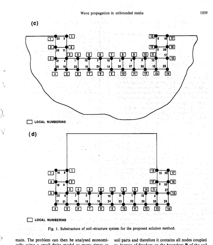
LOCAL NUMBERING

LOCAL NUMBERING

fig. I. Substructure of soil-structure system for the proposed solution method.

I

main. The problem can then be analysed economi- soil parts and therefore it contains all nodes coupled cally using a small fin~te model as many times as to degrees of freedom on the boundary B of the so11

I1

" J desired part The finite element equahons of the soil part and In the following procedure, the extended finite interface zone combined may be written in the follow-

'

element model, for example the soil-structure model ing form: shown in Fig. ](a), is substructured into three parts:

(1) structure, (2) soil, and (3) ~nterface zone, as shown 0

~n Fig. l(b). The structure part conslsts of the struc-

ture itself and a porhon of the supporting soil which mr;mbb

j{i!}

may be nonlinear and/or geometrically irregular. The

soil part must be linearly elastic (or linearly viscoelas- _kr

tic) and it should be sufficiently large for no

₊

[:

_{kfi ksfkbb}

kq{g=E](2)

refiect~ons at its far boundary to reach the boundary _{k, k, u,}

with the structure while the solutign a in progress.

The interface zone consists of one strip of elements In the above equation, the m and k matrices are (note. for the sake of simplicity, elements are assumed submatr~ces of the mass and st~ffness matrices of the here to be four-noded) that separate the structure and soil and interface zone substructures. The mass ma-

FORCE FORCE

t

t

1k

0 TIME

Rg 2 Untt triangular load pulse. trices are assumed to be diagonal. ti _{and u a}

acce1eratlon and d~splacement vectors, respectively

.f;

in eqn (2) andf; ~n Rg. I(b) are the attendmg internal nodal force vectors actlng on boundary I between the structure and interface zone. These forces are of equal magnitude but opposite directions.

S~milarly, the equations of motion for the finite nonlinear model, consisting of the structure part and interface zone Fig. l(d), are

The structure part can be nonlinear, but for sim- plicity it is considered linear in the above equation. In eqn (3), it is assumed that the response of boundary B, {u,), is known in advance and therefore it is a prescribed boundary condition and therefore the contribution k,&

.

u, is transferred to the right- hand side of the equilibrium equations.

Before solution of eqns (3), a time domain bounary influence matrix [Dl is calculated. This matrix de- scribes the response of boundary B degrees of free- dom resulting from unit triangular pulse forces (see Fig. 2) at degrees of freedom of boundary I. For instance, an element (i, j, k) of this matrix is defined as the response of degree of freedom i of boundary B a t time step k resulting from a unit triangular pulse force at degree of freedom j of boundary I. Matrix

[Dl is calculated by solving eqns (2) for unit triangu- lar pulse forces applied at degrees of freedom of boundary I, one at a time. The resulting response at degrees of freedom of boundary B is collected in matrix [Dl. This matrix is then used to calculate the displacements {u,) in eqns (3) as explained next.

As waves propagate from the structure part into the soil part, the attending internal nodal forces

{f;}

in Fig. I(d) can be considered to be the source of wave motion of degrees of freedom of boundary

B,

{u,}. For the purpose of calculating the boundary response {u,), the actual attending nodal forces

{A}

are broken down into triangular pulses as demon- strated in Fig. 3. If an explicit time integration soheme is used (at least for the interface zone), a non-zero

Rg 3 Representatton of force time history by triangular force pulses

say over time steps m and (m

+

I), will start only at the end of tlme step (m

+

1) or later [note for the central difference hme integration scheme it will start at the end of time step (m

+

211 Hence reflections from the boundary nodes to the interior nodes will commence after the end of time step (m

+

I). Conse- quently, the boundary's response may be calculated one time step ahead of the last time station using the attending nodal force vector

{f;)

at the last and past time stations and the boundary influence matrix [Dl

The previously d e t e m e d tlme doma~n boundary influence matrix is used to calculate the houndary's responses resulting from the triangular pulse compo- nents of the load by simple multiplication. The responses are then superimposed to obtain the boundary's displacement {u,) for the next time step.

3. NUMERICAL IMPLEMENTATION

displacement response at any of the degrees of free- Numerical implementation of the above solution dom on boundary B resulting from a triangular pulse, procedure using the time domain boundary influence

I

Wave propagat~on in unbounded rned~a 1041

matrix (TDBIM) may at first seem cumbersome. In equation are the same as for eqn (2). These forces are reality, its incorporation into existing finite element then stored in an array, called here F, as follows: wdes does not represent additional complications. In F(LFNEQ, ISTEP) = attending nodal force acting the following, a method is used that effectively gener- on degree of freedom number LFNEQ (local num- ates the boundary influence matrix ID1 using the soil ber) at the end of time step ISTEP.

substructure in Fig. I(c). The method also <ffectively calculates the attending nodal vector {A} and then calculates the boundary displacement vector { u b }

which is necessary for the analysis of the structure

, part in Fig. l(d). 3.1. Numbering technique

The finite element nodes in Fig. I(c) and (d) of the soil part and the structure, respectively, will usually have global node numbering that does not produce identical node numbers for nodes on the boundary Bin both models. The same is also true for nodes on the boundary I. For nodal points on these

, boundaries, a local node numbering is defined which coincides in numbers of both models as shown in Fig. l(c) and (d). The proposed treatment uses two arrays NATB and NCTB. Array NATB has as many element's as the maximum number of nodes on boundary B, say NNATB. It stores the global node number corresponding to each node on this boundary. Array NCTB has the same function as arrav

NATB

but for nodes on boundary I. Its dimension is NNCTB, which is the maximum~numher of nodes on boundary I. This information is then used to identify these nodes during the calculation of the boundary influence matrix and to extract the appropriate influence coefficients during the calcula- tion of the boundary response.

The boundary influence matrix [Dl is calculated using the extended soil model (see Fig. Ic), by applying unit triangular pulses to each degree of freedom of boundary I, one at a time. The resulting displacement time histories of degrees of freedom of boundary B are appropriately assembled into the matrix [Dl as follows: D (LBNEQ, LFENQ, IS- TEP) = displacement response at degree of freedom number LBNEQ of boundary B at time step ISTEP

-, resulting from unit triangular pulse force at degree of

freedom LFNEQ of boundary I, whereas all other DOE'S on I have zero forces (note: LBNEQ and

"

LFNEQ are local numbers for degrees of freedom on

7

boundaries B and I, respectively). 3.2. Calculation of internal forces

"

The calculation of the boundary's displacement using the time domain boundary influence matrix [Dl requires the availability of past time history of the attending nodal forces (1;) at boundary I. To calcu- late this force vector at the end of a time step, the equations of motion of the degrees of freedom for the boundary I are used as follows:

where the definitions of vectors and matrices in t h ~ s

3.3. Calculation of boundary displacement response

{ub}

To calculate the boundary displacement response one time step ahead of the last time station ISTEP, the amplitudes of triangular pulses composing the attending nodal force time history

{ A }

are multiplied by the corresponding influence coefficients of the boundary influence matrix [Dl and the results are then superimposed. For instance, the response of degree of freedom LBNEQ at the end of time step (ISTEP

+

1) is given by

LFNEQ STEP ~ B N , Q =

C C

W , k )

!-I k = I

D(LBNEQ, i, ISTEP

-

k

+

2). _{( 5 )} These boundary displacements are then prescribed

as boundary conditions at the truncation boundary of the finite model in Rg. I(d).

4. NUMERICAL EXAMPLE

To verify the proposed TDBIM procedure, a plane strain elasticity problem is considered. The problem is that of a layer which is underlain by a rigid base and subjected to a vertical line load at the surface. The finite element model and the corresponding boundary conditions used for this test problem are shown in Fig. 4. The finite element mesh consists of the structure part, interface elements and the soil part as mentioned previously. In this simple example, the structure part comprises only a small soil region which, for simplicity, is considered to be linearly elastic although in general the structure could be nonlinear, as discussed in Section 2. Bilinear isopara- metric elements are employed and they are all of the same size. The soil part of the finite element model is sufficiently large for the response of the boundary B

to be obtained for the duration of the test before any reflected waves arrive from the right boundary.

Material properties of the layer are summarized in Table 1. The surface vertical line load consists of a one-cycle sine pulse. The duration of the cycle is 15 sec and its amplitude is one unit. Time integration is performed with an implicit-explicit algorithm [3]. All elements are considered explicit and the integra- tion parameters employed are y = 0.5,

fl

*

0.0, time step At = 0.9 sec. The duration of the analysis is 120 time steps, which is equal to about seven load cycles. No damping is applied. Calculations are performed using double precision on an IBM 3090 computer. The vertical displacement response time history is recorded at point A of Fig. 4.

M:OSAMA AL-HUNAI

, ,

The finite element model in Fig.4(b), consisting of boundary response of the model in Fig. qc). Results the soil part and interface elements, is used to calcu- of the analysis which used the small model in Fig. q c ) late the time domain boundary influence matrix. This with the. TDBIM approach are then compared with matrix is stored and then recalled to calculate the the results of the extended mesh in Fig. 4(a), which

Wave propagat~on in unbounded media Table 1 . Material properties of layer system

S-wave velocity 0.5345 units/sec

P-wave velocity l unit/sec

Poisson's ratio 0.3

Unit density 1.0

are called the reference. solution. As expected, the resulting time history at point A for the

TDBIM

solution coincides with the reference solution. The difference cannot be resolved within the scale of the drawings and it has t o be marked by circles as shown in Fig. 5. The time domain boundary influence matrix

(b)

calculated for this problem may be stored for future use with the same problem, for different loading

conditions and/or different material properties of the STANDARD

structure part. VISCOUS

As an extension to this test problem, the efficiency BOUNDARY

\I

1.

. of the popular standard viscous silent boundary [4] is

,,'

examined. The purpose of this test is to demonstrate Fis 6. Finite element models using standard viscous

the approximation involved when using such local boundary: (a) small model; (b) large model.

5,: silent boundaries. Two locations of the lateral silent

boundary are tested. The first,is at a lateral distance surface points A, B and C. The response obtained by equal to one layer depth and the second is at a lateral using this viscous boundary is compared with the distance equal to twice the layer's depth, as shown in reference solution which was calculated previously Fig. 6. Vertical displacement response is recorded at using an extended mesh.

-

-

REFERENCE SOLUTION,

- - -

STO. VISCOUS ED.

0 20 40 60 80 100 120

TIME-SECOND

-

? REFERENCE SOLUTION,

- - -

STO. VISCOUS 60.

N 9 b

-

5

C

Y %

5

e

2

-

0

1

9 Y Fig, 7. Vertical displa

I _i Y! h I I I 0 20 40 60 80 I00 120

TIME-SECOND

-

REFERENCE SOLUTION,

- - -

STO. VISCOUS ED.

Fig. 8.

0 20 40 60 80 100 120

TIME-SECOND

0 20 40 60 80 100 120

TIME-SECOND

Vertlcal d~splacement response: comparison between reference solutlon and large model employing

vlscous boundary (a) at point A, (b) at polnt B, (c) at polnt (C)

Results of the small model, shown in Fig 7, are not in good agreement w ~ t h the reference solution. Re- sults of the larger model, shown in Rg. 8, represent substantial improvement over the results of the small model for polnts A and B but the response at point C located beside the boundary is poor. This means that for the viscous boundary, more accurate answers at polnt C require that the boundary be moved further away.

5. SUMMARY

An economical and accurate method IS presented

for the analysis of problems involving wave propaga- tion m unbounded media. The method uses an Influence matrix, calculated in the time domain, for the boundary between the finlte model of Interest and the truncated unbounded domain. During analysis of the finite model, this matrix is used to calculate the

Wave propagallon in unbounded media 1045

boundary's response one tlme step ahead. This re- Th~s paper is a contnbution of the Instttute for Research In

sponse is then used to simulate the stiffness contribu- Construction, Nat~onal Research Council of Canada tlon of the truncated unbounded domain and hence

preserve the real phys~cal behaviour of the problem.

The advantage of this procedure is that the boundary matrix can he used for as many analyses as desired of

the fin~te model at minimal additional computational

cost. The load conditions, geometry and material properties of the finite model are arhitraty.

In the numerical sense, the formulation of this method and the results obtained are exact.

REFERENCES

J. E. Luco, A. H. Hadjian and H. D. Bos, The dynamic

modeling of the half-plane by finite elements. Nucl. Engng Des. 31, 184-194 (1974).

E. Kausel, Local transmitting boundaries. J, Engng

Mech. 114, 1011-1027 (1988).

T. J. R. Hughes and W. K. Liu, implicit-explicit finite

elements in transient analysis: implementation and nu- merical examoles. J . aool. Mech. 45. 375-378 (1978). ~~~~~~~~~~ ~~~

4. J. ~ ~ s r n e r and R. L. ~ h i l e m e ~ e r , ~ i n i t e dynamic model

Acknowledgements-The author wishes to express his ap- for infinite media. J. Engng Mech. Div., ASCE 95,