Coupling between Monte Carlo neutron transport and thermal-hydraulics for the simulation of transients due to reactivity insertions

HAL Id: tel-02406396

https://tel.archives-ouvertes.fr/tel-02406396

HAL is a multi-disciplinary open access

archive for the deposit and dissemination of sci-entific research documents, whether they are pub-lished or not. The documents may come from teaching and research institutions in France or abroad, or from public or private research centers.

L’archive ouverte pluridisciplinaire HAL, est destinée au dépôt et à la diffusion de documents scientifiques de niveau recherche, publiés ou non, émanant des établissements d’enseignement et de recherche français ou étrangers, des laboratoires publics ou privés.

to reactivity insertions

Margaux Faucher

To cite this version:

Margaux Faucher. Coupling between Monte Carlo neutron transport and thermal-hydraulics for the simulation of transients due to reactivity insertions. Physics [physics]. Université Paris Saclay (CO-mUE), 2019. English. �NNT : 2019SACLS387�. �tel-02406396�

Th

`ese

de

doctor

at

NNT

:2019SA

CLS387

transport and thermal-hydraulics for the

simulation of transients due to reactivity

insertions

Th`ese de doctorat de l’Universit´e Paris-Saclay pr´epar´ee `a l’Universit´e Paris-Sud Ecole doctorale n◦_{576 Particules, Hadrons, ´Energie, Noyau, Instrumentation, Image,}

Cosmos et Simulation (PHENIICS)

Sp´ecialit´e de doctorat : ´Energie nucl´eaire

Th`ese pr´esent´ee et soutenue `a Saclay, le 18 octobre 2019, par

M

F

Composition du Jury : Sandra Dulla

Professeur, Politecnico di Torino (Italie) Rapporteur Elsa Merle

Professeur (HDR), CNRS/LPSC Rapporteur

Cheikh M’Back´e Diop

Directeur de recherche, CEA/DEN Pr´esident

Jan Dufek

Professeur, KTH Royal Institute of Technology (Su`ede) Examinateur Adrien Gruel

Ing´enieur-chercheur, CEA/DEN Examinateur

Emmanuel Gobet

Professeur (HDR), ´Ecole Polytechnique Directeur de th`ese Andrea Zoia

Ing´enieur-chercheur (HDR), CEA/DEN Directeur de th`ese Davide Mancusi

I am writing these lines while this Ph.D. is ending. This is the moment when I am thinking about all the people who were part of this adventure. Whether for scientific help or for friend support, I am thinking about a lot of people.

I would like to start by thanking Elsa Merle and Sandra Dulla for reviewing my thesis. I am deeply grateful for their careful reading and their comments on it. I am also grateful to Adrien Gruel and Jan Dufek for being part of the examining committee, and to Cheikh Diop for assum-ing the presidence of the jury.

It was an honour for me to do this thesis under the direction of Andrea Zoia. Thank you for giving me this opportunity and for all the interesting discussions we had and the ideas we shared. I would like to express my gratitude to Emmanuel Gobet for accepting the co-direction of my thesis. I have learnt a lot during our work sessions at ´Ecole Polytechnique and I re-ally want to thank you for the time you took when I had very little knowledge in the field of stochastic differential equations. To my supervisor Davide Mancusi, you asked me what I regret about this thesis, I can tell you that doing it under your supervision is the first thing I do not re-gret. Thank you for letting your door always open and to share your infinite knowledge with me.

I really enjoyed being involved in the McSAFE project, and doing joint works with KIT and VTT teams. I would like to thank them for that, with a special thank to Diego Ferraro and Manuel Garcia from KIT. Thank you for your kindness and all the discussions we had for the simulations of TMI and Spert. This joint work has taught me a lot. I wish you the best in your future dynamic works!

Je souhaite remercier ma famille qui m’a toujours beaucoup soutenue, en commenc¸ant par ma m`ere. Merci de m’avoir toujours encourag´ee. Venir faire cette th`ese `a Paris a ´et´e le fruit de beaucoup de r´eflexions, et je te remercie pour tes encouragements, mais aussi de m’avoir montr´e que tu me soutiendrais quel que soit le chemin que je choisirais. Mamie et Boumpa, vous m’accompagnez toujours.

J’aimerais remercier un autre homme sage, Ueva. Merci pour ta pr´esence et ton soutien depuis le d´ebut, et plus particuli`erement pendant ces trois ann´ees, o`u j’ai parfois eu beaucoup le nez dans mon travail. Mauruuru aussi de m’avoir int´egr´ee dans ton univers aux saveurs chaudes et oc´eanes.

Eva et Sibylle mes amies de toujours, quel bonheur de vous avoir aupr`es de moi, de partager toutes ces aventures avec vous. Que ce soit en auto-stop fou ou sous la tente, vous prenez d´ecidemment bien soin de la petite !

: Adriana, Olivier, Benito, Benjamin et Barbara. A nos trˆeves m´eridiennes, et aux plus folles soir´ees vins et fromages !

Je continue mon tour de France avec Toulouse. J’ai pass´e moins d’un an l`a-bas, mais les amiti´es que j’y ai construites n’en sont pas moins fortes. Je pense `a de nombreuses person-nes de Sogeti, et en particulier `a Fabien, avec qui c’´etait presque un plaisir de travailler sur DWTTT3D, et `a Colin dont l’app´etit n’a d’´egal que sa g´en´erosit´e, ou bien l’inverse je ne sais pas ! Merci ´egalement `a la talentueuse Lamia de m’avoir fait rencontrer Bernard, entre autres :-).

Mon exp´erience au SERMA m’a beaucoup apport´ee aussi par les belles rencontres que j’y ai faites. Wesley and your unfailing enthusiasm, you have been a real support both for mental and magic fun. Thomas, nos discussions m’ont fait d´ecompresser autant qu’elles ont d´erang´e nos voisins, c’est dire ! Laura, la vie semble ˆetre aventures et g´en´erosit´e avec toi ! Valentin, que ce soit par nos soir´ees `a l’op´era ou au Tango, j’ai ador´e la complicit´e que nous avons cr´e´ee. Michel et Henri, merci pour votre mentoring et nos troupitudes ! Nicholas, j’ai ador´e partager mon bureau avec toi. Merci `a l’´equipe compl`ete des th´esards et `a tous les autres avec qui nous avons partag´e beaucoup pendant ces trois ann´ees. Je m’´etonne encore de la chance que nous avons eue de former ce groupe. J’aimerais finalement remercier St´ephane Bourganel qui m’a encadr´ee pendant mon stage au SERMA en 2013 et a beaucoup contribu´e `a mon envie de revenir !

Merci `a tous pour votre pr´esence `a ma soutenance, elle m’a profond´ement touch´ee. J’esp`ere renouveler sans mod´eration ces moments ensemble !

Introduction 9 1 Description of the physical mechanisms in a nuclear reactor 19

1.1 Nuclear interaction probability . . . 19

1.1.1 Microscopic cross sections . . . 19

1.1.2 Macroscopic cross sections . . . 20

1.2 Equations for neutron and precursor evolution . . . 20

1.2.1 Transport equation for neutrons coupled with equation for precursors . 20 1.2.2 Eigenmode decomposition . . . 21

1.2.3 Point-kinetics via the k-eigenmodes . . . 23

1.3 Fission chains . . . 24

1.3.1 Multiplication factor . . . 25

1.3.2 Neutrons and precursors . . . 25

1.3.3 Fission chain length . . . 26

1.4 Deterministic methods for solving transport equation . . . 27

1.5 Monte Carlo particle transport . . . 28

1.5.1 Principle . . . 28

1.5.2 Variance-reduction and population-control techniques . . . 29

1.5.3 TRIPOLI-4 . . . 30

1.6 Coupling between neutron transport, thermal-hydraulics and thermomechanics 30 1.6.1 Description of the feedback effects . . . 30

1.6.2 Thermal-hydraulics solvers . . . 31

1.6.3 Conservation equations . . . 32

1.6.4 Presentation of SUBCHANFLOW . . . 34

I Kinetic Monte Carlo: time-dependent Monte Carlo neutron transport 35 2 Description of kinetic methods for TRIPOLI-4 36 2.1 Challenges . . . 36

2.2 Time dependence . . . 37

2.2.1 Extending the phase space . . . 37

2.2.2 Scoring time grid . . . 37

2.2.3 Simulation time grid . . . 38

2.3 Critical source . . . 38

2.3.1 Sampling the neutrons and precursors . . . 38

2.3.2 Normalization between criticality and kinetic calculations . . . 40

2.3.3 Optimizing the use of criticality cycles . . . 41

2.3.4 Readjustment of the emitted number of neutrons . . . 42

2.5 Population control . . . 45

2.5.1 Russian roulette and splitting . . . 46

2.5.2 Combing . . . 46

2.5.3 Evaluating the efficiency of the two population-control methods . . . . 48

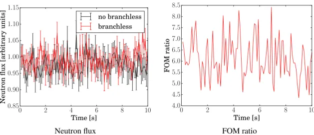
2.6 Branchless collisions . . . 54

2.6.1 Description of the algorithm . . . 54

2.6.2 Evaluating the efficiency of the method . . . 54

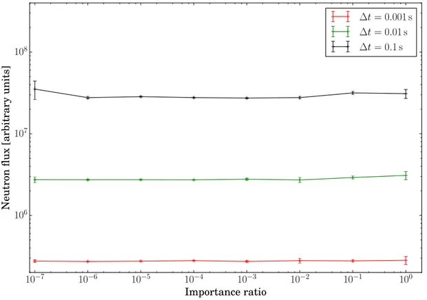
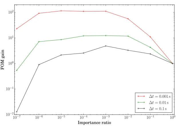
2.7 Development of a population importance method for fast kinetic configurations 56 2.7.1 Description of the algorithm . . . 56

2.7.2 Evaluating the efficiency of the method . . . 58

2.7.3 Choice of the optimal importance ratio . . . 58

2.8 Development of the capability to handle time-dependent geometry . . . 61

2.9 Conclusion . . . 62

3 Extensive tests of the kinetic methods 63 3.1 Verification tests on SPERT III E-core . . . 63

3.1.1 Presentation of SPERT III E-core . . . 63

3.1.2 Preliminary criticality calculations . . . 64

3.1.3 Steady state . . . 64

3.1.4 Reactivity insertion . . . 67

3.1.5 The role of precursors . . . 68

3.1.6 Rod drop . . . 69

3.2 Verification tests on the TMI 3x3 mini-core . . . 72

3.2.1 The TMI 3x3 mini-core . . . 72

3.2.2 Preliminary criticality calculations . . . 73

3.2.3 Reactivity insertions . . . 73

3.3 Investigating the correlations between time steps . . . 80

3.3.1 Critical configuration . . . 80

3.3.2 Subcritical configuration . . . 81

3.3.3 Fission chains length and impact on correlations . . . 81

3.3.4 Conclusion . . . 82

3.4 Investigating the impact of the scoring mesh spatial discretization . . . 83

3.4.1 Difference between kinetic and criticality calculations . . . 83

3.4.2 Dependence on the time step . . . 84

3.5 Conclusion . . . 86

II Dynamic Monte Carlo: time-dependent Monte Carlo neutron transport coupled with thermal-hydraulics 87 4 Development of a coupling between TRIPOLI-4 and thermal-hydraulics 88 4.1 Development of a multi-physics interface for TRIPOLI-4 . . . 88

4.1.1 Development of a supervisor . . . 88

4.1.2 Exchanging data from the mesh to the geometry . . . 89

4.1.3 Coupling between TRIPOLI-4 and SUBCHANFLOW . . . 90

4.1.4 Presentation of SALOME tools . . . 91

4.2 Criticality calculations with feedback . . . 92

4.2.1 Description . . . 92

4.2.2 Storing source capability . . . 95

4.3 Transient calculations . . . 95

4.3.1 Description . . . 95

4.3.2 Normalization between criticality and transient calculations . . . 96

4.4 Parallel calculations . . . 97

4.4.1 Thermal-hydraulics “rendez-vous” point . . . 97

4.4.2 Role of the different parallel units . . . 97

4.4.3 Memory footprint . . . 99

4.5 Conclusion . . . 99

5 Verification of the coupling for criticality simulations with feedback 100 5.1 Introduction on the benchmark work . . . 100

5.2 Description of the models used by the different codes . . . 100

5.2.1 TRIPOLI-4 and Serpent 2 models . . . 100

5.2.2 SUBCHANFLOW model . . . 101

5.3 Comparison between TRIPOLI-4 and Serpent 2 without feedback . . . 102

5.4 Description of the coupling schemes . . . 103

5.4.1 Architecture . . . 103

5.4.2 Convergence criteria . . . 103

5.5 Benchmark results with feedback . . . 104

5.5.1 Convergence . . . 104

5.5.2 Coolant temperatures and densities . . . 104

5.5.3 Fuel temperatures . . . 104

5.5.4 Comparison between calculations with and without feedback . . . 107

5.6 Conclusion . . . 110

6 Testing the coupling with dynamic simulations 111 6.1 Preliminary criticality calculations with feedback . . . 111

6.1.1 Critical boron search . . . 111

6.1.2 Source for the dynamic calculations . . . 111

6.2 Steady state . . . 115

6.3 Transients . . . 116

6.3.1 Control-rod extraction . . . 120

6.3.2 Control-rod extraction and reinsertion . . . 128

6.4 Conclusion . . . 132

III Preliminary analysis of the coupled system stability 133 7 Description of a simple model representative of the coupled system 134 7.1 Description of the problem . . . 134

7.2 The reference model . . . 134

7.2.1 Presentation of the deterministic coupled system . . . 134

7.3 From a deterministic to a stochastic system . . . 136

7.3.1 Adding Brownian noise . . . 136

7.3.2 Reparametrization . . . 137

7.3.3 Limitations of the modeling choices . . . 138

7.4 Preliminary results on Zt . . . 138

7.4.1 Linear equation . . . 138

7.4.2 Commutation of Atand As . . . 139

7.4.3 Alternative representation . . . 140

8 Analytical and numerical analysis of the model 141

8.1 Analysis of the Brownian term . . . 141

8.1.1 Gaussian process . . . 141

8.1.2 Properties of the matrix A . . . 141

8.1.3 Analysis of the covariance matrix . . . 142

8.1.4 Numerical simulations of the sytem . . . 145

8.1.5 Numerical simulations with TRIPOLI-4 . . . 146

8.1.6 Conclusion . . . 148

8.2 Analysis of the thermal-hydraulics coupling term . . . 149

8.2.1 Preliminary analysis . . . 149

8.2.2 Numerical simulations of the full system . . . 150

8.3 Simplified model . . . 153

8.3.1 Hypothesis . . . 153

8.3.2 Verification of the hypothesis . . . 153

8.3.3 Discussion on the non linearity . . . 153

8.4 Conclusion . . . 155 8.4.1 Brownian term . . . 155 8.4.2 Full system . . . 155 8.4.3 Discussion . . . 155 Conclusions 156 Appendix 162 A.1 Useful formulas for the point kinetics . . . 163

A.2 Flattop-Pu . . . 165

A.3 SPERT III E-core . . . 166

A.4 The TMI-1 3x3 mini-core . . . 168

A.5 Mathematical tools . . . 170

A.5.1 Itˆo process . . . 170

A.5.2 Useful properties on matrices . . . 170

A.5.3 Nomenclature for the analysis of the March-Leuba system . . . 171

A.5.4 Properties on the matrix A . . . 172

A.5.5 Correlation among time intervals . . . 173

A.6 Extended analysis of the TMI-1 3x3 mini-core dynamic simulations . . . 174

A.6.1 Time evolution of the fuel temperature . . . 174

A.6.2 Comparison between T4/SCF and SSS2/SCF . . . 174

R´esum´e en franc¸ais 177

The energy produced in nuclear reactors is released by interactions between neutrons and heavy nuclei contained in the fuel. One of the main issues for the study of a reactor behaviour is to model the propagation of the neutrons, described by the Boltzmann transport equation, in the presence of multi-physics phenomena, such as the coupling between neutron transport, thermal-hydraulics and thermomecanics. Pressurized water reactors (PWRs) are designed so as to ensure that the different feedback effects involved are negative: the feedbacks in the fuel and the mod-erator for example induce a decrease of the neutron flux in case of an initial increase in the reactivity of the neutron population. Operators are bound to prove safety authorities that any operation does not jeopardize the safety and stability of the reactor. For this purpose, design and safety analysis of nuclear reactors are performed with multi-physics simulation tools. Mod-eling the multi-physics behaviour is in fact highly challenging because of the vast number of unknowns, as well as the large size of the system, which implies simultaneously taking into ac-count nuclear interactions as well as macroscopic fluid motions and mechanical deformations. Most often, simulation tools for multi-physics are built by coupling separate simulation tools for each subfield of physics. This has the advantages of separating the concerns of the development of the different simulation tools and making the simulation more modular.

Concerning the Boltzmann neutron transport equation, two types of strategies are commonly applied. Deterministic methods numerically solve the equation by discretizing the phase space, at the expense of introducing approximations. Stochastic methods, called “Monte Carlo” meth-ods, are based on the random sampling of a large number of neutron trajectories. A mean value and an associated statistical uncertainty are determined for each observable of interest by tak-ing the ensemble averages over the simulated histories. Monte Carlo methods allow for an exact resolution of the transport equation, at the expense of a slow convergence of the statistical uncer-tainty on the results, which goes as 1/√N, N being the number of histories. In order to reduce the uncertainty, the most natural solution is to increase the statistics, i.e., the number of simu-lated trajectories. However, the slow convergence rate makes Monte Carlo a time-consuming method, even if it is well-suited for parallel calculations by nature. The computation time and memory footprint necessary for simulating real-size systems are very large and represent a seri-ous limitation of stochastic methods.

Because of these considerations, Monte Carlo methods are today almost exclusively devoted to criticality and fixed-source calculations, where the system is supposed to be at equilibrium (so that there is no time dependence) and thermal-hydraulics and thermomechanics quantities are supposed to be constant throughout the whole simulation. For such stationary calculations, Monte Carlo methods serve as reference tools for the verification of deterministic methods. Non-stationary scenarios such as transient accidents have been handled by deterministic codes only (Downar et al., 2002; Dulla et al., 2008; D’Auria et al., 2008; Gomez-Torres et al., 2012; Laureau et al., 2015; Knebel et al., 2016), until recent years. In order to extend Monte Carlo methods to non-stationary configurations so as to provide reference results for deterministic

tools for time-dependent problems, two paths must be explored. First, the so-called “kinetic” Monte Carlo shall explicitly take into account the time dependence in neutron transport, in-cluding the delayed neutrons. Second, the so-called “dynamic” Monte Carlo shall combine the kinetic methods with the physical feedbacks, such as thermal-hydraulics and thermomechanics.

Thermal-hydraulics concerns hydraulic flows in thermal fluids. This problem is described by non-linear equations, and there are different approaches to its solution. In nuclear reactors, it is customary to consider simplified versions of the problem by introducing different “scales” in relation to the size of the system under analysis: a global scale with system codes, a com-ponent scale with sub-channel codes or a local scale with computational fluid dynamics (CFD) codes. CFD codes solve fluid flow problems through turbulence models. They finely model the physical exchanges, at the expense of strong requirements of computation time and memory. This contrasts with sub-channel codes, which solve the equations on a coarser mesh, and pro-vide reliable (although approximate) and fast-running tools for the prediction of fluid flows in steady-state and transient configurations.

The development of reliable and fast numerical tools for the multi-physics simulation of reactor cores (coupling of neutron flux with thermal-hydraulics and thermomechanical feed-backs, in stationary and non-stationary regimes) has undergone intensive research efforts in re-cent years. This is witnessed by the innovation agendas SNETP, NUGENIA and H2020, and in particular the European projects NURESIM (2005-2008), NURISP (2009-2012), NURESAFE (2013-2015), HPMC (2011-2014) and McSAFE (2017-2020)1_{. Similar initiatives have been}

undertaken in China and in the USA (for instance, the CESAR2 _{project or the CASL}3

consor-tium). The final goal of these efforts is to pave the way towards a full “digital reactor core”, allowing even extreme (i.e., inaccessible to experimental evidence) conditions to be probed and the associated uncertainties to be quantified.

In order to understand the context of the work done in this field, in the following we provide a non-exhaustive list of the coupling efforts that have been conducted between Monte Carlo neutron transport and thermal-hydraulics codes, as well as of the development of kinetic Monte Carlo methods.

One of the first attempts at coupling a Monte Carlo and a thermal-hydraulics code appears to have been performed with the Monte Carlo code MCNP (X-5 Monte Carlo Team, 2003). Sev-eral couplings were set up, all in stationary conditions, i.e., without taking into account the time-dependence, and with thermal-hydraulics at different scales. The first used CFD codes, with the very first attempt (Mori et al., 2003) between MCNP4C (Briesmeister, 2000) and SIMMER-III (Yamano et al., 2003). However, because of the computation time limitation, only a one-set coupling was implemented: SIMMER-III was run as a first step, and the resulting temperatures and densities were introduced in the MCNP4C model, without any other thermal-hydraulics up-date. The first real couplings were later performed (Seker et al., 2007; Cardoni, 2011) between MCNP5 and the CFD codes STAR-CD (CD-adapco, 2005) and STAR-CCM+ (CD-adapco, 2009). Test cases were limited to small systems: up to a 3x3 array of pin cells.

Sub-channel codes have been also considered: an internal coupling between MCNP5 and the thermal-hydraulics sub-channel code COBRA-TF (Avramova and Salko, 2016) was

imple-1_{cordis.europa.eu/projects} 2_{cesar.mcs.anl.gov} 3_www.casl.gov

mented by Sanchez and Al-Hamry (2009). This enabled for stationary coupled calculations for a fuel assembly. In order to further increase the size of the simulated systems, MCNP5 was then coupled to the thermal-hydraulics system code ATHLET (Lerchl and Austregesilo, 1998) at as-sembly level (Bernnat et al., 2012). The speed of the system code made it possible to perform stationary coupled calculations on a full PWR core, in the context of the PURDUE bench-mark (Kozlowski and Downar, 2007). On-the-fly Doppler broadening was later introduced in MCNP to take into account the temperature dependence of the cross sections (Yesilyurt et al., 2012).

Intensive efforts were also made for multi-physics calculations with the Monte Carlo code Serpent 2 (Lepp¨anen et al., 2015). A multi-physics interface was implemented (Lepp¨anen et al., 2012), including internal solvers for the resolution of the heat transfer equation in the fuel and of hydraulics in the moderator. Serpent 2 can be also coupled with an external thermal-hydraulics solver. The temperature dependence of the cross sections was taken into account with the target motion sampling method (TMS) (Viitanen and Lepp¨anen, 2012, 2014).

Serpent 2 was internally coupled to the sub-channel code SUBCHANFLOW (Imke and Sanchez, 2012), using the multi-physics interface (Daeubler et al., 2015). This coupling was verified by code-to-code comparison on two 3x3 mini cores: against the coupling between the Monte Carlo code TRIPOLI-4® _{(Brun et al., 2015) and SUBCHANFLOW (Sjenitzer et al.,}

2015), and against the coupling between MCNP5 and SUBCHANFLOW (Ivanov et al., 2013a). The coupling work between Serpent 2 and SUBCHANFLOW also made it possible to perform coupled calculations on the full PWR benchmark mentioned above (Kozlowski and Downar, 2007). All the simulations concerned the stationary state of the reactor.

An external coupling between Serpent 2 and the thermal-hydraulics CFD code OpenFOAM (Open-FOAM Foundation, 2017) was then implemented through the multi-physics interface by Tuomi-nen et al. (2016) using external files. This work provided a new coupling between a Monte Carlo code and thermal-hydraulics at the CFD scale. Stationary calculations were performed on a fuel assembly with 4x4 pins (for this reduced test case, about 2 millions cells were used). However, extending these calculations to larger systems using this coupled tool seems hardly feasible, given the large number of cells required by CFD. Other couplings were recently performed with CFD codes, over small systems such as a pin cell (Wang et al., 2018), and even a TRIGA reac-tor (Henry et al., 2017).

All these works concerned stationary coupled calculations: up to full cores with sub-channel or system codes, or small systems with CFD codes. For the resolution of transient problems, the coupling infrastructure and the methods need to be adapted. For this purpose, the first step was the investigation of kinetic Monte Carlo methods: a summary of recent developments is given in the following.

Sjenitzer and Hoogenboom (2013) and Hoogenboom and Sjenitzer (2014) were the first to probe kinetic methods in a Monte Carlo code, for both TRIPOLI-4 and MCNP5, by tak-ing into account the precursors, and ustak-ing critical source sampltak-ing. Specific variance-reduction techniques for kinetic Monte Carlo were tested, such as forced precursor decay (L´egr´ady and Hoogenboom, 2008) and branchless collisions. Russian roulette and splitting and combing (Booth, 1996) were also implemented as population control techniques. Their work enabled the first Monte Carlo kinetic calculations for production neutron transport codes. Due to the high com-puter cost, kinetic simulations have been performed so far at the scale of fuel assemblies.

Kinetic methods were also implemented in the Monte Carlo code Serpent 2 by Lepp¨anen (2013). As a first step, delayed neutron emission was neglected and only prompt neutrons were considered. The new methods were verified by comparison to MCNP5 calculations on two small systems: Flattop-Pu and STACY-30 benchmarks (OECD Nuclear Energy Agency, 1995). This work was later extended to the treatment of delayed neutrons by Valtavirta et al. (2016).

Mylonakis et al. (2017) developed a transient module with kinetic methods for the Monte Carlo code OpenMC, including the generation of the critical source and the handling of one precursor group. The Russian roulette was also implemented as a population control method. The development of these methods made it possible to perform kinetic simulations of simplified systems.

In order to perform low computational cost kinetic calculations, (Laureau et al., 2015, 2017) has set up a time-dependent version of the fission matrix method. The matrices are computed once with a preliminary Monte Carlo criticality calculation, and are discretized in time. Then, the time evolution of the system is solved using the matrices.

GUARDYAN, a new Monte Carlo code for time-dependent calculations, was recently de-veloped (Molnar et al., 2019), using Graphics Processing Units (GPUs) for accelerated calcu-lations. Kinetic simulations of a whole core transient were performed on the Training Reactor at Budapest University of Technology and Economics, and validated against experimental data. A good agreement was obtained between simulation results and experimental data, showing an attractive application of GPUs for Monte Carlo simulations.

Finally, Sjenitzer et al. (2015) were the first to combine the kinetic methods with thermal-hydraulics. An external coupling was performed between TRIPOLI-4 and the sub-channel code SUBCHANFLOW. This work resulted in the first coupling between a Monte Carlo code and a thermal-hydraulics code in non-stationary conditions. Transient calculations were per-formed on a mini-core with 3x3 assemblies, and were compared to the results obtained by DYNSUB (Gomez-Torres et al., 2012), the coupling scheme between the deterministic code DYN3D (Grundmann et al., 2005) and the thermal-hydraulics sub-channel code FLICA (Toumi et al., 2000).

All these investigations reveal that, thanks to the growing computer power, it is now feasible to apply Monte Carlo methods to the calculation of non-stationary configurations. However, much progress must still be achieved for the kinetic Monte Carlo methods, which require spe-cific variance-reduction techniques in order to reduce the computational time. Moreover, kinetic methods and the coupling with thermal-hydraulics are most often handled separately. Also, the feedbacks are mostly dealt with by using sub-channel codes. In order to improve the accuracy of thermal-hydraulics modeling, attempts at coupling Monte Carlo neutron transport with CFD codes have been considered; however, further investigations are necessary in order to meet the different challenges listed above: computer time and memory handling.

The work performed in the present Ph. D. thesis provides some advances in the context of the coupled simulations of non-stationary neutron transport with thermal-hydraulics feedbacks. In particular, the goal of this Ph. D. thesis is to develop, verify and test a non-stationary coupling scheme between the Monte Carlo code TRIPOLI-4 and the thermal-hydraulics sub-channel code SUBCHANFLOW, so as to provide a reference tool for the simulation of reactivity-induced

transients in PWRs. The coupling is intended to be generic in scope, in order to simplify future couplings with thermomechanics and thermal-hydraulics codes via integration in the SALOME platform (Bergeaud and Lefebvre, 2010; SALOME, 2019). The stability and the robustness of the proposed algorithms are extensively analysed.

Plan of the thesis

This work is divided in three parts: first, the development of kinetic methods in TRIPOLI-4 is investigated, i.e., solving the time dependent neutron-precursor coupled problem without thermal-hydraulics feedbacks, with special focus on variance-reduction techniques for the time variable. Second, “dynamic” methods are adressed with the combination of kinetic methods with thermal-hydraulics via the development of a coupling scheme between TRIPOLI-4 and SUBCHANFLOW and the investigation of the resulting algorithms. Finally, a preliminary work for the stability analysis of the coupling scheme is presented. The detailed plan of the thesis is the following.

The physical mechanisms involved in a nuclear reactor are briefly recalled in Chapter 1. The basis of nuclear interactions is presented, as well as the two different approaches to solve the neutron transport equation: deterministic and Monte Carlo methods. The intimate coupling be-tween neutron transport, thermal-hydraulics and thermomechanics in PWRs is also introduced.

In Chapter 2, we illustrate the necessary methodology for kinetic simulations in TRIPOLI-4, without taking into account thermal-hydraulics feedbacks. The required algorithms are de-scribed, such as the time dependence, the sampling of the source, but also the population-control and variance-reduction techniques, which are necessary for kinetic calculations. A critique of the proposed methods is presented, which is essential to select the most suitable algorithms based on the characteristics of the system. We will focus in particular on the development of a new variance-reduction method carried out during the thesis. This new algorithm is well suited to fast kinetic configurations, where other methods fail to improve the statistics. The description of the method was published in Faucher et al. (2018), and its efficiency was assessed in Faucher et al. (2019a). Another key contribution is also presented: the capacity of TRIPOLI-4 to handle different input geometries within the same simulation, which is essential in order to update the system configuration during the time evolution, such as for the insertion or extraction of the control rods.

In Chapter 3, we will then verify the capacity of TRIPOLI-4 to perform kinetic simulations on realistic systems. Several simulations will be performed on the experimental reactor SPERT III E-core in different configurations: critical, control rod extraction and rod drop. The calcu-lations have been published in (Faucher et al., 2018) mentioned above. Other calcucalcu-lations are presented, on a mini-core based on the TMI-1 (Three Mile Island) reactor, and were published in a verification work through a comparison with the Monte Carlo code Serpent 2 for different reactivity insertions (?). We will also present our preliminary investigation of the correlations between time steps. The dependency of the relative uncertainty on the discretization of the ki-netic scoring mesh will be also examined.

The following step is to develop the coupling scheme between TRIPOLI-4 and SUBCHAN-FLOW: materials and methods are provided in Chapter 4. For this purpose, we have set up a multi-physics interface for TRIPOLI-4 through the development of an application program-ming interface (API) combined with an external supervisor that is able to control the TRIPOLI-4 simulation. Then, in order to couple TRIPOLI-4 and SUBCHANFLOW, we adhered to the spec-ifications of the SALOME platform, such as the ICoCo API for the coupling interface and the MEDCoupling library for the data exchange between the two codes. The architecture of the coupling scheme was published in Faucher et al. (2019b).

perform criticality calculations with thermal-hydraulics feedbacks, so as to provide the initial steady-state for coupled transients. As a verification test, we will perform a coupled calculation of an assembly based on the TMI-1 reactor, and we perform a code-to-code comparison with respect to the coupling scheme between Serpent 2 and SUBCHANFLOW. This work was de-scribed in the publication (Faucher et al., 2019b) mentioned above.

Then, in Chapter 6, we demonstrate the coupling scheme capability to simulate transients with thermal-hydraulics feedbacks. Calculations will be performed on the mini-core benchmark based on the TMI-1 reactor: first the system will be simulated at steady state so as to verify its stability; then we will introduce reactivity in the system so as to probe the effects of the thermal-hydraulics feedbacks.

Due to the stochastic nature of the outputs produced by TRIPOLI-4, uncertainties are in-herent to our coupling scheme and propagate along the coupling iterations. Moreover, thermal-hydraulics equations are non linear, so the prediction of the propagation of the uncertainties is not straightforward. The stability analysis of the coupling scheme is investigated in Chapters 7 (description of a simplified model) and 8 (analysis of the simplified model), in order to assess its convergence. This is a preliminary study aimed at quantifying the uncertainties in dynamic calculations.

List of published material

• Faucher, M., Mancusi, D., Zoia, A., 2018. New kinetic simulation capabilities for TRIPOLI-4®_{: Methods and applications. Ann. Nucl. Energy 120, 74 - 88.}

• Faucher, M., Mancusi, D., Zoia, A., Ferraro, D., Garcia, M., Imke, U., Lepp¨anen, J., Valtavirta, V., 2019b. Proceedings of the ICAPP 2019 conference. Juan-les-Pins, France. • Faucher, M., Mancusi, D., Zoia, A., 2019a. Proceedings of the M&C 2019 conference.

Portland, Oregon, USA.

• Ferraro, D., Faucher, M., Mancusi, D., Zoia, A., Valtavirta, V., Lepp¨anen, J., Sanchez Espinoza, V., 2019. Proceedings of the M&C 2019 conference. Portland, Oregon, USA. • Faucher, M., Mancusi, D., Zoia, A., 2020. Proceedings of the PHYSOR 2020 conference.

Description of the physical

mechanisms in a nuclear reactor

In this chapter we recall the key features of neutron transport with special emphasis on the time-dependent aspects, which are a key issue for understanding the different challenges encountered in this work. We also detail how nuclear reactor physics, thermal-hydraulics and thermome-chanics are intimately coupled.

1.1 Nuclear interaction probability

Neutron transport is characterized by the different types of nuclear interactions that can take place between an incident neutron and a target nucleus: for example, scattering, capture, or fission (Bell and Glasstone, 1970). All nuclear interactions are described by microscopic cross sections, which carry the dimensions of an area, usually expressed in units of barns (1 barn= 10−24_cm2_{). This value is roughly proportional to the cross-sectional area of the nucleus (the}

typical radius of a nucleus is about 10−12_{cm) and corresponds to the apparent area of the target}

particle as seen by the incident particle. Partial cross sections are also related to the probability of occurence of a given interaction: the higher the cross section for a given reaction type, the more likely is the interaction to occur.

Cross sections depend on the nature of the interaction but also on the nature of the incident and target particles, as well as on their energies. Cross sections can be experimentally measured at particular energies. Experimental data, often completed with the help of models, are evalu-ated and compiled into nuclear data libraries in standard format that can be read by transport codes. Examples of nuclear data librairies are JEFF-3.1 (Santamarina et al., 2009) or ENDF/B-VII (Chadwick et al., 2006).

At each collision, the probability of interaction is determined based on the partial cross sec-tion for each type of reacsec-tion, evaluated at the energy of the incident particle. For example, when an incident neutron collides with a heavy fissile nucleus, the fission probability is char-acterized by the ratio between the fission and the total cross sections. Figure 1.1 shows the microscopic fission cross section for uranium-235 (blue line), plotted against the energy of the incident neutron, for a range between 10−5_{eV and 30 MeV. The dependency on the neutron}

energy is clearly visible: the fission cross section is much larger at low (thermal) energies. The cross section for uranium-238 is also plotted (orange line): it is smaller than for uranium-235. In PWRs, water is used as moderator, and thermalizes neutrons through multiple collisions. In

10−5₁₀−4₁₀−3₁₀−2₁₀−1₁₀0 ₁₀1 ₁₀2 ₁₀3 ₁₀4 ₁₀5 ₁₀6 ₁₀7 Energy [eV] 10−10 10−8 10−6 10−4 10−2 100 102 104 F ission cross section [barn] uranium-235 uranium-238

Figure 1.1 – Fission cross section for uranium-235 (blue line) and uranium-238 (orange line), as a function of the energy of the incident neutron. Data come from the JEFF-3.3 library (table MT=18).

order to increase the probability of thermal fissions in PWRs, isotopes with high thermal fission cross sections must be used: this is why natural uranium, mainly consisting of uranium-238, is enriched in uranium-235.

1.1.2 Macroscopic cross sections

Macroscopic cross sections Σ are related to microscopic cross sections σ through the target particle density N [cm−3_]:

Σ = Nσ, (1.1.1)

and are expressed in cm−1_{. Macroscopic cross sections describe the probability for a neutron}

to interact with a material per unit length. For a material with k nuclei, the macroscopic cross section is given by

Σ = N1σ1+ N2σ2+ ... + Nkσk. (1.1.2)

1.2 Equations for neutron and precursor evolution

1.2.1 Transport equation for neutrons coupled with equation for precursors The angular neutron flux ϕ(r, 3, t) fully characterizes the system behaviour. It is defined by

ϕ(r, 3, t) = 3n(r, 3, t), (1.2.1)

withr the position vector, 3 the velocity, t the time, 3 = 3 · Ω the neutron speed, Ω the angular direction vector and n the neutron density.

The evolution of the neutron flux is described by the time-dependent Boltzmann equation, coupled with the equations for the precursors concentrations ci, j (with i the isotope and j its

precursor family), which read (Bell and Glasstone, 1970) 1 3 ∂ ∂tϕ(r, 3, t) + L ϕ(r, 3, t) = Fpϕ(r, 3, t) + X i, j χi, j_d (r, 3)λi, jci, j(r, t) + S(r, 3, t) (1.2.2)

and ∂ ∂tci, j(r, t) = Z νi, j_d (30_)Σi f(r, 3 0_{)ϕ(r, 3}0_{, t) d3}0 −λi, jci, j(r, t), (1.2.3)

with the net disappearance operator

L f = Ω · ∇ f + Σt(r, 3) f −

Z

Σs(r, 30 → 3) f (r, 30) d30, (1.2.4)

and the prompt fission operator

Fp f = X i χi p(r, 3) Z νi p(3 0_)Σi f(r, 3 0_{) f (r, 3}0_{) d3}0_{. (1.2.5)}

Notation is as follows:Σtis the total macroscopic cross section,Σsis the differential scattering

macroscopic cross section, χi

pis the normalized spectrum for prompt fission neutrons of isotope

i, νi

pis the average number of prompt fission neutrons of isotope i,Σf is the fission cross section,

χi, j_d is the normalized spectrum of delayed neutrons emitted from precursor family j of isotope i, λi, jis the decay constant of precursor family j of isotope i, νi, j_d is the average number of delayed

fission neutrons of precursor family j of isotope i, and the double sum is extended over all fissile isotopes i and over all precursor families j for each fissile isotope.

The equations above are completed by assigning the proper initial and boundary conditions for ϕ and ci, j. The quantity S(r, 3, t) represents the contribution due to an external source. We

have assumed here that all physical parameters (such as cross sections, velocity spectra, and so on) are time-independent (Keepin, 1965; Akcasu et al., 1971). If N fissile isotopes are present, each associated to M precursors families, Eqs. (1.2.2) and (1.2.3) form a system of 1+ N × M equations to be solved simultaneously. In order to keep notation simple in the following, we will only consider one isotope, so we drop the index i on the isotopes.

1.2.2 Eigenmode decomposition k-eigenmodes

We consider the system without external source, i.e. S(r, 3, t) = 0. By replacing the precursor Eq. (1.2.3) into Eq. (1.2.2) for the neutron flux, we get

1 3 ∂ ∂tϕ(r, 3, t) + L ϕ(r, 3, t) = Fpϕ(r, 3, t) + X j χj d(r, 3) Z νj d(3 0_)Σ f(r, 30)ϕ(r, 30, t) d30 −X j χj d(r, 3) ∂ ∂tcj(r, t). (1.2.6)

Now if we seek a stationary solution of Eq. (1.2.6), we get

L ϕ(r, 3) = Fpϕ(r, 3) + X j χj d(r, 3) Z νj d(3 0_)Σ f(r, 30)ϕ(r, 30) d30. (1.2.7)

By defining the total fission operator F = Fp+ Fd, including the prompt fission operator, as

defined by Eq. (1.2.5), and the delayed fission operator

Fd f = X j χj d(r, 3) Z νj d(3 0_)Σ f(r, 30) f (r, 30) d30, (1.2.8)

Eq. (1.2.7) can be rewritten as

L ϕ(r, 3) = F ϕ. (1.2.9)

The k-eigenmodes ϕkassociated to the Boltzmann equation Eq. (1.2.2) emerge by imposing that

the system should be exactly critical without external sources and asking by which factor k the fission terms should be rescaled in order to make the time derivative vanish (Bell and Glasstone, 1970; Cullen et al., 2003):

L ϕk(r, 3) = 1

k F ϕk(r, 3). (1.2.10)

α-eigenmodes

For bounded domains, using the separation of variables, an exponential relaxation of the kind

ϕ(r, 3, t) = ϕα(r, 3)eαt (1.2.11)

and

cj(r, t) = c j

α(r)eαt (1.2.12)

may be postulated for both the neutron flux and the precursors concentrations. Here the value α represents the relaxation frequency (Bell and Glasstone, 1970; Duderstadt and Martin, 1979). Eqs. (1.2.11) and (1.2.12) can be more rigorously justified by resorting to Laplace transform or equivalently to spectral analysis (Duderstadt and Martin, 1979). Yet, proving the feasibility of such a relaxation is highly non-trivial in general, and precise (although not very restrictive) conditions are required on the geometry of the domain and on the material cross sections (Bell and Glasstone, 1970; Larsen and Zweifel, 1974; Duderstadt and Martin, 1979). Here, for the sake of simplicity, we will assume that such conditions are met (which is typically the case for almost all systems of practical interest) and that separation of variables is allowed.

Then, substituting Eqs. (1.2.11) and (1.2.12) into Eqs. (1.2.2) and (1.2.3), respectively, yields the (coupled) natural eigenmode equations

α 3ϕα(r, 3) + L ϕα(r, 3) = Fpϕα(r, 3) + X j χj d(r, 3)λjc j α(r) (1.2.13) and αcj α(r) = Z νj d(3 0_)Σ f(r, 30)ϕα(r, 30) d30−λjcαj(r), (1.2.14)

which formally represent a system of eigenvalue equations for the flux ϕαand the precursors cαj,

the eigenvalues being α.

It is customary to formally solve Eq. (1.2.14) for the precursor concentration and to replace the resulting cj

α into Eq. (1.2.13). This yields the eigenvalue problem for ϕα(Weinberg, 1952;

Cohen, 1958; Henry, 1964; Bell and Glasstone, 1970) α 3ϕα(r, 3) + L ϕα(r, 3) = Fpϕα(r, 3) + X j λj λj+ α F_djϕα(r, 3). (1.2.15)

The inverse of the largest eigenvalue α0 for this equation is commonly referred to as the

“re-actor period” (Cohen, 1958; Henry, 1964; Kaper, 1967; Bell and Glasstone, 1970). It provides information on the asymptotic time behaviour of the system in any regime. For an example of application of the dominant natural eigenvalue in reactor physics, see, e.g., Zoia et al. (2014a, 2015).

Observe that, if α= 0 is an admissible dominant eigenvalue of Eq. (1.2.15), then Eq. (1.2.10) admits a solution with k = 1 and ϕα = ϕk. Contrary to the k-eigenmodes Eq. (1.2.10), the

natural eigenmode Eqs. (1.2.13) and (1.2.14) are well defined also for non-multiplying systems,

in which case we have _α

3ϕα(r, 3) + L ϕα(r, 3) = 0. (1.2.16) 1.2.3 Point-kinetics via the k-eigenmodes

The so-called point-kinetics equations are introduced in reactor physics so as to condense the behaviour of the neutron and precursor population to a model where only the time dependence is left (Bell and Glasstone, 1970). The equations are formally obtained from the exact time-dependent Boltzmann equation weighted by the adjoint flux. The equation adjoint to Eq. (1.2.10) is L†ϕ†_k(r, 3) = 1 k F †_ϕ† k(r, 3). (1.2.17) where ϕ†

k denotes the adjoint critical eigenmode for the neutron flux, and the adjoint of a linear

operator L is defined as customary via the relation

hL f, gi = h f, L†gi, (1.2.18)

with h f, gi the scalar product between functions f and g.

The first step consists in multiplying the time-dependent Eq. (1.2.2) by the fundamental adjoint k eigenmode and by multiplying the equation for the adjoint k eigenmode by the time-dependent neutron flux ϕ(r, 3, t). The resulting equations are then integrated over space, energy and angle, which yields

∂ ∂thϕ † k(r, 3), 1 3ϕ(r, 3, t)i + hϕ † k(r, 3), L ϕ(r, 3, t)i = hϕ† k(r, 3), Fpϕ(r, 3, t)i + X j λjhϕ†_k(r, 3), χ_dj(r, 3)cj(r, t)i (1.2.19) and hϕ(r, 3, t), L†_ϕ† k(r, 3)i = 1 khϕ(r, 3, t), F †_ϕ† k(r, 3)i. (1.2.20)

By subtracting these equations from each other and using Eq. (1.2.18), we get ∂ ∂thϕ † k, 1 3ϕi + 1 khϕ † k, F ϕi = hϕ † k, Fpϕi + X j λjhϕ†_k, χ_djcji, (1.2.21)

which we can rewrite as ∂ ∂thϕ † k, 1 3ϕi = k −1 k hϕ † k, F ϕi − hϕ † k, Fdϕi + X j λjhϕ†_k, χ_djcji. (1.2.22)

Now, suppose that the time-dependent neutron flux can be factorized as ϕ(r, 3, t) ' ˜n(t)ϕk(r, 3),

i.e., the product of the fundamental k eigenmode (acting as a position- and velocity-dependent shape factor) times an amplitude factor ˜n(t) that depends only on time. This approximation is assumed to be valid for small departures from the critical point, i.e., when k ' 1. By replac-ing this flux decomposition into Eq. (1.2.22) we obtain an equation for the neutron population amplitude ˜n(t), namely, ∂ ∂t˜n(t)= ρ − βeff Λeff ˜n(t)+ X j λj˜cj(t), (1.2.23)

where we have defined the so-called static reactivity

ρ = k −1

k , (1.2.24)

the effective delayed neutron fraction βeff = hϕ† k, Fdϕki hϕ† k, F ϕki , (1.2.25)

the effective mean generation time

Λeff = hϕ† k, 1 3ϕki hϕ† k, F ϕki , (1.2.26)

and the effective precursor concentrations ˜cj(t)= hϕ† k, χ j dcji hϕ† k, 1 3ϕki . (1.2.27)

The kinetics parameters βeff andΛeff appearing in Eq. (1.2.23) are called “effective” because

they have been weighted by the adjoint eigenmode, which physically represents the asymptotic importance of the neutron population in a multiplying system (Keepin, 1965; Bell and Glas-stone, 1970).

Eq. (1.2.23) yields the time evolution of the neutron population, under the approximations introduced above. The neutron evolution must be coupled to the equations for the effective precursor concentrations, which can be derived by following the same arguments as above, and read

∂ ∂t˜cj(t)=

βj,eff

Λeff ˜n(t) − λj˜cj(t), (1.2.28)

where we have defined the effective delayed neutron fractions pertaining to each family j, i.e., βj,eff= hϕ† k, F j dϕki hϕ† k, F ϕki . (1.2.29)

Other useful formulas for point-kinetics analysis are provided in Sec. A.1.

1.3 Fission chains

After a fission reaction with the incident neutron, the fissile nucleus typically splits in two lighter nuclei, called fission products. Other particles are also emitted, including new neutrons, which may trigger new fissions. This branching process, where neutrons give birth to other neutrons, is called a “fission chain”, the control of which is essential for the operation of a reactor. A fission chain ends when there are no more neutrons to induce new fissions, i.e., when all neutrons from the fission chain got captured or leaked out of the system.

1.3.1 Multiplication factor

To define the sustainability of a fission chain, the effective neutron multiplication factor keffis

de-fined as the average ratio between the number of neutrons in successive generations. When each fission causes one fission on average, the effective neutron multiplication factor keffis equal to

1 and the system is called “critical” (Keepin, 1965). In this case, the reaction is self-sustaining. Such stable chain is the basis for energy production in a nuclear reactor. If keffit larger than 1,

the system is “supercritical”; in the absence of feedback effects, there is an exponential growth of the neutron population. Conversely, if is is smaller than 1, the system is “subcritical” and the population eventually dies out.

Another quantity commonly used to characterize the sustainability of the fission chains is called the “reactivity”, which is defined as

ρ = keff−1

k_eff . (1.3.1)

It is usually measured in pcm (1 pcm= 10−5_{), or in dollars (1 $ = β}

eff, with βeff the effective

delayed neutron fraction defined by Eq. (1.2.25)). The reactivity expresses the deviation from the system with respect to criticality.

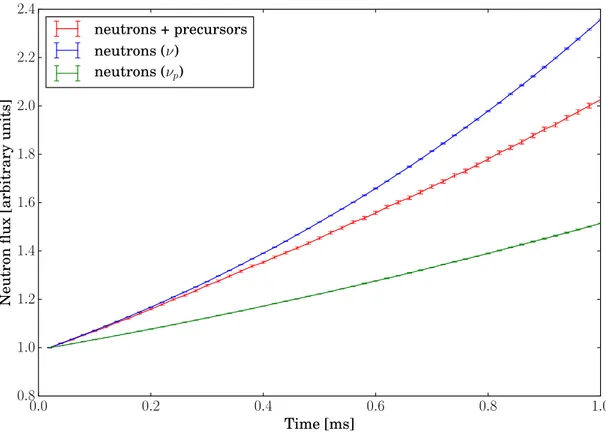
1.3.2 Neutrons and precursors

Two types of neutrons are released by fission, as illustrated in Fig. 1.2: prompt neutrons, emitted almost instantaneously after fission, and delayed neutrons, coming from the β−_{decay of}

unsta-ble fission products, called “precursors” (Keepin, 1965). Precursors are characterized by their decay constant λ [s−1], i.e., the average decay time for a fission product to give rise to a delayed neutron by β−_{decay. In nuclear data librairies, the different precursors are regrouped in families}

depending on their decay time (e.g., there are 8 families in the JEFF-3.1 library (Santamarina et al., 2009)).

Prompt and delayed neutrons have very different characteristics, as detailed below and sum-marized in Table 1.1. Here, λ is the typical decay constant of the precursors (each precursor family j has its own decay constant λj). All the parameters depend on the fuel composition and

the configuration of the reactor core.

The prompt multiplication factor kpand the delayed multiplication factor kdcan be defined

as

kp= (1 − βeff) × keff, (1.3.2)

kd= βeff× keff, (1.3.3)

k_eff= kp+ kd. (1.3.4)

Energy

Prompt neutrons are emitted with an average kinetic energy around 2 MeV. Yet, as mentioned in Sec. 1.1, fission is more likely to happen when the energy of the incident neutron falls below 1 eV. Because of their large emission energy, prompt neutrons have to slow down before in-ducing fission. In contrast, delayed neutrons are created with a lower energy (around 400 keV),

prompt neutrons delayed neutrons

emission energy 2 MeV 400 keV

associated time scale Λeff ≈ 20µs λ−1 ≈ 1 s average number per fission νp ≈ 2.4 νd ≈ 0.017

Table 1.1 – Different characteristics of prompt and delayed neutrons (typical values for uranium-235 are given, with βeff ≈700 pcm).

and therefore are less likely to disappear by leakage or capture, before inducing fission. Essen-tially, delayed neutrons have a higher probability to induce a thermal fission (Duderstadt and Hamilton, 1976).

The delay of delayed neutrons

Neutrons and precursors have very different typical time scales; the generation time for prompt neutrons is aboutΛeff ≈ 20µs, while the precursors decay time is about λ−1 ≈ 10 s (these are typical values for a PWR). Because of this difference of scale, delayed neutrons slow down the time evolution of the system due to a change in reactivity. This is the reason why delayed neu-trons play a major role in nuclear reactor control.

In a critical system (keff = 1), there are (1 − βeff) prompt neutrons and βeffdelayed neutrons.

Thus, the neutron effective lifetime leff, combining prompt and delayed neutrons lifetime, is

defined as (Duderstadt and Hamilton, 1976)

l_eff = (1 − β_eff) ×Λ_eff+X

j β_{eff, j}(_λ1 j + Λeff ) (1.3.5) = Λeff+ X j βeff, j λj . (1.3.6) Unbalanced ratio

The quantities βeff/Λeffand λ provide the rates at which a neutron is converted into a precursor,

and conversely. The typical ratio βeff/(λ × Λeff) is of the order of 104 for water-moderated

reactors. This implies that, when the neutron and precursor populations are in equilibrium, precursors are considerably more abundant than neutrons within the core. This suggests that the Monte Carlo simulation of such unbalanced populations (in terms of size and time scale) requires strategies and variance-reduction techniques that are distinct from those of stationary simulations.

1.3.3 Fission chain length

When kp < 1, prompt fission chains are finite and eventually die out. Criticality is ensured by

the presence of delayed neutrons. Indeed, each fission chain produces on average one precursor, which emits a delayed neutron after a decay time larger than the chain lifetime, thus after the prompt fission chain has died. Therefore, the delayed neutron does not participate in the fission chain that created it but starts a new one instead. In such cases (kp< 1), the average length ¯n of

neutron fissile nucleus precursor prompt neutrons fission product fission product delayed neutron Figure 1.2 – Schematic depicture of neutron-induced fission with the different particles pro-duced. After the fission, prompt neutrons and precursors are emitted almost instantaneously while delayed neutrons are emitted after precursors decay.

the fission chain is given by (Sjenitzer and Hoogenboom, 2011a): ¯n= _{1 − k}1

p

. (1.3.7)

For instance, if the system is exactly critical, kp= 1 − βeff, and the average fission chain length

is ¯n= 1/βeff.

When the system is prompt critical or supercritical (i.e., kp≥1), however, prompt neutrons

alone are sufficient to maintain the chains, and some chains grow indefinitely. Some neutrons might get prematurely captured or leak, thus terminating the chain, but on average the fission chains are infinite.

1.4 Deterministic methods for solving transport equation

Deterministic methods solve the Boltzmann transport equation by discretizing the phase space: space, energy, time and angle (for instance, SN for the decomposition on discrete directions, PN

for an expansion on the spherical harmonics and SPN, simplified PN). The advantage of such

methods is a reasonable computation time, obtained at the expense of discretization errors. Until very recently, the simulation of neutron transport in non-stationary conditions was entirely based on deterministic methods (which are usually fast for stationary conditions). For transient regimes, due to the very large number of unknowns (∼ 1014_{) resulting from a fine}

discretization of phase space variables (space, angle, velocity and time), current state-of-the-art industrial codes employ a two-step approach: a detailed transport calculation at the lattice scale in stationary conditions in two dimensions is followed by a time evolution calculation for the neutron flux at the core scale, based on the cross sections determined in the course of the first step. The time-dependent step is typically carried out in simplified transport models (diffusion or SPN, for instance) with a coarse energy discretization (Smith, 1979; D’Auria et al., 2004;

Since the approximations introduced in the deterministic approach are problem-dependent (i.e., specific to each reactor type), the validity of the results thus obtained, as well as the as-sessment of the associated uncertainties, depend on the configuration under analysis (D’Auria et al., 2004; Dulla et al., 2008; Larsen, 2011). Thus, in order to relax these constraints and to consolidate the validation of deterministic codes, it is mandatory to develop a best estimate method (IAEA, 2003). This is especially true in view of the small number of experimental measurements available for transient reactor operation or accidents (IAEA, 2015).

1.5 Monte Carlo particle transport

Monte Carlo simulation is based on the realization of a large number of stochastic neutron trajectories, whose probability laws are determined in agreement with the underlying physical properties (the probability of particle-matter interaction, energy and angle distributions after collision, and so on). The transport simulation follows a random walk from one interaction to the next. The distance to the next collision is sampled according to the total macroscopic cross section; the particle is transported to this point and finally the interaction is sampled depending on the nucleus at the collision site. Monte Carlo methods allow for an exact treatment of the re-actor geometry (Lux and Koblinger, 1991). Accordingly, Monte Carlo simulation is considered as the “golden standard” for neutron transport calculations (Bell and Glasstone, 1970; Lux and Koblinger, 1991).

Consider the time-independent version of Eq. (1.2.2) L ϕ(r, 3) = Fpϕ(r, 3) + X j χj d(r, 3)λjcj(r) + S(r, 3), (1.5.1) where cj(r) = 1 λj Z νj d(3 0_)Σi f(r, 3 0_{)ϕ(r, 3}0_{) d3}0_{. (1.5.2)}

This equation describes a so-called “fixed-source” problem; in the following we will show how the problem is adressed with a Monte Carlo simulation. A source and a detector must be defined in the phase space. The purpose of the simulation is to estimate the response in the detec-tor, meaning collecting the contributions of neutrons reaching a given phase-space region. In practice, N neutrons are emitted from the source and are transported through the phase space. Assuming that the simulated system is made of a homogeneous medium characterized by a total macroscopic cross sectionΣt, the exponentially distributed distance x between two interactions,

travelled by a neutron with an energy E, is sampled from the equation

x= − 1 Σt(E)

ln(1 − ξ), (1.5.3)

with ξ a random number, uniformly distributed in the interval [0,1]. Note that, if the space is not homogeneous, the flight has to be split in different volumes, and, if x is larger than the distance to the boundary of the particle initial volume, the particle is first stopped at the volume boundary and the next flight length is then sampled.

At the new sampled position, the interacting nucleus k is chosen with probability

pk = Σ k,t(E)

Σt(E)

withΣk,t(E) the total macroscopic cross section for nucleus k.

Finally, the interaction l on nucleus k is sampled using the probability

pk,l= σ_σk,l(E)

k,t(E), (1.5.5)

with σk,l(E) the microscopic cross section for nucleus k associated to the interaction l.

After the interaction, if the neutron is still alive (it can be absorbed, or killed by the Russian roulette presented in Sec. 1.5.2), the distance to the next collision is sampled, and so on, until the particle is killed or the simulation stops. Neutron contributions are collected if they reach the detector. The whole process of transporting N particles is repeated M times (i.e., the statistical ensemble) with a different random seed each time.

The contributions being averaged over M independent replicas, the result comes with a statistical uncertainty on the ensemble average, which is inversely proportional to square root of the number of histories. Thus, the only reason for fluctuations in the results is the limited number of simulated trajectories. In order to accumulate significant statistics, Monte Carlo codes must simulate a large amount of particles. The order of magnitude is problem-dependent but it is usually very large. Hence, Monte Carlo simulations are very time-consuming. Fortunately, Monte Carlo particle transport codes generally have excellent parallel scalability, and are even sometimes “embarrassingly” parallel (Rosenthal, 1999). Indeed, since neutron histories are independent, each processor can follow its own set of particles. Parallel simulation allows for a considerable speed-up, in principle of the order of the number of available processors. When all processors have completed the simulation of particle histories, the final results are collected.

1.5.2 Variance-reduction and population-control techniques

The convergence of Monte Carlo simulations directly depends on the number of simulated par-ticles, which also governs the computation time. In order to improve the convergence without slowing down the computation time, physical laws are not systematically enforced; it is possible to alter the physical processes as long as a compensation is applied elsewhere to keep the results unbiased. For this purpose, a so-called “statistical weight” is assigned to each particle at the be-ginning of the simulation, and evolves along the simulation so as to compensate the introduced changes in the sampling rules. However, the “variance-reduction” techniques require to control the statistical weights and size of the population in order to ensure that they do not vary too much. Such Monte Carlo simulations are called “non-analog”, as opposed to those preserving the regular sampling laws, which are called “analog”. The most representative examples of a variance-reduction technique, implicit capture, and of a population-control technique, Russian roulette and splitting, are presented below.

Implicit capture

In the absence of fission, a neutron having a collision can be either scattered or captured. In the second case, it is “killed”, meaning it is removed from the simulation. The probability pafor a

neutron having a collision to be absorbed is pa =

σa

σt

, (1.5.6)

and the complementary probability psnot to be absorbed (i.e., to be scattered) is

ps= 1 −

σa

σt

with σa the microscopic absorption cross section and σt the microscopic total cross section.

Implicit capture allows the particles to explore the phase space rather than being absorbed. In other words, particles are forced to scatter. In order to preserve a fair Monte Carlo game, the particle weights are multiplied by a factor ps < 1. This way, the neutron weight decreases at

each collision.

Russian roulette and splitting

At some point in the simulation, particle weights may become very low (for instance because of implicit capture). In that case, particles slow down the calculation without contributing much to the statistics. With implicit capture preventing particles to be absorbed, only leakage can kill particles. Thus, implicit capture has to be combined with other methods. The Russian roulette method helps to terminate particle histories. If the particle weight drops below a predefined threshold (usually 0.8), then a random number is generated. If it is below the initial weight, the particle is killed. Otherwise, its weight is set to a predefined value (usually 1). On the contrary, if the particle weight is above another predefined threshold (usually 2), it is split into several particles, each carrying a fraction of the original weight.

1.5.3 TRIPOLI-4

TRIPOLI-4 is a 3D continuous-energy Monte Carlo particle transport code devoted to shielding, reactor physics, criticality-safety and nuclear instrumentation. It can solve both fixed-source transport and eigenvalue problems. The code has been developed at CEA Saclay since the mid 90s in C++, with a few parts in C and Fortran. It uses nuclear data evaluation files written in ENDF format. For the temperature dependence of the cross sections, stochastic interpolation was implemented. TRIPOLI-4 supports execution in parallel mode. More details on this code can be found in Brun et al. (2015). The work presented in this thesis was performed within a development version of TRIPOLI-4.

1.6 Coupling between neutron transport, thermal-hydraulics and

thermomechanics

A nuclear reactor is a complex system whose behaviour depends on the strong coupling between neutron transport, thermal-hydraulics and thermomechanics. The feedback effects involved are essential to the reactor stability. Indeed, a PWR is designed so as to ensure that the feedback effects are negative: any increase or decrease in the neutron power causes thermal-hydraulics and thermomechanics feedbacks that counter-react these variations and thus keep the reactor power stable. The main feedback effects are listed below.

1.6.1 Description of the feedback effects

As discussed above, microscopic cross sections strongly depend on the energy of the incident neutron. As a consequence, microscopic cross sections are also temperature-dependent, because of thermal motion of the collided nuclei, mainly via the Doppler effect. Moreover, macroscopic cross sections depend on the temperature also via the density effect, which affects the concen-trations of the nuclei per unit volume.

Fuel temperature

When the fission power increases, the fuel temperature also increases, inducing modifications of cross sections. The most visible effect is the so-called “Doppler broadening” of the resonances in

the radiative capture cross section of uranium-238. The thermal motion of target nuclei changes the shape of the resonances: they become wider and flatter. With Doppler effect, neutrons are more likely to be captured on uranium-238 and less likely to induce fission on uranium-235, which leads to a decrease in fission power, thereby stabilizing the system. In a typical PWR, the Doppler coefficient αF T, is defined as αF T = 1 k_eff dk dTF , (1.6.1)

with TF the fuel temperature, and ranges from−1 pcm/K to −4 pcm/K (Duderstadt and

Hamil-ton, 1976).

Moderator temperature and density

When the moderator temperature increases, neutrons are less slowed down, and the neutron spectrum is hardened. This results in a reduction of absorption in uranium-235 as compared to absorption in uranium-238. Therefore, the power decreases.

The main moderator effect occurs from changes in the density. When the moderator density decreases, the macroscopic cross section decreases and the moderator becomes less efficient to slow down the neutrons. Therefore, neutrons are less efficient at inducing fission, the power decreases and the reactivity decreases. The two feedback effects in the moderator improve reactor stability. The moderator coefficient αM

T, is defined as αM T = 1 k_eff dk dTM , (1.6.2)

with TMthe moderator temperature, and ranges from−8 pcm/K to −50 pcm/K (Duderstadt and

Hamilton, 1976).

Thermomechanics

The heating in the reactor core induces thermal expansion and deformation of the different elements. For example, the fuel pellets expand at the expense of the gas gap, whose width decreases. As a result, the heat transfer between the fuel pellet and the cladding increases.

1.6.2 Thermal-hydraulics solvers

Fluid dynamics is described by non-linear conservation equations, and different approaches exist for their solution. For example, CFD codes finely model the physical exchanges, at the expense of strong requirements in terms of computation time and memory. Sub-channel codes are faster but make some approximations and solve the equations on a coarser mesh. Even if they provide approximate solutions, they are reliable tools and are often used to study thermal-hydraulics phenomena in nuclear reactor cores. System codes rely on an even less detailed description of the physics and provide the response of the components under consideration in the form of global averages. In the following, we focus on the sub-channel approach, which is used in this work.

A sub-channel is the flow area delimited by adjacent fuel rods. Sub-channel codes only consider two directions of the flow through sub-channels: axial and lateral (lateral covers all directions orthogonal to axial direction). The axial length of each sub-channel is divided in slices, and the flow is transmitted through these axial volumes. The axial flow is usually treated

as the dominant one-dimensional flow, and the lateral flow is simplified. Lateral flow is assumed to enter a channel volume through “gaps”, formed by adjacent fuel rods. Examples of sub-channel codes are COBRA-TF (Avramova and Salko, 2016), FLICA (Toumi et al., 2000) and SUBCHANFLOW (Imke and Sanchez, 2012).

1.6.3 Conservation equations

Fluid dynamics is based on three fundamental equations, which are conservation equations for mass ∂ρ ∂t +∇ ·(ρ − → V)= 0, (1.6.3) momentum ∂(ρ→−V) ∂t + ∇ · ( − → V ⊗ρ→−V) − ∇ · τ+ ∇P = ρ−→g, (1.6.4) and energy ∂ρ ∂t(ρ(e+ |→−V |2 2 ))+ ∇ · (ρ(e + − → V2 2 ) − → V) − ∇ · −→ϕ = ∇ · (τ ·→−V)+ ρ−→g ·→−V − ∇ ·(P→−V), (1.6.5) with ρ the density,→−V the field velocity, ⊗ the outer product, τ the stress vector, P the pressure, −

→_{g the gravity acceleration vector, e the internal energy and −}→_{ϕ the conductive heat flux vector.}

Because of the limitation of the flow to two directions for sub-channel solvers, approx-imations are introduced in the conservation equations. For instance, for mass conservation, Eq. (1.6.3) becomes ∂ρ ∂t + ∂(ρVx) ∂x + 1 Awk= 0, (1.6.6)

with Vxthe axial speed, A the sub-channel flow area and wkthe linear mass flow rate (kg m−1s−1)

through the k-th gap.

Then, mass, momentum and energy conservation equations are discretized over the cells of the mesh with a finite difference scheme. The resulting equations simultaneously solved by SUBCHANFLOW in each cell are presented below (Imke and Sanchez, 2012).

Mass conservation Ai, j∆X_∆tj(ρi, j−ρi, jold)+ (mi, j− mi, j−1)+ ∆Xj X k wk, j = 0. (1.6.7) Momentum conservation

The momentum conservation equation is decomposed in two equations: axial momentum ∆Xj ∆t (mi, j− moldi, j)+ mi, jU 0 i, j+ ∆Xj X k wk, jU_{k, j}0 = −Ai, j(pi, j− pi, j−1) − gAi, j∆Xjρi, j − 1 2( ∆X f φ2 Dhρl + Kv 0₎ i, j|mi, j|mi, j Ai, j −∆Xj X k w0_{k, j}(U_{i, j}0 − U_{n(k), j}0 ), (1.6.8)

and lateral momentum (where convective transport is neglected) ∆Xj ∆t (wk, j− woldk, j)+ ( ¯Uk, j0 wk, j− ¯Uk0, j−1wk, j−1)= sk lk∆X j∆pk, j−1−(KG ∆Xv0 k sklk )j|wk, j|wk, j. (1.6.9)

Energy conservation Ai, j ∆t[ρ 00 i, j(hi, j− holdi, j)+ hi, j(ρi, j−ρoldi, j)]+ _∆X1 j (mi, jhi, j− mi, j−1h_{i, j−1}) (1.6.10) +X k wk, jhk, j= Qi, j−X k w0_{k, j}(hi, j− hn(k), j). (1.6.11)

Notation in the previous expressions is as follows:

i: channel index, j: slice index, k: gap,

n(k) : channel neighbor belonging to gap k, A: cross-sectional area of the sub-channel, ∆X : axial cell length (m),

∆t : time step (s),

m: axial mass flow rate (kg s−1), h: specific mixture enthalpy (J K−1), hfg: evaporation enthalpy (J K−1),

Q: linear power released to the sub-channel (W m−1), w0 : turbulent cross-flow (kg m−1s−1),

p: pressure at axial boundary (Pa), f : single-phase friction coefficient, g: gravity (m/s2),

φ2_{: two-phase friction multiplier,}

Dh: hydraulic diameter (m),

K : axial pressure loss coefficient, KG: lateral gap pressure loss coefficient,

s: gap width between two neighboring rods (m), l: distance of neighboring sub-channels midpoints (m), ρ00 _{= ρ}old − hfg∂ψ_∂h, ψ = ρliqx(1 − α) − ρvap(1 − x), x: steam quality, α : void fraction, v0 = x 2 αρvap + (1 − x)2 (1 − α)ρliq, U0 = m Av 0_, liq : liquid, vap : vapor,